Grad-PU: Arbitrary-Scale Point Cloud Upsampling via Gradient Descent with Learned Distance Functions
Abstract
Most existing point cloud upsampling methods have roughly three steps: feature extraction, feature expansion and 3D coordinate prediction. However, they usually suffer from two critical issues: (1) fixed upsampling rate after one-time training, since the feature expansion unit is customized for each upsampling rate; (2) outliers or shrinkage artifact caused by the difficulty of precisely predicting 3D coordinates or residuals of upsampled points. To adress them, we propose a new framework for accurate point cloud upsampling that supports arbitrary upsampling rates. Our method first interpolates the low-res point cloud according to a given upsampling rate. And then refine the positions of the interpolated points with an iterative optimization process, guided by a trained model estimating the difference between the current point cloud and the high-res target. Extensive quantitative and qualitative results on benchmarks and downstream tasks demonstrate that our method achieves the state-of-the-art accuracy and efficiency.
†† Yun He and Xiangyang Xue are with the School of Computer Science, Fudan University.†† Yanwei Fu is with the School of Data Science, Fudan University. He is also with Shanghai Key Lab of Intelligent Information Processing, and Fudan ISTBI–ZJNU Algorithm Centre for Brain-inspired Intelligence, Zhejiang Normal University, Jinhua, China.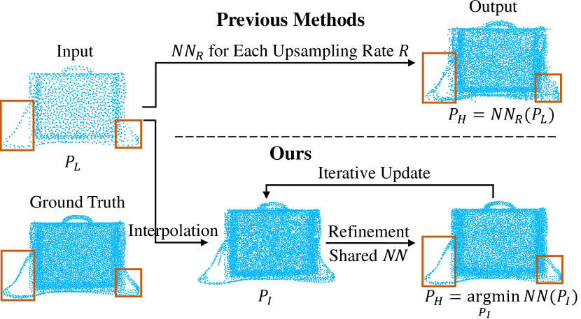
1 Introduction
With the popularity of commercial 3D scanners, capturing point clouds from real-world scenes becomes convenient and affordable. Thus point clouds have been widely utilized in applications such as autonomous driving, robotics, remote sensing, etc [11]. That being said, the raw point clouds produced by 3D scanners or depth cameras are often sparse and noisy, sometimes with small holes [17], which greatly affects the performance of downstream tasks, such as semantic classification [40], rendering [5], surface reconstruction [1], etc. Consequently, it is vital to upsample a raw point cloud to a dense, clean and complete one, with more geometric details.
The common practice towards point cloud upsampling usually consists of three key steps [45, 43, 16, 17, 29, 32, 19]. (1) Feature extraction: capturing point-wise semantic features from the low-res point clouds. (2) Feature expansion: expanding the extracted features w.r.t the specified upsampling rate. (3) Coordinate prediction: predicting 3D coordinates or residuals of upsampled points from the expanded features. However, there are two critical issues in this paradigm. Firstly, these models are usually dependent on the upsampling rate. To support different upsampling rates, multiple models need to be trained. Secondly, precisely estimating the 3D coordinates or offsets to the target points is hard, which leads to outliers or shrinkage artifact [21]. Although some recent methods try to handle the fixed upsampling rate problem via affine combination of neighboring points [20, 31] or implicit neural representation [8, 48], their performance is still limited by the inaccuracy of 3D coordinate prediction.
In this paper, we propose a novel point cloud upsampling algorithm to address these two issues. In particular, our method decouples the upsampling process into two steps. First, we propose to directly upsample the input low-res point cloud in Euclidean space by midpoint interpolation, instead of expanding in the feature space. And the amount of interpolated points is determined by a given upsampling ratio. This makes the learning part independent with the upsampling module and helps the whole method generalize to arbitrary upsampling rates. Secondly, the interpolated point cloud is refined by an iterative process aiming to minimize the difference between the interpolated point cloud and the ground truth high-res point cloud. To measure the difference, we choose to use point-to-point distance, which eliminates the need of surface extraction and can handle arbitrary topologies. Moreover, comparing to coordinates (), the point-to-point distance () is an easier objective to optimize, thus results in much more accurate upsampling results in our experiments. Since the ground truth point cloud is not available during inference, a model is trained to approximate the point-to-point distance function in a differentiable manner, thus termed as P2PNet. To improve the training efficiency, we come up with a simple but effective training scheme, by adding Gaussian noise to the data to simulate varying degrees of difference between the input and ground truth point cloud. The P2PNet is then trained to minimize the difference, i.e., the refinement step is regarded as a distance minimization process.
In this paper, we propose a novel framework for accurate point cloud upsampling with arbitrary upsampling rates. Specifically, our contributions can be summarized as:
-
•
Decompose the upsampling problem into midpoint interpolation and location refinement, which achieves arbitrary upsampling rates.
-
•
Formulate the refinement step as a point-to-point distance minimization process.
-
•
Propose the P2PNet to estimate the point-to-point distance in a differentiable way.
Extensive experiments show that our method significantly outperforms existing methods in accuracy, efficiency, robustness, and generalization to arbitrary upsampling rates, also improves the performance of downstream tasks such as semantic classification and surface reconstruction.
2 Related Work
Point Cloud Analysis
Due to the natural irregular structure of point clouds, traditional methods always first voxelize them and then apply 3D convolution for processing [23, 33], which however brings huge computational cost. Thus some other methods try to operate directly on the raw point clouds [27, 28, 37, 47, 6, 7, 18, 38, 12]. Specifically, PointNet [27] applies shared MLPs to extract point-wise features first and then uses max pooling to obtain the order-invariant global features. PointNet++ [28] designs the set abstraction operation to further enhance the capture of local geometry. DGCNN [37] achieves nonlocal feature diffusion by constructing dynamic graphs in feature space. Point Transformer [47] introduces attention mechanism [36] to capture the long-range relations. And Fan et al. [6] designs the Point 4D Convolution for modeling the spatio-temporal correlations in point cloud sequences. Considering the effectiveness and efficiency, we simplify it to apply on the spatial domain only, and denote it as Point 3D Convolution.
Learnable Point Cloud Upsampling
Benefiting from the success of deep learning technology in the point cloud analysis field, researchers begin to focus on the learning-based point cloud upsampling methods [45, 44, 43, 16, 30, 17, 29, 20, 31, 42, 32, 19, 8, 48]. In particular, PU-Net [45] adopts the PointNet++ [28] backbone to first extract multi-level features, then expands them by multi-branch MLPs, and finally transforms the expanded features to 3D coordinates. MPU [43] proposes the EdgeConv [37] based feature extractor, and expands features by assigning different 1D codes. PU-GAN [16] introduces adversarial training and designs a up-down-up unit for expanded features correction. PUGeo-Net [30] first generates points in 2D space and then transforms them to 3D space. Dis-PU [17] disentangles the upsampling process by a dense generator and spatial refiner. PU-GCN [29] proposes Inception DenseGCN for feature extraction and NodeShuffle for feature expansion. PU-Transformer [32] introduces a transformer-based model to capture fine-grained point features. Moreover, PC2-PU [19] designs patch correlation and point correlation modules to improve the global spatial consistency. Besides the extra time-consuming annotations [44, 30, 43], these methods usually have two aforementioned issues: fixed upsampling rate after each training and outliers or shrinkage artifact due to the difficulty of 3D coordinate estimation. Despite a few recent methods break the former limitation by affine combination of neighbor points [20, 31] or implicit function learning [48, 8], the latter problem still remains unsolved. To handle these two issues simultaneously, we propose to upsample points in Euclidean space by midpoint interpolation, and then refine them via distance minimazation.
Implicit Neural Representation
Learning continuous implicit functions for 3D shape representation has prevailed the research community in recent years [25, 4, 2, 14, 10, 24, 3]. Common practice is to train neural networks to approximate conventional implicit shape functions, such as occupancy probability[24, 2, 3], signed distance fields (SDF) [25, 10] and unsigned distance fields (UDF) [4].
3 Methodology
We propose a novel point cloud upsampling framework. Once trained, it can upsample a point cloud with arbitrary ratios. Specifically, given a low-res point cloud , we first interpolate it to obtain a new point cloud with desired amount of points in Sec 3.1. Then the locations of the interpolated points are refined by an iterative optimization process to be as close to the ground truth high-res point cloud as possible, as in Sec 3.2. Since the ground truth is not available during inference, this refinement is guided by a trained model, termed as P2PNet (Sec 3.3).
3.1 Midpoint Interpolation
To make our network learning uncoupled with point generation, thus achieving arbitrary upsampling rates, we propose the midpoint interpolation for point upsampling. Given the low-res input , our interpolation method goes through the following two steps. (1) Midpoint generation: for each point , we first find its -nearest neighbor , and then use its midpoint as the new generated point. (2) Farthest point sampling (FPS): to remove repeatedly generated midpoints and control their number w.r.t the desired upsampling rate , we apply FPS to downsample the output of previous step. And the union of all downsampled points forms the final interpolated result .
3.2 Point Location Refinement
The second step is to refine the interpolated point cloud to recover the fidelity. We formulate the problem as minimizing the difference between and the ground truth point cloud . To do so, one needs a distance metric.
3.2.1 Point-to-Point Distance
A straightforward metric is to regard the point clouds as implicit surfaces, and measure the differences with the point-to-surface distances, such as SDF [25, 10] or UDF [4]. However, it is not always possible to reasonably extract a surface from a low-res point cloud. In contrast, we use the unsigned point-to-point distance function. Specifically, given an interpolated point , the distance function represents the Euclidean distance between point and its nearest neighbor point in the ground truth high-res point cloud . This function does not require a surface and can handle arbitrary topologies, as Fig LABEL:fig:df illustrated.
3.2.2 Distance Minimization
The location of the newly interpolated points in is naively computed and therefore noisy. To improve the accuracy, they need to be moved towards the ground truth positions. A straightforward solution is to predict a coordinate displacement () for each interpolated point [44, 17, 20]. However, the prediction is often inaccurate and thus results in outliers or shrinkage artifact [21]. To tackle this, we formulate the problem as a distance minimization process. At every iteration, an “oracle” will give us the point-to-point distance () between the current point and the closest point in the ground truth high-res point cloud . Through gradient descent [34], the distance loss is back-propagated to encourage the interpolated points moving towards the ground truth, as formulated below:
| (1) |
where we have the initial interpolated point , the updated point , the step size , and the negative gradient , which indicates the steepest direction for distance decrease. The process is then repeated times.
While this process can certainly refine to align with the ground truth high-res point cloud . In practice, obviously is not available during inference, which means it is not possible to compute . Therefore a differentiable approximation of is required.
3.3 P2PNet for Distance Function Learning
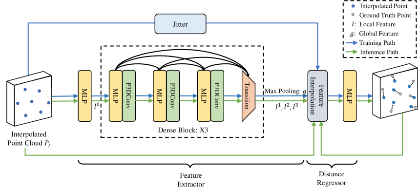
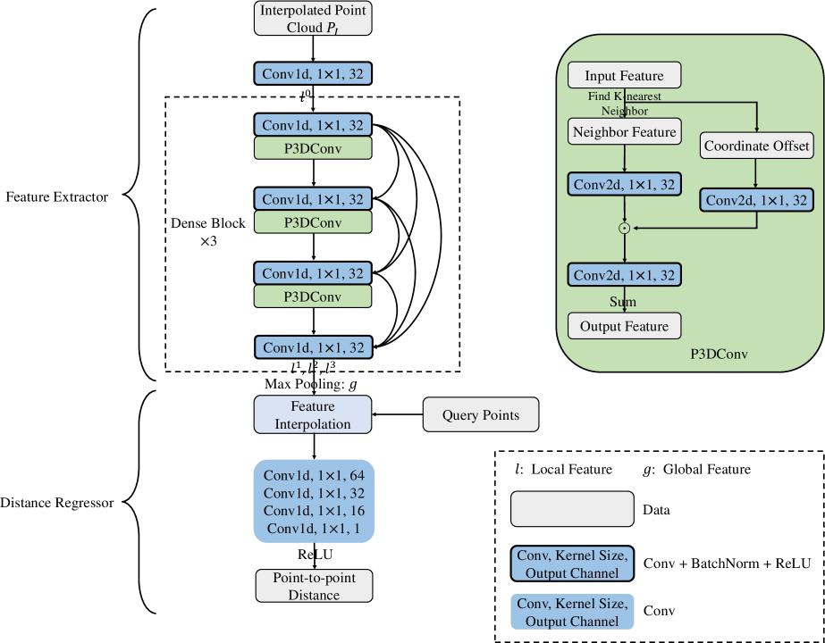
We design a Point-to-Point Distance Network (P2PNet) to approximate and serve as the oracle. In this section, we detail the design of P2PNet which mainly consists of a feature extractor and distance regressor, as in Fig 3.
Feature Extractor
To capture the local and global geometric information of irregular points, we adopt the Point 4D Convolution from P4Transformer [6], but simplify it to apply on the spatial domain only, thus termed as Point 3D Convolution (P3DConv). Specifically, for each interpolated point and its associated feature , we first search for its -nearest neighbor , and calculate the coordinate offset between them for convolution kernel generation. Then the P3DConv on interpolated point is conducted as follow:
| (2) |
where is the convoluted feature, is the -nearest neighbor set of point , all indicate an MLP-based transformation with the same output channel , and represents the Hadamard product.
The detailed structure of our feature extractor is shown in Fig 3. Given an interpolated point cloud , where is the number of points, an MLP first projects to a higher dimensional space , followed by a stack of three dense blocks with intra-block dense connection [13]. Each dense block consists of three convolution groups, followed by a transition down layer. Inside each convolutional group, an MLP reduces the feature dimension, while a P3DConv layer extracts local features. The transition down layer is another MLP that reduces the feature channels and therefore following computational cost. All MLPs for feature extraction share the same output channel of . In the end, a set of multi-scale local features is captured. By further applying a max pooling layer, a global feature is obtained.
Distance Regressor
For any query point , its point-to-point distance is estimated based on the extracted local features and global feature .
To obtain the point-wise local features for each query point , we follow [28] to conduct the feature interpolation, using the inverse distances of three-nearest neighbors in the initial interpolated point cloud as weights. With that, the point-to-point distance can be estimated as follow:
| (3) |
where are the interpolated multi-scale local features, is the global feature, and is a four-layer MLP.
Inference
During inference, the extracted local and global features are fixed. However in each iteration, since the points have moved, interpolated features are re-generated, thus new can be estimated.
Training
Unlike inference, there is no iterative optimization during training. Instead the interpolated points are jittered with Gaussian noise to serve as query points, which simulates varying degrees of displacement in different iterations, and increases the smoothness and continuity of learned distance functions.
Loss Function
We apply L1 loss to minimize the error between the predicted distance and the ground truth .
| (4) |
4 Evaluation
In this section, we first demonstrate the superior performance of our algorithm against prior state-of-the-arts on public datasets. And then validate the performance gain on downstream applications. Stress test results are also reported to demonstrate the robustness. Finally, we provide comprehensive ablation studies to prove the effectiveness of each component. Please refer to the supplementary material for implementation details and more comparative results.
4.1 Experiment Setup
Datasets
Two public datasets, PU-GAN [16] and PU1K [29] are used for evaluation. We follow the official training/testing splits and settings in original papers, where training is conducted on patch level. Compared to the PU-GAN dataset, PU1K is more challenging because it has a larger volume of data and more diverse categories.
During training, each input low-res patch contains points, while its corresponding high-res patch has points. Thus the upsampling rate . During testing, we follow [29] to generate point clouds from the test set of PU-GAN with Poisson disk sampling [46], as it only provides 3D meshes. All testing low-res point clouds from both datasets have points, while the high-res counterparts contain points. Given the low-res input, we first generate the interpolated point cloud by our midpoint interpolation. Then we follow [29] to extract patches, apply gradient descent to update them, and finally merge them to obtain the full high-res output.
Evaluation Metrics
Baselines
For the PU-GAN dataset, we train PU-Net [45], MPU [43], PU-GAN [16], Dis-PU [17], PU-EVA [20], PU-GCN [29] and Neural Points (NePs) [8] with the default settings in the respective papers as baselines. For the PU1K dataset, we only choose PU-Net [45], MPU [43] PU-GCN [29] and PU-Transformer [29], following original papers.
4.2 Comparison with SOTA
Results on the PU-GAN Dataset
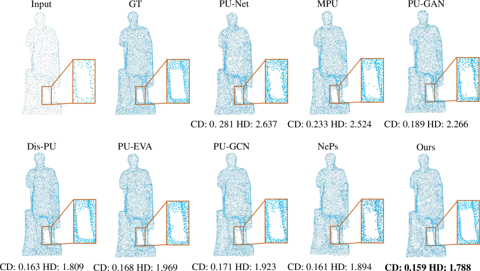
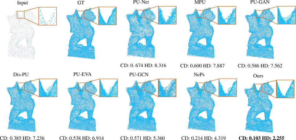
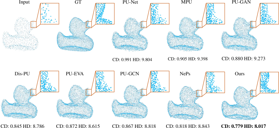
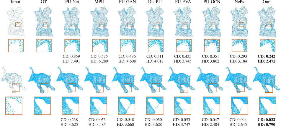
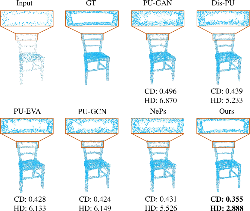
Tab 1 shows that our method outperforms prior arts on all metrics. In particular, the performance gain on higher upsampling rate () is larger. As shown in Fig 4, previous methods tend to generate outliers caused by overestimation of 3D coordinates. This artifact is more severe as the upsampling rate goes higher. On the contrary, our results have much less outliers, more faithful surfaces and more fine-grained details, without obvious distinction between and upsampling.
| Rates | ||||||||||||||||||||||||
|---|---|---|---|---|---|---|---|---|---|---|---|---|---|---|---|---|---|---|---|---|---|---|---|---|
| Methods |
|
|
|
|
|
|
|
|
||||||||||||||||
| PU-Net [45] | 0.529 | 6.805 | 4.760 | 814.3 | 0.566 | 0.510 | 8.206 | 6.041 | ||||||||||||||||
| MPU [43] | 0.292 | 6.672 | 2.822 | 76.2 | 0.573 | 0.219 | 7.054 | 3.085 | ||||||||||||||||
| PU-GAN [16] | 0.282 | 5.577 | 2.016 | 684.2 | 0.698 | 0.207 | 6.963 | 2.556 | ||||||||||||||||
| Dis-PU [17] | 0.274 | 3.696 | 1.943 | 1047.0 | 1.604 | 0.167 | 4.923 | 2.261 | ||||||||||||||||
| PU-EVA [20] | 0.277 | 3.971 | 2.524 | 2869.0 | 0.740 | 0.185 | 5.273 | 2.972 | ||||||||||||||||
| PU-GCN [29] | 0.268 | 3.201 | 2.489 | 76.0 | 0.538 | 0.161 | 4.283 | 2.632 | ||||||||||||||||
| NePs [8] | 0.259 | 3.648 | 1.935 | 664.1 | 0.403 | 0.152 | 4.910 | 2.198 | ||||||||||||||||
| Ours | 0.245 | 2.369 | 1.893 | 67.1 | 0.384 | 0.108 | 2.352 | 2.127 | ||||||||||||||||
In addition, we compare the efficiency of each method under setting, in terms of network parameters (Param.), as well as inference time which is measured end-to-end from loading the input low-res point cloud to generate the full high-res output, using a TITAN X GPU. Note that model size and inference time are not necessarily in proportion, because some of the expensive operations, e.g. -nearest neighbor search, are not part of the network. That said, our method is the fastest with the fewest parameters.
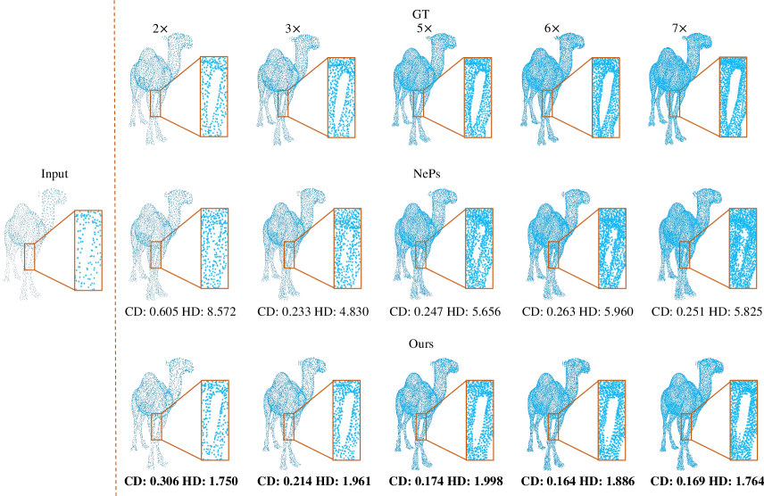
Arbitrary Upsampling Rates
Unlike most of previous methods [45, 16, 43, 17, 29, 30, 19, 32], our approach does not need retraining for different upsampling rates. Similarly, priort art NePs [8] also does not require retraining. Thus we conduct a comparison using the model trained on PU-GAN dataset. For both methods, we only vary the upsampling rate during inference while fixing all other parameters. Based on Tab 2, our method yields better accuracy under most of the metrics, except the P2F metric with and upsampling. Note that since P2F is asymmetrical, only from upsampled points to the ground truth surfaces but not vice versa[16], CD and HD metrics are more meaningful.
| Methods | NePs [8] | Ours | ||||||||||||||||
|---|---|---|---|---|---|---|---|---|---|---|---|---|---|---|---|---|---|---|
| Rates |
|
|
|
|
|
|
||||||||||||
| 0.642 | 7.324 | 2.574 | 0.540 | 3.177 | 1.775 | |||||||||||||
| 0.409 | 5.389 | 2.176 | 0.353 | 2.608 | 1.654 | |||||||||||||
| 0.248 | 3.922 | 1.871 | 0.234 | 2.549 | 1.836 | |||||||||||||
| 0.242 | 3.671 | 1.809 | 0.225 | 2.526 | 1.981 | |||||||||||||
| 0.237 | 3.796 | 1.795 | 0.219 | 2.634 | 1.940 | |||||||||||||
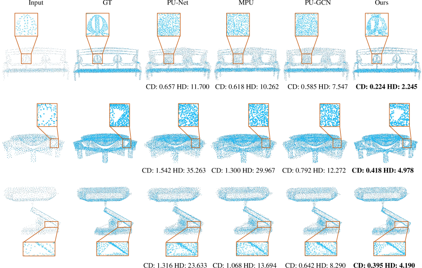
Results on the PU1K Dataset
We also conduct the evaluation on the more challenging PU1K dataset, as reported in Tab 3. Our method still outperforms others on almost all metrics, except for the P2F metric, which is second to PU-Transformer [32]. Note that our model is much smaller than PU-Transformer (67.1Kb vs. 969.9Kb).
| Methods |
|
|
|
||||||
|---|---|---|---|---|---|---|---|---|---|
| PU-Net [45] | 1.155 | 15.170 | 4.834 | ||||||
| MPU [43] | 0.935 | 13.327 | 3.511 | ||||||
| PU-GCN [29] | 0.585 | 7.577 | 2.499 | ||||||
| PU-Transformer [32] | 0.451 | 3.843 | 1.277 | ||||||
| Ours | 0.404 | 3.732 | 1.474 |
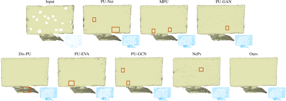
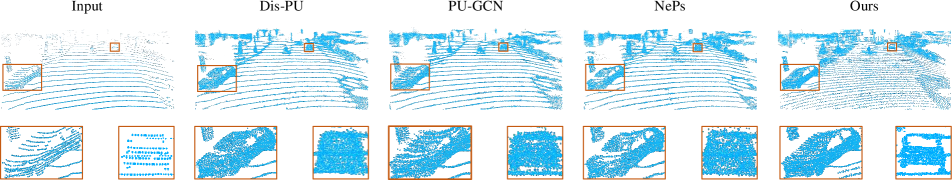
Results on Real Datasets
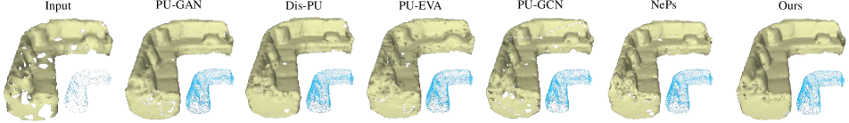
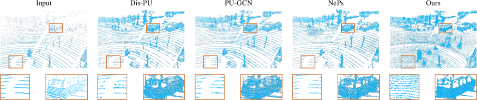
Using models trained on the PU-GAN dataset, we also conduct experiments on real-scanned point clouds from ScanObjectNN [35] and KITTI [9] datasets, as shown in Fig 5 and Fig 6. Since there is no ground truth high-res point cloud, we only qualitatively compare, and omit some methods that produce consistently worse results. Not only sparse and noisy, scanned data often have small holes or gaps, which makes them even more challenging. Fig 5 shows that our results are more complete, smooth and faithful, while other methods tend to keep the holes. In Fig 6, our result appears to be more complete and with more fine-grained details.
4.3 Impact on Downstream Tasks
We further highlight the upsampling quality in two downstream applications: point cloud classification and surface reconstruction.
Point Cloud Classification
We adopt CurveNet [40] as the classification model, and utilize the same training and testing schema on the ModelNet40 dataset [39]. Specifically, the model is trained with 1024 points. For each testing point cloud, we uniformly subsample 256 points as the low-res input, and upsample them back to 1024 points with various methods (trained on the PU-GAN dataset).
We then compare the classification performance on the downsampled low-res point clouds (Low-res, 256 points), original test set (High-res, 1024 points) and upsampled point clouds (1024 points). As shown in the first two rows of Tab 4, the classification accuracy of the low-res point clouds is observably worse, while our upsampling method brings a significant improvement.
| Classification Accuracy (%) | Low-res | High-res | PU-Net [45] | MPU [43] | PU-GAN [16] |
|---|---|---|---|---|---|
| 68.76 | 93.72 | 88.82 | 89.91 | 90.25 | |
| Dis-PU [17] | PU-EVA [20] | PU-GCN [29] | NePs [8] | Ours | |
| 91.57 | 90.83 | 91.21 | 91.39 | 91.96 | |
| Reconstruction CD () | Low-res | High-res | PU-Net [45] | MPU [43] | PU-GAN [16] |
| 0.106 | 0.039 | 0.221 | 0.102 | 0.090 | |
| Dis-PU [17] | PU-EVA [20] | PU-GCN [29] | NePs [8] | Ours | |
| 0.084 | 0.086 | 0.079 | 0.075 | 0.071 |
Surface Reconstruction
We utilize BallPivoting [1] to reconstruct meshes from the upsampled point clouds (8192 points) of PU-GAN dataset. From the last two rows of Tab 4, we find that the low-res point clouds (Low-res, 2048 points) already achieve a comparable performance, because they are directly sampled from the ground truth meshes. Although the improvement obtained by each method is marginal, our approach still yields the best.
4.4 Robustness Test
Additive Noise
As the point clouds captured by scanners are often noisy, it is necessary to evaluate the robustness of each method against noise. To be specific, we first generate some random noise offline, which is sampled from a standard Gaussian distribution and multiplied by a factor , where denotes the noise level. Then we test on the low-res point clouds of PU-GAN dataset with added noise. And the training of all methods incorporate with Gaussian noise perturbation as augmentation strategy for fair comparison. As shown in Tab 5, our method achieves the best performance consistently, especially at high noise level. And Fig 7 provides the qualitative comparisons, which verifies that our result is cleaner with much less outliers.
| Noise Levels | ||||||||||||||||||
|---|---|---|---|---|---|---|---|---|---|---|---|---|---|---|---|---|---|---|
| Methods |
|
|
|
|
|
|
||||||||||||
| PU-Net [45] | 0.628 | 8.068 | 9.816 | 1.078 | 10.867 | 16.401 | ||||||||||||
| MPU [43] | 0.506 | 6.978 | 9.059 | 0.929 | 10.820 | 15.621 | ||||||||||||
| PU-GAN [16] | 0.464 | 6.070 | 7.498 | 0.887 | 10.602 | 15.088 | ||||||||||||
| Dis-PU [17] | 0.419 | 5.413 | 6.723 | 0.818 | 9.345 | 14.376 | ||||||||||||
| PU-EVA [20] | 0.459 | 5.377 | 7.189 | 0.839 | 9.325 | 14.652 | ||||||||||||
| PU-GCN [29] | 0.448 | 5.586 | 6.989 | 0.816 | 8.604 | 13.798 | ||||||||||||
| NePs [8] | 0.425 | 5.438 | 6.546 | 0.798 | 9.102 | 12.088 | ||||||||||||
| Ours | 0.414 | 4.145 | 6.400 | 0.766 | 7.339 | 11.534 | ||||||||||||
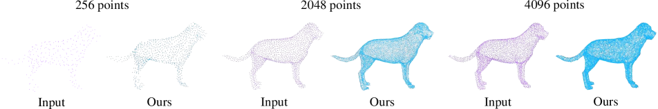
Various Input Sizes
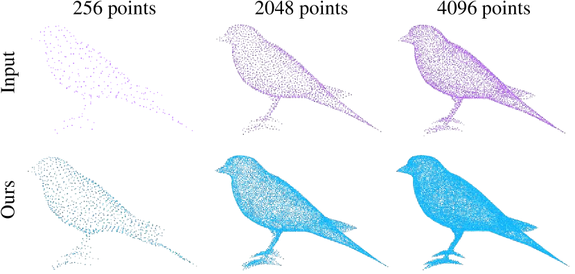
Considering all previous evaluations of PU-GAN and PU1K datasets are conducted on the low-res point clouds with 2048 points, we further validate the robustness of our method against different input sizes. As Fig 8 shows, although our model is trained on the fixed-scale input data, it can generalize well to different scales during inference, even when the input is extremely sparse.
4.5 Ablation Study
In this section, we conduct the comprehensive ablation studies to validate the effectiveness of each component, and all these experiments are based on the PU1K dataset with setting.
Distance Regression vs. Coordinate Prediction
Compared with predicting 3D coordinates or residuals, merely regressing the point-to-point distance is a relatively easier task. To verify this point, we modify the output channel of P2PNet’s last MLP to predict the 3D coordinate offset for each interpolated point, and we employ a L2 loss to minimize the prediction error. Following [21, 41, 22], we update the interpolated points to ground truth locations in an auto-regression way:
| (5) |
where denotes the predicted coordinate displacement, is the step size, and we fine-tune it and iteration number to achieve the best performance, holding all other parameters the same. Moreover, we also report the results of end-to-end update, which repeats Eq 5 only once with step size .
| Prediction Contents |
|
|
|
||||||
|---|---|---|---|---|---|---|---|---|---|
| 3D Coordinate Offset (End-to-end) | 1.170 | 11.834 | 2.521 | ||||||
| 3D Coordinate Offset (Auto-regression) | 0.663 | 7.034 | 1.935 | ||||||
| Point-to-point Distance | 0.404 | 3.732 | 1.474 |
As reported in Tab 6, our distance regression based method clearly achieves superior performance, although updating points auto-regressively can alleviate the misestimation of predicted coordinate offsets to some extent.
Midpoint Interpolation
We employ the midpoint interpolation result to serve as both input of P2PNet and initial point cloud to be updated. For validating the effectiveness of midpoint interpolation, we replace the input of P2PNet with the low-res point cloud . And we also sample points from the Gaussian distribution to get another initial point cloud, denoted as . Finally, we combine different network inputs and initial point clouds to conduct the experiments, holding all other parameters the same.
| Network Inputs | Initial Point Clouds to Be Updated |
|
|
|
||||||
|---|---|---|---|---|---|---|---|---|---|---|
| 0.713 | 5.586 | 1.656 | ||||||||
| 0.426 | 3.989 | 1.813 | ||||||||
| 0.654 | 5.295 | 1.616 | ||||||||
| 0.404 | 3.732 | 1.474 |
From the second and forth rows of Tab 7, we conclude that using the denser interpolated point cloud as network input can achieve better performance, since it contains more geometrical information and benefits the feature extraction process. And the improvement is more evident in the comparison between the third and forth rows, it proves that our midpoint interpolation result provides a better initial position, which benefits the update process under the same number of iterations.
P3DConv vs. EdgeConv [43]
The EdgeConv based feature extractor [43] is widely used by previous work [16, 17, 43, 8, 48]. However, EdgeConv [43] utilizes most of parameters to refine each individual feature. While our P3DConv focuses on the feature aggregation achieved by generated convolution kernels, thus benefits the extraction of local and global features. For verifying the superior performance of our P3DConv, we replace the dense block in our P2PNet with EdgeConv in [43], and we also fine-tune the number of EdgeConv layers to achieve the comparable network parameters, as Tab 8 shows.
5 Conclusion
We propose a novel method for precise point cloud upsampling, supporting arbitrary upsampling rates after training once. For arbitrary upsampling rates, we propose to directly upsample points in Euclidean space via midpoint interpolation and then refine them, which decouples the point generation from network learning. For refining the interpolated points more precisely, we regard the refinement as an optimization problem, and then solve it by minimizing the learned point-to-point distance function. And considering the ground truth point cloud is not avaliable during inference, we construct P2PNet to approximate the point-to-point distance function in a differentiable way. Extensive quantitative and qualitative comparisons on benchmarks and downstream tasks demonstrate that our method outperforms prior state-of-the-art methods, while achieving the fewest parameters and fastest inference speed.
Acknowledgments
This work was supported in part by NSFC Project (62176061) and STCSM Project (No.22511105000). Danhang Tang, Yinda Zhang and Xiangyang Xue are the corresponding authours.
References
- [1] Fausto Bernardini, Joshua Mittleman, Holly Rushmeier, Cláudio Silva, and Gabriel Taubin. The ball-pivoting algorithm for surface reconstruction. IEEE transactions on visualization and computer graphics, 5(4):349–359, 1999.
- [2] Zhiqin Chen and Hao Zhang. Learning implicit fields for generative shape modeling. In Proceedings of the IEEE/CVF Conference on Computer Vision and Pattern Recognition, pages 5939–5948, 2019.
- [3] Julian Chibane, Thiemo Alldieck, and Gerard Pons-Moll. Implicit functions in feature space for 3d shape reconstruction and completion. In Proceedings of the IEEE/CVF Conference on Computer Vision and Pattern Recognition, pages 6970–6981, 2020.
- [4] Julian Chibane, Gerard Pons-Moll, et al. Neural unsigned distance fields for implicit function learning. Advances in Neural Information Processing Systems, 33:21638–21652, 2020.
- [5] Peng Dai, Yinda Zhang, Zhuwen Li, Shuaicheng Liu, and Bing Zeng. Neural point cloud rendering via multi-plane projection. In Proceedings of the IEEE/CVF Conference on Computer Vision and Pattern Recognition, pages 7830–7839, 2020.
- [6] Hehe Fan, Yi Yang, and Mohan Kankanhalli. Point 4d transformer networks for spatio-temporal modeling in point cloud videos. In Proceedings of the IEEE/CVF Conference on Computer Vision and Pattern Recognition, pages 14204–14213, 2021.
- [7] Hehe Fan, Xin Yu, Yuhang Ding, Yi Yang, and Mohan Kankanhalli. Pstnet: Point spatio-temporal convolution on point cloud sequences. arXiv preprint arXiv:2205.13713, 2022.
- [8] Wanquan Feng, Jin Li, Hongrui Cai, Xiaonan Luo, and Juyong Zhang. Neural points: Point cloud representation with neural fields for arbitrary upsampling. In Proceedings of the IEEE/CVF Conference on Computer Vision and Pattern Recognition, pages 18633–18642, 2022.
- [9] Andreas Geiger, Philip Lenz, Christoph Stiller, and Raquel Urtasun. Vision meets robotics: The kitti dataset. The International Journal of Robotics Research, 32(11):1231–1237, 2013.
- [10] Amos Gropp, Lior Yariv, Niv Haim, Matan Atzmon, and Yaron Lipman. Implicit geometric regularization for learning shapes. arXiv preprint arXiv:2002.10099, 2020.
- [11] Yulan Guo, Hanyun Wang, Qingyong Hu, Hao Liu, Li Liu, and Mohammed Bennamoun. Deep learning for 3d point clouds: A survey. IEEE transactions on pattern analysis and machine intelligence, 43(12):4338–4364, 2020.
- [12] Yun He, Xinlin Ren, Danhang Tang, Yinda Zhang, Xiangyang Xue, and Yanwei Fu. Density-preserving deep point cloud compression. In Proceedings of the IEEE/CVF Conference on Computer Vision and Pattern Recognition, pages 2333–2342, 2022.
- [13] Gao Huang, Zhuang Liu, Laurens Van Der Maaten, and Kilian Q Weinberger. Densely connected convolutional networks. In Proceedings of the IEEE conference on computer vision and pattern recognition, pages 4700–4708, 2017.
- [14] Chiyu Jiang, Avneesh Sud, Ameesh Makadia, Jingwei Huang, Matthias Nießner, Thomas Funkhouser, et al. Local implicit grid representations for 3d scenes. In Proceedings of the IEEE/CVF Conference on Computer Vision and Pattern Recognition, pages 6001–6010, 2020.
- [15] Diederik P Kingma and Jimmy Ba. Adam: A method for stochastic optimization. arXiv preprint arXiv:1412.6980, 2014.
- [16] Ruihui Li, Xianzhi Li, Chi-Wing Fu, Daniel Cohen-Or, and Pheng-Ann Heng. Pu-gan: a point cloud upsampling adversarial network. In Proceedings of the IEEE/CVF International Conference on Computer Vision, pages 7203–7212, 2019.
- [17] Ruihui Li, Xianzhi Li, Pheng-Ann Heng, and Chi-Wing Fu. Point cloud upsampling via disentangled refinement. In Proceedings of the IEEE/CVF Conference on Computer Vision and Pattern Recognition, pages 344–353, 2021.
- [18] Yangyan Li, Rui Bu, Mingchao Sun, Wei Wu, Xinhan Di, and Baoquan Chen. Pointcnn: Convolution on x-transformed points. Advances in neural information processing systems, 31, 2018.
- [19] Chen Long, WenXiao Zhang, Ruihui Li, Hao Wang, Zhen Dong, and Bisheng Yang. Pc2-pu: Patch correlation and point correlation for effective point cloud upsampling. In Proceedings of the 30th ACM International Conference on Multimedia, pages 2191–2201, 2022.
- [20] Luqing Luo, Lulu Tang, Wanyi Zhou, Shizheng Wang, and Zhi-Xin Yang. Pu-eva: An edge-vector based approximation solution for flexible-scale point cloud upsampling. In Proceedings of the IEEE/CVF International Conference on Computer Vision, pages 16208–16217, 2021.
- [21] Shitong Luo and Wei Hu. Score-based point cloud denoising. In Proceedings of the IEEE/CVF International Conference on Computer Vision, pages 4583–4592, 2021.
- [22] Wei-Chiu Ma, Shenlong Wang, Jiayuan Gu, Sivabalan Manivasagam, Antonio Torralba, and Raquel Urtasun. Deep feedback inverse problem solver. In Computer Vision–ECCV 2020: 16th European Conference, Glasgow, UK, August 23–28, 2020, Proceedings, Part V 16, pages 229–246. Springer, 2020.
- [23] Daniel Maturana and Sebastian Scherer. Voxnet: A 3d convolutional neural network for real-time object recognition. In 2015 IEEE/RSJ International Conference on Intelligent Robots and Systems (IROS), pages 922–928. IEEE, 2015.
- [24] Lars Mescheder, Michael Oechsle, Michael Niemeyer, Sebastian Nowozin, and Andreas Geiger. Occupancy networks: Learning 3d reconstruction in function space. In Proceedings of the IEEE/CVF conference on computer vision and pattern recognition, pages 4460–4470, 2019.
- [25] Jeong Joon Park, Peter Florence, Julian Straub, Richard Newcombe, and Steven Lovegrove. Deepsdf: Learning continuous signed distance functions for shape representation. In Proceedings of the IEEE/CVF Conference on Computer Vision and Pattern Recognition, pages 165–174, 2019.
- [26] Adam Paszke, Sam Gross, Francisco Massa, Adam Lerer, James Bradbury, Gregory Chanan, Trevor Killeen, Zeming Lin, Natalia Gimelshein, Luca Antiga, et al. Pytorch: An imperative style, high-performance deep learning library. Advances in neural information processing systems, 32, 2019.
- [27] Charles R Qi, Hao Su, Kaichun Mo, and Leonidas J Guibas. Pointnet: Deep learning on point sets for 3d classification and segmentation. In Proceedings of the IEEE conference on computer vision and pattern recognition, pages 652–660, 2017.
- [28] Charles Ruizhongtai Qi, Li Yi, Hao Su, and Leonidas J Guibas. Pointnet++: Deep hierarchical feature learning on point sets in a metric space. Advances in neural information processing systems, 30, 2017.
- [29] Guocheng Qian, Abdulellah Abualshour, Guohao Li, Ali Thabet, and Bernard Ghanem. Pu-gcn: Point cloud upsampling using graph convolutional networks. In Proceedings of the IEEE/CVF Conference on Computer Vision and Pattern Recognition, pages 11683–11692, 2021.
- [30] Yue Qian, Junhui Hou, Sam Kwong, and Ying He. Pugeo-net: A geometry-centric network for 3d point cloud upsampling. In European Conference on Computer Vision, pages 752–769. Springer, 2020.
- [31] Yue Qian, Junhui Hou, Sam Kwong, and Ying He. Deep magnification-flexible upsampling over 3d point clouds. IEEE Transactions on Image Processing, 30:8354–8367, 2021.
- [32] Shi Qiu, Saeed Anwar, and Nick Barnes. Pu-transformer: Point cloud upsampling transformer. arXiv preprint arXiv:2111.12242, 2021.
- [33] Gernot Riegler, Ali Osman Ulusoy, and Andreas Geiger. Octnet: Learning deep 3d representations at high resolutions. In Proceedings of the IEEE conference on computer vision and pattern recognition, pages 3577–3586, 2017.
- [34] Sebastian Ruder. An overview of gradient descent optimization algorithms. arXiv preprint arXiv:1609.04747, 2016.
- [35] Mikaela Angelina Uy, Quang-Hieu Pham, Binh-Son Hua, Thanh Nguyen, and Sai-Kit Yeung. Revisiting point cloud classification: A new benchmark dataset and classification model on real-world data. In Proceedings of the IEEE/CVF international conference on computer vision, pages 1588–1597, 2019.
- [36] Ashish Vaswani, Noam Shazeer, Niki Parmar, Jakob Uszkoreit, Llion Jones, Aidan N Gomez, Łukasz Kaiser, and Illia Polosukhin. Attention is all you need. Advances in neural information processing systems, 30, 2017.
- [37] Yue Wang, Yongbin Sun, Ziwei Liu, Sanjay E Sarma, Michael M Bronstein, and Justin M Solomon. Dynamic graph cnn for learning on point clouds. Acm Transactions On Graphics (tog), 38(5):1–12, 2019.
- [38] Wenxuan Wu, Zhongang Qi, and Li Fuxin. Pointconv: Deep convolutional networks on 3d point clouds. In Proceedings of the IEEE/CVF Conference on Computer Vision and Pattern Recognition, pages 9621–9630, 2019.
- [39] Zhirong Wu, Shuran Song, Aditya Khosla, Fisher Yu, Linguang Zhang, Xiaoou Tang, and Jianxiong Xiao. 3d shapenets: A deep representation for volumetric shapes. In Proceedings of the IEEE conference on computer vision and pattern recognition, pages 1912–1920, 2015.
- [40] Tiange Xiang, Chaoyi Zhang, Yang Song, Jianhui Yu, and Weidong Cai. Walk in the cloud: Learning curves for point clouds shape analysis. In Proceedings of the IEEE/CVF International Conference on Computer Vision, pages 915–924, 2021.
- [41] Yu Xiang, Tanner Schmidt, Venkatraman Narayanan, and Dieter Fox. Posecnn: A convolutional neural network for 6d object pose estimation in cluttered scenes. arXiv preprint arXiv:1711.00199, 2017.
- [42] Shuquan Ye, Dongdong Chen, Songfang Han, Ziyu Wan, and Jing Liao. Meta-pu: An arbitrary-scale upsampling network for point cloud. IEEE transactions on visualization and computer graphics, 2021.
- [43] Wang Yifan, Shihao Wu, Hui Huang, Daniel Cohen-Or, and Olga Sorkine-Hornung. Patch-based progressive 3d point set upsampling. In Proceedings of the IEEE/CVF Conference on Computer Vision and Pattern Recognition, pages 5958–5967, 2019.
- [44] Lequan Yu, Xianzhi Li, Chi-Wing Fu, Daniel Cohen-Or, and Pheng-Ann Heng. Ec-net: an edge-aware point set consolidation network. In Proceedings of the European conference on computer vision (ECCV), pages 386–402, 2018.
- [45] Lequan Yu, Xianzhi Li, Chi-Wing Fu, Daniel Cohen-Or, and Pheng-Ann Heng. Pu-net: Point cloud upsampling network. In Proceedings of the IEEE conference on computer vision and pattern recognition, pages 2790–2799, 2018.
- [46] Cem Yuksel. Sample elimination for generating poisson disk sample sets. In Computer Graphics Forum, volume 34, pages 25–32. Wiley Online Library, 2015.
- [47] Hengshuang Zhao, Li Jiang, Jiaya Jia, Philip HS Torr, and Vladlen Koltun. Point transformer. In Proceedings of the IEEE/CVF International Conference on Computer Vision, pages 16259–16268, 2021.
- [48] Wenbo Zhao, Xianming Liu, Zhiwei Zhong, Junjun Jiang, Wei Gao, Ge Li, and Xiangyang Ji. Self-supervised arbitrary-scale point clouds upsampling via implicit neural representation. In Proceedings of the IEEE/CVF Conference on Computer Vision and Pattern Recognition, pages 1999–2007, 2022.
Supplementary Material
In this supplementary material, we provide additional implementation details, ablation studies and qualitative results.
1 Implementation Details
Additional details about hyperparameter settings and detailed network architecture are elucidated in this section.
1.1 Hyperparameters
In the P2PNet, we set the feature dimension and the nearest neighbor number . For training, we use random perturbation, rotation and scaling for data augmentation, the same as [29]. For testing, we choose the iteration number to balance the computational cost and performance.
1.2 Detailed Network Architecture
The detailed architecture of our P2PNet is shown in Fig 9. In the feature extractor, we first employ an MLP to project the initial interpolated point cloud to a higher dimension space. And then stack three dense blocks with intra-block dense connection [13], where each block comprises four MLPs and three P3DConv layers. The MLP is used to reduce feature channel, and the P3DConv layer is utilized for local feature capture. Lastly, we obtain the extracted local features as well as global feature . In the distance regressor, we first get the point-wise local features of query point by feature interpolation [28], and then apply a four-layer MLP to regress the point-to-point distance. The formula of feature interpolation [28] at point is listed below:
| (6) |
where () are the interpolated multi-scale local features, () are the three nearest-neighbors of query point in the initial interpolated point cloud, and is the distance between and .
2 Additional Ablation Studies
In this section, we conduct more ablation experiments to validate our choices of regressor input, training scheme with Gaussian noise and location refinement strategy. All the evaluations are done on the PU1K dataset with upsampling.
Regressor Input
In our full model, we regress the point-to-point distance of each query point using the concatenation of coordinate , interpolated local features and global feature . We here analyze the impact of each type of feature on the final performance. We train models with either local feature or global feature, and show their performances in Tab 9. Both cases perform worse than our full model, which uses both features.
| Regressor Inputs |
|
|
|
||||||
|---|---|---|---|---|---|---|---|---|---|
| 0.729 | 8.439 | 2.324 | |||||||
| 0.423 | 4.011 | 1.652 | |||||||
| 0.404 | 3.732 | 1.474 |
Training Scheme with Gaussian Noise
During training, we jitter the interpolated points with Gaussian noise to obtain query points, which simulates the iterative optimization process of inference. To verify the effectiveness of this training scheme, we train our P2PNet with or without Gaussian noise, while sharing the same testing process. As shown in Tab 10, using Gaussian noise for training achieves superior performance, since it simulates the upsampling error from not just the initial interpolated point cloud but all iterations, and also increases the smoothness and continuity of learned distance functions.
|
|
|
|
|||||||
|---|---|---|---|---|---|---|---|---|---|---|
| w/o Gaussian Noise | 0.520 | 5.368 | 1.729 | |||||||
| w Gaussian Noise | 0.404 | 3.732 | 1.474 |
Location Refinement Strategy
After midpoint interpolation, we iteratively move the interpolated point towards the ground truth position, guided by the estimated point-to-point distance and predefined step size , as formulated below:
| (7) |
where , is the predefined iteration number.
And Chibane et al. [4] also propose to project point by moving it the predicted distance along the normalized negative gradient, as listed below:
| (8) |
We use Eq 7 and Eq 8 as the refinement strategy respectively, and we also fine-tune the iteration number for Eq 8 to achieve the best performance. As shown in Tab 11, our Eq 7 is much more accurate than Eq 8. While Eq 8 requires that the estimated distance and direction should be both accurate enough to achieve a good performance. Our Eq 7 only requires the accuracy of the direction. And once the direction is precisely predicted, the convergence of the interpolated point can be guaranteed, given sufficient iterations and a suitable step size [21].
3 Additional Qualitative Results
In this section, we show some more qualitative results on the PU-GAN [16], PU1K [29], ScanObjectNN [35] and KITTI [9] datasets, which further validate that our method achieves superior upsampling quality. Specifically, in Fig 10 and Fig 11, we provide more visual comparisons with previous SOTA methods on the PU-GAN dataset, under and settings respectively. In Fig 12, we visualize the upsampled results with various upsampling rates after one-time training. In Fig 13, we present qualitative comparisons on the PU1K dataset with setting. In Fig 14 and Fig 15, we employ added noise and different input sizes to verify the robustness of our method. In Fig 16 and Fig 17, we display more qualitative results on the real-scanned inputs. Consistent with the main paper, we use CD and HD to represent Chamfer distance and Hausdorff distance respectively, while their units are both .