GPS Spoofing Mitigation and Timing Risk Analysis in Networked PMUs via Stochastic Reachability
BIOGRAPHIES
Sriramya Bhamidipati is a Ph.D. student in the Department of Aerospace Engineering at the University of Illinois at Urbana-Champaign, where she also received her master’s degree in 2017. She obtained her B.Tech. in Aerospace from the Indian Institute of Technology, Bombay in 2015. Her research interests include GPS, power and control systems, artificial intelligence, computer vision, and unmanned aerial vehicles.
Grace Xingxin Gao is an assistant professor in the Department of Aeronautics and Astronautics at Stanford University. Before joining Stanford University, she was an assistant professor at University of Illinois at Urbana-Champaign. She obtained her Ph.D. degree at Stanford University. Her research is on robust and secure positioning, navigation and timing with applications to manned and unmanned aerial vehicles, robotics, and power systems.
ABSTRACT
To address PMU vulnerability against spoofing, we propose a set-valued state estimation technique known as Stochastic Reachability-based Distributed Kalman Filter (SR-DKF) that computes secure GPS timing across a network of receivers. Utilizing stochastic reachability, we estimate not only GPS time but also its stochastic reachable set, which is parameterized via probabilistic zonotope (p-Zonotope). While requiring known measurement error bounds in only non-spoofed conditions, we design a two-tier approach: We first perform measurement-level spoofing mitigation via deviation of measurement innovation from its expected p-Zonotope, and second perform state-level timing risk analysis via intersection probability of estimated p-Zonotope with an unsafe set that violates IEEE C37.118.1a-2014 standards. We validate the proposed SR-DKF by subjecting a simulated receiver network to coordinated signal-level spoofing. We demonstrate an improved GPS timing accuracy and successful spoofing mitigation via our SR-DKF. We validate the robustness of the estimated timing risk as the number of receivers are varied.
1 INTRODUCTION
Modern power systems analyze real-time grid stability using a widely dispersed network of advanced devices, known as Phasor Measurement Units (PMUs) [1]. As per the American Recovery and Reinvestment Act of , almost PMUs have been deployed across the US and Canada as of March [2, 3]. Figure 1 shows a map of the dense network of these spatially distributed PMUs. The North American Synchrophasor Initiative network (NASPInet), which is a collaborative effort by the U.S. Department of Energy and the North American Electric Reliability Corporation, provides a secure and decentralized infrastructure for communication among the PMUs [4]. Each PMU is equipped with a GPS receiver to precisely time-stamp the voltage and current phasor values at critical power substations. A network of geographically distributed GPS receivers facilitate robust time authentication by cross-checking each other and thereby eliminate the need for an external reference receiver [5]. The networked approach in power systems overlays the existing grid infrastructure and therefore can be implemented without additional hardware.
PMUs are susceptible to GPS spoofing because of the low signal power and unencrypted structure of the civilian GPS/L1 signals [6]. As validated in prior literature [7], this vulnerability can be exploited by attackers to mislead the GPS timing at one or more critical substations and cause cascading system failure. The various spoofing attacks that can potentially disrupt GPS timing vary from a simple meaconing to more sophisticated signal-level spoofing and coordinated attacks. A spoofer executing meaconing (or time jump) broadcasts earlier recorded authentic GPS signals to induce a constant lag in the victim receiver’s computed time as compared to the true time. In signal-level spoofing (or time walk), the spoofer broadcasts the simulated GPS signals to gradually steer the computed time of victim receiver away from its true time. In addition, coordinated attack occurs when multiple spoofers manipulate the GPS signals received at one or more victim receivers. We refer readers to our prior work for a detailed overview of these attacks [8].
Secure GPS timing is of paramount importance for reliable PMU operations. The IEEE C37.118.1a-2014 standards for Synchrophasors [9] define % Total Vector Error (TVE) as a benchmark for grid stability. For a PMU operating at Hz, which is a commonly used frequency for phasor data logging, % TVE is caused by a timing error of s. The key measures of secure GPS timing are spoofing attack mitigation and timing risk analysis. In this context, we define risk as the probability of estimation error to exceed a safety Alert Limit (AL). In this work, we set s to ensure that the estimation error in GPS time complies with the IEEE C37.118.1a-2014 standards.

The state-of-the-art prior work [11, 12, 13] on networked anti-spoofing falls under the category of point-valued state estimation approaches. A point-valued state estimate denotes the expected value of the state vector given the measurements. The existing literature on the point-valued anti-spoofing methods, which is summarized in [14, 15, 8], includes signal quality monitoring, angle-of-arrival and time-difference-of-arrival-based analyses of the incoming satellite signals, validation of the encryption codes, and attack magnitude estimation. Unlike the point-valued techniques, a set-valued approach utilizes the pre-computed (or known) error bounds on system dynamics and received measurements to propagate the set of state estimates [16]. An illustration of the difference between point-valued and set-valued propagation is seen in Fig. 2(a).


Much prior literature is available on set-valued theory [16, 17, 18]. Our current work is inspired by a set-valued formulation designed for stochastic processes known as stochastic reachability [19]. Stochastic reachability is widely used in robotics for path planning and collision avoidance, however, it has not been applied in the field of power systems. As shown in Fig. 2(b), stochastic reachability computes a set of stochastic reachable states given an initial stochastic set of states, and the known stochastic sets of system disturbances and measurement errors. In this context, each state in the stochastic reachable set is associated with a probabilistic measure that indicates the likelihood of its occurrence. Our choice of stochastic reachability is justified because it accounts for the stochastic errors in receiver clock dynamics, data transfer latencies, and GPS measurements.
In this work, we propose a set-valued state estimation technique for a network of GPS receivers, termed as Stochastic Reachability-based Distributed Kalman Filter (SR-DKF). The stochastic reachability formulation requires known error bounds, however, the attack errors induced via spoofing are unbounded and time-varying in nature. To account for this, we consider the error bounds in GPS measurements to be known only in non-spoofed (or authentic) conditions and pre-compute these bounds from offline empirical analysis of historical data [20]. This current work is based on our recent ION GNSS+ conference paper [21].
In a conventional DKF approach [22], each receiver evaluates the received measurements against a point-valued attack threshold and thereafter fuses the measurements obtained from different receivers to compute its point-valued state estimate. In contrast, our SR-DKF performs secure state estimation of GPS time and spoofing attack mitigation in the set-valued domain. Therefore, we estimate not only the point-valued mean but also the stochastic reachable set of GPS time that is later utilized to compute the associated risk of violating IEEE C37.118.1a-2014 standards. Unlike the point-valued state estimation techniques [12, 8], our proposed SR-DKF algorithm does not require the conservative assumption that all satellite measurements at a victim receiver are attacked by the spoofer. Our set-valued analysis of spoofing attack combined with the redundancy in number of available measurements from a network of GPS receivers, eliminates the need to estimate the attack magnitude [23]. To our knowledge, no prior literature exists on performing the secure state estimation using stochastic reachability nor on quantifying the timing risk associated with estimated GPS time.
1.1 Contributions
The main contributions of this paper are listed as follows:
-
1.
Utilizing an efficient set representation known as probabilistic zonotope (p-Zonotope) [24] to parameterize the stochastic reachable set, we develop a set-valued DKF framework to compute secure GPS time for a network of receivers.
-
2.
Considering offline-estimated measurement error bounds in non-spoofed (or authentic) conditions, we design a two-tier approach that performs
-
(a)
Measurement-level spoofing attack mitigation by adaptively evaluating the deviation of point-valued GPS measurements from the set-valued domain of measurement innovation. Therefore, the proposed SR-DKF algorithm is resilient to a variety of GPS attacks, such as meaconing, signal-level spoofing, coordinated attack, etc.
-
(b)
State-level timing risk analysis by estimating the intersection probability of the estimated set of stochastic reachable states (represented by p-Zonotope) with an unsafe set, i.e., a set violating the IEEE C37.118.1a-2014 standards [9].
-
(a)
-
3.
For a simulated setup, we demonstrate the successful mitigation of both simple meaconing and sophisticated signal-level spoofing attacks. During a simulated case of coordinated attack that affects multiple receivers, we show an improvement in the state estimation accuracy via the proposed SR-DKF algorithm as compared to conventional point-valued DKF and single-receiver-based adaptive KF. We also demonstrate the robustness of the proposed SR-DKF algorithm by analyzing the variation in timing risk with respect to the number of receivers and magnitude of spoofing attacks.
The rest of the paper is organized as follows: Section 2 outlines the system model, the preliminaries of stochastic reachability and the conventional point-valued DKF; Section 3 describes the proposed SR-DKF algorithm; Section 4 experimentally validates the improved state estimation accuracy of the GPS timing computed via SR-DKF as compared to the point-valued DKF, and also demonstrates the trend of timing risk associated with the estimated GPS time; and Section 5 concludes the paper.
2 PROBLEM FORMULATION
The three main design aspects of the proposed SR-DKF algorithm, namely i) a spatially distributed network of static GPS receivers, ii) a distributed processing framework, and iii) the set representation via p-Zonotopes, are described as follows:
i) A spatially distributed network of static GPS receivers:
We utilize the existing grid infrastructure to consider a handful (around four to eight) of the spatially distributed PMUs (or GPS receivers). This framework provides two advantages: First, by considering a spatially distributed network, we increase the measurement redundancy while minimizing the probability of multiple receivers being simultaneously spoofed; Second, given that the power substations are static, we can utilize the known receiver positions to aid the proposed SR-DKF algorithm.
ii) A distributed processing framework:
We opt for distributed processing to minimize the reaction time to attacks and also to localize the extent of failure. This is justified because global GPS reference time for synchronizing the PMUs is no longer reliable during spoofing. Therefore, the conventional communication protocol involving send or receive requests cannot be scheduled across the network. Each receiver in our distributed network asynchronously broadcasts the latest data to its neighbors, thereby reducing communication latency.


iii) The set representation via p-Zonotopes:
We represent stochastic reachable set via an enclosing probabilistic hull [24] known as p-Zonotope, denoted by . Among all available set representations [26] such as zonotope, ellipsoid, polytope, etc., our choice of p-Zonotope is justified because it can efficiently enclose the stochastic biases in GPS measurements. A p-Zonotope can enclose a variety of distributions such as mixture models, distributions with uncertain/time-dependent mean, non-Gaussian/unknown distribution, etc. A one-Dimensional (1D) example of a p-Zonotope that encloses multiple Gaussian distributions with varying mean and covariance is illustrated in Fig. 3(a). The probabilistic nature of p-Zonotopes blends well with the Gaussian-centric framework of DKF.
Unlike the conventional techniques that propagate point-valued state estimates, the proposed SR-DKF algorithm utilizes the pre-computed error bounds on the receiver clock dynamics and measurements to recursively propagate the p-Zonotope of the state estimate. An example of a two-Dimensional (2D) p-Zonotope is shown in Fig. 3(b). In this work, the 2D p-Zonotope is used to represent the state estimate that is introduced later in Section 3.
2.1 Preliminaries of p-Zonotopes
A p-Zonotope , as seen in Eq. (1a) and Fig. 3(a), is characterized by three parameters [24], namely, a) the mean of its center, denoted by , b) the uncertainty in the center, represented by the generator matrix , and c) the over-bounding covariance of the Gaussian tails, denoted by .
| (1a) | |||
| Intuitively, a p-Zonotope with a certain center mean, i.e., zero center uncertainty , represents a Gaussian distribution that overbounds multiple distributions with the same center mean . This is mathematically represented by in Eq. (1b). | |||
| (1b) | |||
| where denotes independent normally distributed random variables and denotes the associated generator vectors of , such that and . | |||
Similarly, a p-Zonotope with zero covariance simplifies to a zonotope [26] that encompasses all the possible values of the center, such that the generator matrix of is . This case is mathematically represented by in Eq. (1c).
| (1c) |
The p-Zonotope is a combination of both sets, i.e., , where is a set-addition operator, such that
, where is the Probability Density Function (PDF) of the distributions represented by and denotes the expectation operator. From Eqs. (1a)-(1c), note that depends on both and . Additionally, note that unlike a PDF, the area enclosed by a p-Zonotope does not equal to one. More details regarding the characteristics of zonotopes and p-Zonotopes can be found in the prior literature [24, 23].
For example, the 2D p-Zonotope shown in Fig. 3(b) is formulated by considering the bounds on the mean and covariance of the first state to be and , respectively, and of the second state to be and , respectively. Mathematically, we represent this 2D p-Zonotope by , and . We consider a multiplication factor in the over-bounding covariance based on the empirical rule according to which of the values lie within three standard deviations of the mean [27].
To perform set operations on the stochastic reachable sets, we require three important properties [24]:
-
•
Minkowski sum of addition: The addition of two p-Zonotopes and is given by
(2a) (2b) where is known as the Minkowski sum operator and denotes a horizontal concatenation operator. -
•
Linear map: Given a matrix and a p-Zonotope ,
(2c) -
•
Translation: Given a vector and a p-Zonotope ,
(2d)
2.2 System model
Based on the key features of the SR-DKF algorithm, we mathematically represent the inter-connected network of power substations, each mounted with one GPS receiver, as a undirected graph , where indicates the set of nodes and denotes the set of connections between the nodes. Each node represents a GPS receiver in the network and each edge indicates the presence of a secure bidirectional communication link between the power substations. The total number of receivers in the network are , where denotes the cardinality of a set. Our SR-DKF algorithm does not require the network of power substations to be fully connected, and hence, .
The neighborhood set of any th receiver is represented by and indicates the subset of nodes among the nodes that can communicate with the th receiver, including itself. Therefore, the associated cardinality of the neighborhood set is denoted by where . Every receiver in the network has a prior knowledge regarding the pre-computed static position of all the receivers in its neighborhood set.
We define the global state vector at the th time iteration, which is represented by , to be comprised of GPS time and its drift rate, which are given by and , respectively. As explained earlier in Section 1, estimated GPS time is used in PMUs for time-tagging the phasor measurements. At the th iteration, the global state vector is the same across all the receivers in the network. Additionally, we define the local state vector at the th receiver by . The local state vector comprises two states, namely, the receiver clock bias and clock drift, which are denoted by and , respectively. At the th receiver, the global and local state vectors are related via secure time-varying local clock parameters, i.e., and , which denote the measured local clock time and the sampling time, respectively. Therefore, where . At the th iteration, each th receiver maintains an estimate of both the local and global state vectors. When a receiver is spoofed, the local state vector is manipulated, thereby misleading the global GPS time .
The state-space model representing the true system at the th receiver is given by
| (3) |
where
-
–
denotes the translated GPS measurement vector, such that , where denotes the number of visible GPS satellites from the th receiver. Also, and denote the GPS pseudorange and Doppler residual associated with the th satellite , respectively, such that
. Here, and denote the measured GPS pseudorange and Doppler value. Also, and denote the known position and zero velocity of the th static receiver, respectively, and and denote the pre-computed position and velocity of the th satellite, respectively; -
–
denotes the first-order linear state transition model, such that , is the frequency of the GPS L1 signal, and is the speed of light;
-
–
denotes the GPS measurement model, such that where denotes the matrix of ones with rows and columns;
-
–
denotes the associated process noise vector and denotes the measurement noise vector that is associated with the GPS pseudoranges and Doppler values.
2.3 Preliminaries of the point-valued DKF
Based on [22], the general framework of a point-valued DKF implementation performed independently at the th receiver, is shown in Eqs. (4)-(6). During initialization, i.e., , we define the predicted value of the point-valued mean and covariance that are given by and , respectively. The process and measurement noise are modeled via a zero-mean Gaussian distribution that are given by and , respectively, where and represent the process and measurement noise covariance matrix, respectively. After initialization, the conventional point-valued DKF recursively executes two steps: one is the measurement update and the other is the time update.
| (4) | ||||
During the time update, as seen in Eq. (5), the corrected variables and from the previous time, i.e., at the th iteration, are propagated forward-in-time to predict the estimates for the next th iteration, which are given by and , respectively.
| (5) | ||||
At the th iteration, each th receiver receives the GPS measurements and measurement noise covariance matrix from the other receivers in the neighborhood set, i.e., , and processes them sequentially during the measurement update. In the measurement update, the expected measurements (obtained via the predicted estimates) and the received measurements are weighted via an estimated Kalman gain to obtain the corrected estimates of the point-valued mean and covariance of the state vector, i.e., and , respectively. The optimal Kalman gain denoted by is seen in Eq. (6a). For an adaptive implementation of point-valued DKF, additional parameters, namely forgetting factor and pre-measurement residuals , are considered in Eq. (6b) to adaptively estimate the measurement noise covariance matrix at each time iteration.
| (6a) | ||||
| where | ||||
| (6b) | ||||
3 THE PROPOSED SR-DKF: A SET-VALUED SECURE STATE ESTIMATION ALGORITHM
Based on the design aspects discussed in Section 2, we first outline the architecture of the SR-DKF and later describe the step-by-step algorithmic details.
Fig. 4 shows the flowchart of the proposed SR-DKF algorithm that is executed independently at the th receiver/power substation, and comprises four main modules, namely time update of set-valued DKF, spoofing attack mitigation, measurement update of set-valued DKF, and timing risk analysis. First, we perform a set-valued time update to compute the predicted p-Zonotope of the global state vector. Next, at each th receiver, we independently utilize the predicted p-Zonotope and received GPS measurements to adaptively estimate its attack status. Thereafter, the GPS measurements and their estimated attack status are asynchronously broadcast across receivers within the network. In the measurement update, the GPS measurements and their attack status from neighbors, i.e., , are collectively processed to compute the corrected p-Zonotope. The center mean of the corrected p-Zonotope is the estimated point-valued GPS time that is given to PMUs. The center uncertainty and over-bounding covariance are further analyzed for their intersection probability with an unsafe set to compute the associated timing risk. In this context, we define unsafe set by a set of global states that violate the IEEE C37.118.1a-2014 standards. Thereafter, the process repeats for the next time iteration.

As explained earlier in Section 1 and from prior literature [20], it is justified to consider the error bounds to be known in the non-spoofed (or authentic) conditions. We can empirically calculate the measurement bounds in authentic conditions by analyzing the large amounts of historical GPS data from publicly-accessible websites [28], namely Crustal Dynamics Data Information System (CDDIS), International GNSS Service (IGS), Continuously Operating Reference Station (CORS), etc. Similarly, we can obtain empirical bounds on process noise by evaluating the accuracy of protocols used in power systems for synchronization across power substations [29] , such as Precise Time Protocol (PTP), Network Time Protocol (NTP), etc.
From Eq. (1a), we define the p-Zonotopes of process and measurement noise bounds, which are represented by and , respectively, as follows:
| (7) |
where and denote the generator and covariance matrices of p-Zonotope that represents process noise bounds. Similarly, and denote the generator and covariance matrices of p-Zonotope that represents measurement noise bounds. Note that the over-bounding covariance matrices and represent the characteristics of p-Zonotopes and are different from and , defined earlier in Section 2.3.
3.1 Set-valued DKF
We formulate the set-valued DKF by applying stochastic reachability to the point-valued DKF described earlier in
Eqs. (4)-(5). Similar to point-valued DKF, the set-valued DKF also performs time and measurement updates to compute the predicted and corrected stochastic reachable sets of the global state vector , respectively. To perform spoofing attack mitigation and timing risk analysis across a network of GPS receivers, we analyze the predicted and corrected stochastic reachable sets of the state estimation error, respectively. At the th iteration, the estimation error in the point-valued predicted and corrected state estimate is given by and , respectively, where and .
We represent the predicted and corrected stochastic reachable sets of state estimation error via predicted and corrected p-Zonotopes, respectively. The predicted and corrected p-Zonotopes of the state estimation error denoted by and , respectively, are given by
| (8) |
where and denote the generator and covariance matrices of the corrected p-Zonotope of the state estimation error. The corrected p-Zonotope is estimated during the measurement update of set-valued DKF, which is explained later in Section 3.1.2. Similarly, and denote the generator and covariance matrices of the predicted p-Zonotope of the state estimation error. This predicted p-Zonotope is estimated during the time update of set-valued DKF, which is explained later in Section 3.1.1. Note that the above-defined covariance matrices and represent the Gaussian characteristics of the p-Zonotopes and are different from and , defined earlier in Section 2.3.
At the th iteration, we utilize the translation set property in Eq. (2d) to represent the predicted and corrected p-Zonotopes of the global state vector and , respectively, as and . Therefore, the predicted and corrected p-Zonotopes of the global state vector are given by Eq. (9). Note that translating the center of p-Zonotope as seen in Eq. (9) does not change the generator and covariance matrix. Therefore, the generator and covariance matrix of the predicted (or corrected) p-Zonotope of the state estimate and state estimation error are the same. From Eq. (9) and prior literature [16, 24], it is established that the center mean of predicted and corrected p-Zonotopes is equivalent to their point-valued DKF estimates.
| (9) |
3.1.1 Predicted p-Zonotope of the state estimation error via time update
In the time update of set-valued DKF, as shown in Fig. 5, we estimate the predicted p-Zonotope of the state estimation error for the next time iteration by utilizing the corresponding corrected p-Zonotope of the current iteration and the p-Zonotope of process noise bounds. From the time update of point-valued DKF explained earlier in Eq. (5), we formulate the point-valued state estimation error as


Similar to the measurement update, given that , are independent random variables, we apply the properties of p-Zonotopes discussed earlier in Eqs. (2a)-(2b) to estimate the predicted p-Zonotope as seen in Eqs. (10)-(11). For an example shown in Fig. 6, the predicted p-Zonotope obtained after the Minokwski sum in Eq. (10) is indicated by the Parula colormap.
| (10) |
such that
| (11) |
3.1.2 Corrected p-Zonotope of the state estimation error via measurement update
In the measurement update step of set-valued DKF, as shown in Fig. 6, we utilize the p-Zonotope of measurement noise bounds and predicted p-Zonotope of the state estimation error to compute the corrected p-Zonotope. Unlike the conventional point-valued DKF that utilizes the optimal Kalman gain , we utilize an adaptive gain matrix to perform the measurement update of the set-valued DKF. This adaptive gain matrix is estimated during the spoofing attack mitigation module, which is explained later in Section 3.2. From the measurement update of point-valued DKF explained earlier in Eq. (6), we formulate the point-valued state estimation error as
Given that , are independent random variables, we apply the properties of p-Zonotopes discussed earlier in Eqs. (2a)-(2b) to convert the point-valued representation of Eq. (6) to set-valued stochastic reachable sets as seen in Eq. (12). For an example shown in Fig. 6, the corrected p-Zonotope obtained after the Minokwski sum in Eq. (12) is indicated by a Parula colormap.
| (12) |
This is simplified further using Eq. (2c) to obtain Eq. (13). Intuitively, the estimated generator and covariance matrix, i.e., and provide bounds on the unknown state estimation error associated with the estimated point-valued state estimate . The corrected p-Zonotope of the state estimation error is analyzed to perform timing risk analysis in Section 3.3.
| (13) |


3.2 Spoofing attack mitigation and data transfer
Before measurement update at the th receiver and th iteration, we independently utilize the predicted p-Zonotope of the state estimation error from Eq. (11) and the pre-computed measurement noise bound to estimate the p-Zonotope of expected measurement innovation. We apply the set properties of p-Zonotopes in Eqs. (2a)-(2c) on the point-valued measurement innovation , which is defined earlier in Eq. (6). This p-Zonotope denoted by is given by
| (14) |
The p-Zonotope of expected measurement innovation provides a probability value corresponding to each point-valued measurement innovation and this probability is denoted by . Based on this, for any th receiver, we independently compute the attack status of the received GPS measurements by normalizing the obtained probability value with the probability value corresponding to the center mean of the p-Zonotope and subtracting it from one. The measurement attack status lies between . As seen earlier in Eq. (7), the pre-computed process and measurement noise bounds are defined for non-spoofed conditions. Therefore, in a non-spoofed condition, the point-valued measurement innovation and its p-Zonotope of expected measurement innovation are in close agreement, and hence a low attack status is obtained. However, during spoofing, the point-valued measurement innovation does not comply with this estimated p-Zonotope, and therefore, a high value of is observed.
Thereafter, each th receiver in the network , broadcasts its received GPS measurement and the estimated attack status to all the receivers in its neighborhood set . The set simply implies that the th receiver need not broadcast GPS measurements to itself. Similarly, each th receiver also receives the GPS measurements and their associated attack status from one or more receivers in its neighborhood set . In an intuitive sense, the measurement attack status obtained from each th receiver in the neighborhood set indicates its belief in the received GPS measurement . Thereafter, the measurement attack status is used to compute the adaptive gain matrix as seen in Eq. (15). Given that the gain matrix is a value between and , the Eq. (15) empirically represents a joint minimization of both spoofing probability and covariance of the point-valued state estimate. The formulated adaptive gain matrix is later utilized to perform the set-valued measurement update of SR-DKF, which was described earlier in Eq. (13).
| (15) |
3.3 Timing risk analysis
We evaluate the probability of corrected p-Zonotope of state estimation error derived in Eq. (13), to intersect an unsafe set, i.e., a set of states that violate the IEEE C37.118.1a-2014 standards. As shown in both Figs. 7(a) and 7(b), the unsafe set represents two gray strips, i.e., and . Intuitively, this matches the definition of risk described earlier in Section 1, which denotes the probability of the state estimation error to exceed a safety AL.
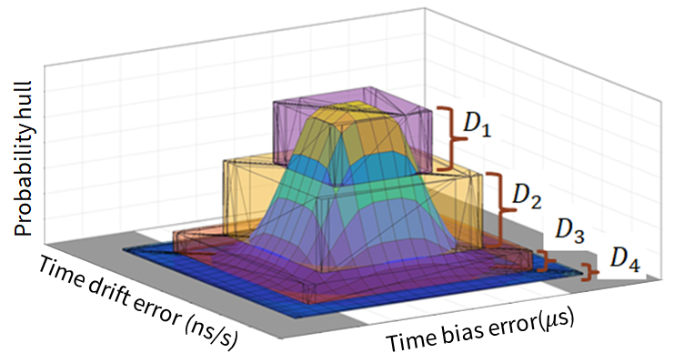

To perform the timing risk analysis, we over-approximate the corrected p-Zonotope by a finite series of polytopes [24]. An example of over-approximation of p-Zonotope by four polytopes to is shown in Fig. 7(a). Thereafter, we compute the intersection area of each th polytope with the unsafe set . Figure 7(b) shows the top-view of over-approximated series of polytopes and an example intersection region of polytope with unsafe set .
The timing risk, seen in Eq. (16), is defined as the sum across polytopes of their intersection area, which is denoted by , with the unsafe set times the max probability of th polytope, which is denoted by . The max probability of th polytope is at its top face and equals the probability of corrected p-Zonotope at that level. For computational tractability, we represent the p-Zonotope by a finite number of polytopes and a -confidence set. The -confidence set [24] thresholds the tail of a p-Zonotope by a pre-defined parameter , such that , where erf denotes the error function [30]. From [24], the probability that the state estimation error lies outside the -confidence set of corrected p-Zonotope is .
| (16) |
3.4 Implementation details
Figure 8 summarizes the implementation steps of the proposed SR-DKF described in Sections 3.1-3.3. We assume that the th receiver is authentic during initialization. Therefore, at iteration , we define the predicted p-Zonotope of the state estimation error to be zero-mean center, with non-zero generator and over-bounding covariance matrices.

4 RESULTS AND ANALYSIS
We validate the robustness of the proposed SR-DKF algorithm to not only mitigate the effect of spoofing but also estimate the secure GPS timing and its associated timing risk across all the receivers in the network. We perform set operations of stochastic reachability and transform across various set representations, such as polytopes, zonotopes, p-Zonotopes, etc., using a publicly-available MATLAB toolbox, known as COntinuous Reachability Analyzer (CORA) [31].
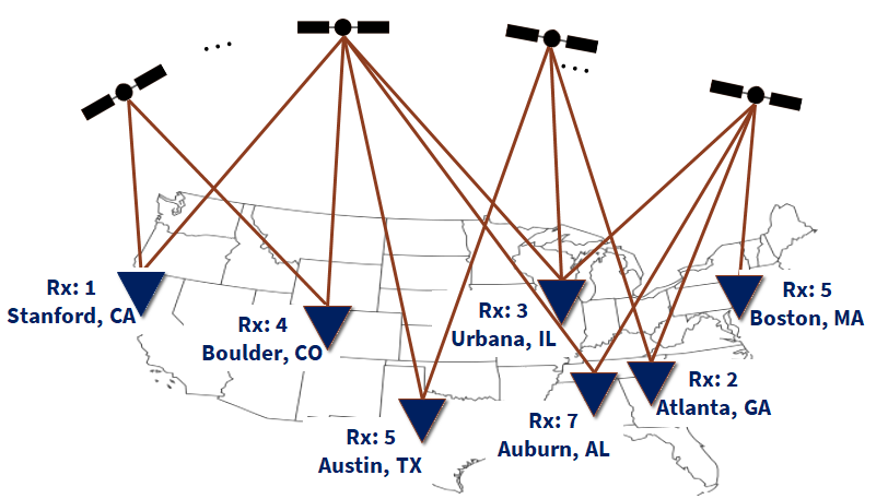
As shown in Fig. 9, we design a simulated network of seven GPS receivers, , that are spatially distributed across the US. The network of GPS receivers indexed from to are located in 1) Stanford, CA; 2) Atlanta, GA; 3) Urbana, IL; 4) Boulder, CO; 5) Austin, TX; 6) Boston, MA; and 7) Auburn, AL. We utilized a C++ language-based software-defined GPS simulator known as GPS-SIM-SDR [32, 33] to simulate the raw GPS signals received at each location in the network. Later, we post-processed the simulated GPS signals using a MATLAB-based software-defined radio known as SoftGNSS [34]. We define the simulated errors observed in the system during authentic conditions to have the following characteristics:
-
1.
For the process noise in GPS time (the first global state ), the mean and covariance of the time-varying Gaussian distribution lies between [s, s] and [s, s], respectively; Similarly, for the process noise in its drift rate (the second global state ), the time-varying mean and covariance lies between [ ns/s, ns/s] and [ ns/s, ns/s], respectively;
-
2.
For the measurement noise in GPS pseudoranges, the mean and covariance of the time-varying Gaussian distribution lies between [s, s] and [s, s], respectively; Similarly, for the measurement noise in GPS Doppler, the time-varying mean and covariance lies between [ ns/s, ns/s] and [ ns/s, ns/s], respectively. We consider all the receivers in this simulated setup to have the same bounds.
-
3.
For the initial state error bounds in GPS time (the first global state ), the mean and covariance of the time-varying Gaussian distribution lies between [s, s] and [s, s], respectively; Similarly, for the initial state error bounds in the second global state , the time-varying mean and covariance lies between [ ns/s, ns/s] and [ ns/s, ns/s], respectively;
As discussed earlier in Fig. 8, we initialize our SR-DKF algorithm by pre-defining the following p-Zonotopes : process noise , measurement noise , and initial state estimation error . We formulate the p-Zonotopes from the above-listed errors bounds in the same manner as the example discussed earlier in Section 2.1.
4.1 During a coordinated signal-level spoofing attack
In the first set of experiments, we consider sparse connectivity among the seven receivers in the network. Figure 10(a) showcases the connectivity matrix where a green tick indicates the presence of a bidirectional communication link while a red cross indicates otherwise. Note that each receiver is connected to itself by default. We induce a simulated coordinated signal-level spoofing attack in the simulated GPS measurements received at two GPS receivers in the network, i.e., , which is located in Stanford, CA and , which is located in Austin, TX. Between the time duration s, the first spoofing attack manipulates the GPS time at to deviate at a rate of ns/s, and the second spoofing attack, which occurs between s, deviates the GPS time of at a rate of ns/s.
In Fig. 10(b), we show the performance of the point-valued state estimation via an adaptive DKF framework, where even the receivers that are not directly spoofed, e.g., , exhibit high state estimation errors. Also, in Fig. 10(c), we show the state estimation accuracy achieved via a point-valued single-receiver-based adaptive KF. In both these point-valued approaches, the measurement noise covariance is adaptively estimated via Eq. (6) by setting the forgetting factor . Based on the maximum error values listed in Table 1, we observe that both the approaches violate the IEEE C37.118.1a-2014 standards. In Fig. 10(d), we validate that our proposed SR-DKF algorithm provides a secure estimate of GPS timing with maximum error of s across all receivers, and thereby complies with the IEEE standards at all times. The quantitative maximum error values of the receiver network for the above-described state estimation approaches are listed in Table 1.


| State estimation approach | ||||||||||
|---|---|---|---|---|---|---|---|---|---|---|
|
8.27 | 7.42 | 6.81 | 6.79 | 8.43 | 7.10 | 7.40 | |||
|
35.88 | 6.47 | 15.24 | 6.70 | 74.68 | 6.26 | 6.36 | |||
| s) |
|
257.36 | 7.36 | 9.48 | 6.43 | 118.90 | 6.46 | 6.48 | ||
|
22.05 | 19.12 | 20.54 | 17.12 | 33.23 | 16.98 | 18.01 | |||
|
80.68 | 23.60 | 39.94 | 19.95 | 125.23 | 18.01 | 20.88 | |||
| (ns/s) |
|
415.39 | 17.90 | 22.75 | 18.71 | 122.94 | 16.21 | 17.04 | ||
In Fig. 11, we plot the attack status of the GPS measurements at each receiver in the network. In accordance with Section 3.2, we demonstrate that the proposed SR-DKF algorithm successfully detects and mitigates spoofing in the GPS measurements of and while accurately categorizing the other receivers, i.e., to be non-spoofed with attack status at all times. We observe that the spoofing attack with higher drift rate is mitigated quicker, i.e., ns/s in , as compared to the one with lower drift rate, i.e., ns/s in .
In Fig. 12, we showcase the timing risk associated with the estimated GPS timing, i.e., the probability of GPS time to violate the IEEE C37.118.1a-2014 standards. This is computed by analyzing the intersection of the corrected p-Zonotope with the unsafe set , as discussed in Section 3.3. An increase or jump in measure of timing risk is based on the adaptive gain matrix that in turn depends on the estimated attack status of the receiver. Therefore, an increase in the timing risk for till s is consistent with the decrease in measurement reliability, which is evident from Fig 11. By comparing Fig. 10(a) and Fig. 12, we observe a direct correlation between the value of timing risk to the number of reliable measurements available for the calculation of corrected p-Zonotope. For instance, since none of the four neighbors of are spoofed, the estimated timing risk is consistently low, i.e., , for the entire experiment duration. In contrast, has significantly high timing risk because two out of its three neighbors are spoofed. Similarly, when only one out of three neighbors at is spoofed, the order of timing risk magnitude is whereas when one out of two neighbors are spoofed at , the timing risk is a higher order magnitude of . Therefore, our SR-DKF estimates a robust measure of the timing risk across all receivers in the network.


4.1.1 Robustness analysis of the proposed SR-DKF algorithm
In the second set of experiments, we demonstrate the robustness of the proposed SR-DKF algorithm as the number of receivers in the neighborhood set is varied. Considering a total experiment duration of s and a network of seven receivers seen in Fig. 9, we induced a simulated meaconing attack between s in the GPS measurements that is received at located at Stanford, CA.
In Fig. 13, we analyzed the variation in the timing risk associated with the estimated GPS time of as the number of receivers in the network is increased. For each size of the receiver network that ranges from to , we consider the presence of a fully-connected bidirectional communication network and perform Monte-Carlo runs for four meaconing magnitudes of s, s, s, and s. We successfully demonstrated that as the number of receivers interacting with the , i.e., , increases, the associated timing risk decreases. Particularly, for , the decrease in timing risk is on the order of and hence, considered insignificant. Similarly, the effect of meaconing magnitude on the timing risk decreases as the number of interacting receivers associated with increases. Therefore, we validated the proposed SR-DKF algorithm that requires only a handful of distributed GPS receivers to achieve robust performance.

5 CONCLUSIONS
In summary, we developed a Stochastic Reachability-based Distributed Kalman Filter (SR-DKF) to perform set-valued state estimation using a network of GPS receivers that estimate not only the point-valued mean but also the stochastic reachable set of state (i.e., GPS time and its drift rate). By parameterizing the stochastic reachable set via probabilistic zonotopes (p-Zonotopes), we derived the time and measurement update steps of the set-valued DKF to estimate the predicted and corrected p-Zonotope of timing error, respectively. To compute secure GPS time for a network of receivers, we designed a two-tiered approach: first, we performed spoofing mitigation at measurement-level via deviation of measurement innovation from its expected stochastic set (represented by the p-Zonotope). Second, we performed timing risk analysis at state-level via intersection probability of corrected p-Zonotope with an unsafe set, i.e., a set that violates the IEEE C37.118.1a-2014 standards. To our knowledge, no prior literature exists on secure state estimation via stochastic reachability nor on timing risk quantification during spoofing.
Under a simulated coordinated signal-level spoofing that affects two among a network of seven sparsely-connected GPS receivers, the proposed SR-DKF algorithm demonstrated a higher timing accuracy, successfully mitigated the spoofing attacks, and estimated a robust measure of timing risk. While our algorithm showed a maximum timing error of only s, both the conventional DKF and single-receiver-based adaptive KF showed high estimation errors that violate the IEEE C37.118.1a-2014 threshold of s. Furthermore, by varying the number of receivers and attack magnitudes, we performed extensive Monte Carlo runs to validate the sensitivity of estimated timing risk.
ACKNOWLEDGEMENTS
We would like to thank Ashwin Kanhere, Siddharth Tanwar, and Tara Yasmin Mina for their help in revising the paper and presentation. We would also like to thank the members of NAVLab research at Stanford University for their thoughtful input on this work and paper.
This material is based upon work supported by the Department of Energy under Award Number DE-OE0000780.
This report was prepared as an account of work sponsored by an agency of the United States Government. Neither the United States Government nor any agency thereof, nor any of their employees, makes any warranty, express or implied, or assumes any legal liability or responsibility for the accuracy, completeness, or usefulness of any information, apparatus, product, or process disclosed, or represents that its use would not infringe privately owned rights. Reference herein to any specific commercial product, process, or service by trade name, trademark, manufacturer, or otherwise does not necessarily constitute or imply its endorsement, recommendation, or favoring by the United States Government or any agency thereof. The views and opinions of authors expressed herein do not necessarily state or reflect those of the United States Government or any agency thereof.
References
- [1] G. Duan, Y. Yan, X. Xie, H. Tao, D. Yang, L. Wang, K. Zhao, and J. Li, “Development status quo and tendency of wide area phasor measuring technology,” Automation of Electric Power Systems, vol. 39, no. 1, pp. 73–80, 2015.
- [2] P. Overholt, D. Ortiz, and A. Silverstein, “Synchrophasor technology and the doe: Exciting opportunities lie ahead in development and deployment,” IEEE Power and Energy Magazine, vol. 13, no. 5, pp. 14–17, 2015.
- [3] J. Taft, “Assessment of existing synchrophasor networks,” Pacific northwest national laboratory (PNNL) technical report. https://gridarchitecture. pnnl. gov/media/whitepapers/Synchrophasor_net_assessment_final. pdf. Accessed April, 2018.
- [4] P. T. Myrda and K. Koellner, “NASPInet - the internet for synchrophasors,” in 2010 43rd Hawaii International Conference on System Sciences, 2010, pp. 1–6.
- [5] L. Heng, D. B. Work, and G. X. Gao, “GPS signal authentication from cooperative peers,” IEEE Transactions on Intelligent Transportation Systems, vol. 16, no. 4, pp. 1794–1805, 2014.
- [6] P. Misra and P. Enge, “Global positioning system: signals, measurements and performance second edition,” Global Positioning System: Signals, Measurements And Performance Second Editions, vol. 206, 2006.
- [7] D. P. Shepard, T. E. Humphreys, and A. A. Fansler, “Evaluation of the vulnerability of phasor measurement units to GPS spoofing attacks,” International Journal of Critical Infrastructure Protection, vol. 5, no. 3-4, pp. 146–153, 2012.
- [8] S. Bhamidipati and G. X. Gao, “GPS multi-receiver joint direct time estimation and spoofer localization,” IEEE Transactions on Aerospace and Electronic Systems, vol. 55, no. 4, pp. 1907–1919, 2018.
- [9] K. E. Martin, “Synchrophasor measurements under the IEEE standard C37. 118.1-2011 with amendment C37. 118.1 a,” IEEE Transactions on Power Delivery, vol. 30, no. 3, pp. 1514–1522, 2015.
- [10] “North american synchrophasor initiative,” [Online] Available: https://www.naspi.org/node/372, (Accessed as of September, 2020).
- [11] D.-Y. Yu, A. Ranganathan, T. Locher, S. Capkun, and D. Basin, “Short paper: Detection of GPS spoofing attacks in power grids,” in Proceedings of the 2014 ACM conference on Security and privacy in wireless & mobile networks, 2014, pp. 99–104.
- [12] A. Khalajmehrabadi, N. Gatsis, D. Akopian, and A. F. Taha, “Real-time rejection and mitigation of time synchronization attacks on the global positioning system,” IEEE Transactions on Industrial Electronics, vol. 65, no. 8, pp. 6425–6435, 2018.
- [13] S. Bhamidipati, T. Y. Mina, and G. X. Gao, “GPS time authentication against spoofing via a network of receivers for power systems,” in 2018 IEEE/ION Position, Location and Navigation Symposium (PLANS). IEEE, 2018, pp. 1485–1491.
- [14] C. Günther, “A survey of spoofing and counter-measures,” NAVIGATION: Journal of The Institute of Navigation, vol. 61, no. 3, pp. 159–177, 2014.
- [15] D. Schmidt, K. Radke, S. Camtepe, E. Foo, and M. Ren, “A survey and analysis of the GNSS spoofing threat and countermeasures,” ACM Computing Surveys (CSUR), vol. 48, no. 4, pp. 1–31, 2016.
- [16] D. Shi, T. Chen, and L. Shi, “On set-valued Kalman filtering and its application to event-based state estimation,” IEEE Transactions on Automatic Control, vol. 60, no. 5, pp. 1275–1290, 2014.
- [17] V. Shiryaev and E. Podivilova, “Set-valued estimation of linear dynamical system state when disturbance is decomposed as a system of functions,” Procedia Engineering, vol. 129, pp. 252–258, 2015.
- [18] P. L. Combettes, “The foundations of set theoretic estimation,” Proceedings of the IEEE, vol. 81, no. 2, pp. 182–208, 1993.
- [19] M. Prandini, J. Hu, C. Cassandras, and J. Lygeros, “Stochastic reachability: Theory and numerical approximation,” Stochastic hybrid systems, Automation and Control Engineering Series, vol. 24, pp. 107–138, 2006.
- [20] S. Bhamidipati and G. X. Gao, “Multiple GPS fault detection and isolation using a graph-SLAM framework,” in 31st International Technical Meeting of the Satellite Division of the Institute of Navigation, ION GNSS+ 2018. Institute of Navigation, 2018, pp. 2672–2681.
- [21] ——, “GPS spoofing mitigation and timing risk analysis in networked PMUs via stochastic reachability,” in 33rd International Technical Meeting of the Satellite Division of the Institute of Navigation, ION GNSS+ 2020. Institute of Navigation (Accepted), 2020.
- [22] S. P. Talebi and S. Werner, “Distributed Kalman filtering: Consensus, diffusion, and mixed,” in 2018 IEEE Conference on Control Technology and Applications (CCTA). IEEE, 2018, pp. 1126–1132.
- [23] A. Alanwar, H. Said, and M. Althoff, “Distributed secure state estimation using diffusion Kalman filters and reachability analysis,” in 2019 IEEE 58th Conference on Decision and Control (CDC). IEEE, 2019, pp. 4133–4139.
- [24] M. Althoff, O. Stursberg, and M. Buss, “Safety assessment for stochastic linear systems using enclosing hulls of probability density functions,” in 2009 European Control Conference (ECC). IEEE, 2009, pp. 625–630.
- [25] J. R. Nuñez, C. R. Anderton, and R. S. Renslow, “Optimizing colormaps with consideration for color vision deficiency to enable accurate interpretation of scientific data,” PloS one, vol. 13, no. 7, p. e0199239, 2018.
- [26] M. Althoff and J. M. Dolan, “Online verification of automated road vehicles using reachability analysis,” IEEE Transactions on Robotics, vol. 30, no. 4, pp. 903–918, 2014.
- [27] E. W. Grafarend, Linear and nonlinear models: fixed effects, random effects, and mixed models. de Gruyter, 2006.
- [28] L. Heng, G. X. Gao, T. Walter, and P. Enge, “GPS signal-in-space anomalies in the last decade: Data mining of 400,000,000 GPS navigation messages,” in 23rd International Technical Meeting of the Satellite Division of the Institute of Navigation 2010, ION GNSS 2010, 2010, pp. 3115–3122.
- [29] S. T. Watt, S. Achanta, H. Abubakari, E. Sagen, Z. Korkmaz, and H. Ahmed, “Understanding and applying precision time protocol,” in 2015 Saudi Arabia Smart Grid (SASG). IEEE, 2015, pp. 1–7.
- [30] K. B. Oldham, J. C. Myland, and J. Spanier, “The error function erf (x) and its complement erfc (x),” in An Atlas of Functions. Springer, 2008, pp. 405–415.
- [31] M. Althoff, “CORA 2016 manual,” TU Munich, vol. 85748, 2016.
- [32] T. Ebinuma, “GPS-SDR-SIM,” [Online] Available: https://github.com/osqzss/gps-sdr-sim, (Accessed as of June, 2020).
- [33] S. Bhamidipati, K. J. Kim, H. Sun, and P. V. Orlik, “GPS spoofing detection and mitigation in PMUs using distributed multiple directional antennas,” in ICC 2019-2019 IEEE International Conference on Communications (ICC). IEEE, 2019, pp. 1–7.
- [34] K. Paul, “Soft GNSS,” [Online] Available: https://github.com/kristianpaul/SoftGNSS, (Accessed as of June, 2020).