This paper was converted on www.awesomepapers.org from LaTeX by an anonymous user.
Want to know more? Visit the Converter page.

11institutetext: J.N. Neuberger 22institutetext: Department of Mathematics, North Carolina State University,
Raleigh, NC.
33institutetext: A. Alexanderian 44institutetext: Department of Mathematics, North Carolina State University,
Raleigh, NC.
55institutetext: B.v.B. Waanders
Center for Computing Research, Sandia National Labs,
Albuquerque, NM.

Goal oriented optimal design of infinite-dimensional Bayesian inverse problems using quadratic approximations

J. Nicholas Neuberger    Alen Alexanderian    Bart van Bloemen Waanders
Abstract

We consider goal-oriented optimal design of experiments for infinite-dimensional Bayesian linear inverse problems governed by partial differential equations (PDEs). Specifically, we seek sensor placements that minimize the posterior variance of a prediction or goal quantity of interest. The goal quantity is assumed to be a nonlinear functional of the inversion parameter. We propose a goal-oriented optimal experimental design (OED) approach that uses a quadratic approximation of the goal-functional to define a goal-oriented design criterion. The proposed criterion, which we call the GqG_{q}-optimality criterion, is obtained by integrating the posterior variance of the quadratic approximation over the set of likely data. Under the assumption of Gaussian prior and noise models, we derive a closed-form expression for this criterion. To guide development of discretization invariant computational methods, the derivations are performed in an infinite-dimensional Hilbert space setting. Subsequently, we propose efficient and accurate computational methods for computing the GqG_{q}-optimality criterion. A greedy approach is used to obtain GqG_{q}-optimal sensor placements. We illustrate the proposed approach for two model inverse problems governed by PDEs. Our numerical results demonstrate the effectiveness of the proposed strategy. In particular, the proposed approach outperforms non-goal-oriented (A-optimal) and linearization-based (c-optimal) approaches.

1 Introduction

Inverse problems are common in science and engineering applications. In such problems, we use a model and data to infer uncertain parameters, henceforth called inversion parameters, that are not directly observable. We consider the case where measurement data are collected at a set of sensors. In practice, often only a few sensors can be deployed. Thus, optimal placement of the sensors is critical. Addressing this requires solving an optimal experimental design (OED) problem AtkinsonDonev92 ; Ucinski05 ; Pukelsheim06 .

In some applications, the estimation of the inversion parameter is merely an intermediate step. For example, consider a source inversion problem in a heat transfer application. In such problems, one is often interested in prediction quantities such as the magnitude of the temperature within a region of interest or heat flux through an interface. A more complex example is a wildfire simulation problem, where one may seek to estimate the source of the fire, but the emphasis is on prediction quantities summarizing future states of the system. In such problems, design of experiments should take the prediction/goal quantities of interest into account. Failing to do so might result in sensor placements that do not result in optimal uncertainty reduction in the prediction/goal quantities. This points to the need for a goal-oriented OED approach. This is the subject of this article.

We focus on Bayesian linear inverse problems governed by PDEs with infinite-dimensional parameters. To make matters concrete, we consider the observation model,

𝒚=m+𝜼.\boldsymbol{y}=\mathcal{F}m+\boldsymbol{\eta}. (1.1)

Here, 𝒚d\boldsymbol{y}\in\mathbb{R}^{d} is a vector of measurement data, \mathcal{F} is a linear parameter-to-observable map, mm is the inversion parameter, and 𝜼\boldsymbol{\eta} is a random variable that models measurement noise. We consider the case where mm belongs to an infinite-dimensional real separable Hilbert space \mathscr{M} and :d\mathcal{F}:\mathscr{M}\to\mathbb{R}^{d} is a continuous linear transformation. The inverse problem seeks to estimate mm using the observation model (1.1). Examples of such problems include source inversion or initial state estimation in linear PDEs. See Section 2, for a brief summary of the requisite background regarding infinite-dimensional Bayesian linear inverse problems and OED for such problems.

We consider the case where solving the inverse problem is an intermediate step and the primary focus is accurate estimation of a scalar-valued prediction quantity characterized by a nonlinear goal-functional,

𝒵:.\mathcal{Z}:\mathscr{M}\to\mathbb{R}. (1.2)

In the present work, we propose a goal-oriented OED approach that seeks to find sensor placements minimizing the posterior uncertainty in such goal-functionals.

Related work. The literature devoted to OED is extensive. Here, we discuss articles that are closely related to the present work. OED for infinite-dimensional Bayesian linear inverse problems has been addressed in several works in the past decade; see e.g., AlexanderianPetraStadlerEtAl14 ; AlexanderianSaibaba18 ; HermanAlexanderianSaibaba20 . Goal-oriented approaches for OED in inverse problems governed by differential equations have appeared in HerzogRiedelUcinski18 ; Li19 ; ButlerJakemanWildey20 . The article HerzogRiedelUcinski18 considers nonlinear problems with nonlinear goal operators. In that article, a goal-oriented OED criterion is obtained using linearization of the goal operator and an approximate (linearization-based) covariance matrix for the inversion parameter. The thesis Li19 considers linear inverse problems with Gaussian prior and noise models, where the goal operator itself is a linear transformation of the inversion parameters. A major focus of that thesis is the study of methods for the combinatorial optimization problem corresponding to optimal sensor placement. The work ButlerJakemanWildey20 considers a stochastic inverse problem formulation, known as data-consistent framework ButlerJakemanWildey18 . This approach, while related, is different from traditional Bayesian inversion. Goal-oriented OED for infinite-dimensional linear inverse problems was studied in AttiaAlexanderianSaibaba18 ; WuChenGhattas23a . These articles consider goal-oriented OED for the case of linear parameter-to-goal mappings.

For the specific class of problems considered in the present work, a traditional approach is to consider a linearization of the goal-functional 𝒵\mathcal{Z} around a nominal parameter m¯\bar{m}. Considering the posterior variance of this linearized functional leads to a specific form of the well-known c-optimality criterion ChalonerVerdinelli95 . However, a linear approximation does not always provide sufficient accuracy in characterizing the uncertainty in the goal-functional. In such cases, a more accurate approximation to 𝒵\mathcal{Z} is desirable.

Our approach and contributions. We consider a quadratic approximation of the goal-functional. Thus, 𝒵\mathcal{Z} is approximated by

𝒵(m)𝒵quad(m):=𝒵(m¯)+𝒵(m¯),mm¯+122𝒵(m¯)(mm¯),mm¯.\mathcal{Z}(m)\approx\mathcal{Z}_{\text{quad}}(m)\vcentcolon=\mathcal{Z}(\bar{m})+\left\langle\nabla\mathcal{Z}(\bar{m}),m-\bar{m}\right\rangle+\frac{1}{2}\left\langle\nabla^{2}\mathcal{Z}(\bar{m})(m-\bar{m}),m-\bar{m}\right\rangle. (1.3)

Following an A-optimal design approach, we consider the posterior variance of the quadratic approximation, 𝕍μpost𝒚{𝒵quad}\mathbb{V}_{\mu_{\text{post}}^{\boldsymbol{y}}}\{\mathcal{Z}_{\text{quad}}\}. We derive an analytic expression for this variance in the infinite-dimensional setting, in Section 3. Note, however, that this variance expression depends on data 𝒚\boldsymbol{y}, which is not available a priori. To overcome this, we compute the expectation of this variance expression with respect to data. This results in a data-averaged design criterion, which we call the GqG_{q}-optimality criterion. Here, GG indicates the goal-oriented nature of the criterion and qq indicates the use of a quadratic approximation. The closed-form analytic expression for this criterion is derived in Theorem 3.2.

Subsequently, in Section 4, we present three computational approaches for fast estimation of Ψ\Psi, relying on Monte Carlo trace estimators, low-rank spectral decompositions, or a low-rank singular value decomposition (SVD) of \mathcal{F}, respectively. Focusing on problems where the goal functional 𝒵\mathcal{Z} is defined in terms of PDEs, our methods rely on adjoint-based expressions for the gradient and Hessian of 𝒵\mathcal{Z}. We demonstrate effectiveness of the proposed goal-oriented approach in a series of computational experiments in Section 5.1 and Section 5.2. The example in Section 5.1 involves inversion of a volume source term in an elliptic PDE with the goal defined as a quadratic functional of the state variable. The example in Section 5.2 concerns a porous medium flow problem with a nonlinear goal functional.

The key contributions of this article are as follows:

  • \bullet

    derivation of a novel goal-oriented design criterion, the GqG_{q}-optimality criterion, based on a quadratic approximation of the goal-functional, in an infinite-dimensional Hilbert space setting (see Section 3);

  • \bullet

    efficient computational methods for estimation of the GqG_{q}-optimality criterion (see Section 4);

  • \bullet

    extensive computational experiments, demonstrating the importance of goal-oriented OED and effectiveness of the proposed approach (see Section 5).

2 Background

In this section, we discuss the requisite background concepts and notations regarding Bayesian linear inverse problems and OED.

2.1 Bayesian linear inverse problems

The key components of a Bayesian inverse problem are the prior distribution, the data-likelihood, and the posterior distribution. The prior encodes our prior knowledge about the inversion parameter, which we denote by mm. The likelihood, which incorporates the parameter-to-observable map, describes the conditional distribution of data for a given inversion parameter. Finally, the posterior is a distribution law for mm that is conditioned on the observed data and is consistent with the prior. These components are related via the Bayes formula Stuart10 . Here, we summarize the process for the case of linear Bayesian inverse problem.

The data likelihood. We consider a bounded linear parameter-to-observable map, :d\mathcal{F}:\mathscr{M}\to\mathbb{R}^{d}. In linear inverse problems governed by PDEs, we define \mathcal{F} as the composition of a linear PDE solution operator 𝒮\mathcal{S} and a linear observation operator \mathcal{B}, which extracts solution values at a prespecified set of measurement points. Hence, =𝒮\mathcal{F}=\mathcal{B}\mathcal{S}. In the present, work, we consider observation models of the form

𝒚=m+𝜼,where𝜼𝖭(0,σ2𝐈).\boldsymbol{y}=\mathcal{F}m+\boldsymbol{\eta},\quad\text{where}\quad\boldsymbol{\eta}\sim\mathsf{N}(0,\sigma^{2}\mathbf{I}). (2.1)

We assume mm and 𝜼\boldsymbol{\eta} are independent, which implies, 𝒚|m𝖭(m,σ2𝐈)\boldsymbol{y}|m\sim\mathsf{N}(\mathcal{F}m,\sigma^{2}\mathbf{I}). This defines the data-likelihood.

Prior. Herein, =L2(Ω)\mathscr{M}=L^{2}(\Omega), where Ω\Omega is a bounded domain in two- or three-space dimensions. This space is equipped with the L2(Ω)L^{2}(\Omega) inner product ,\left\langle\cdot,\cdot\right\rangle and norm =,1/2\|\cdot\|=\left\langle\cdot,\cdot\right\rangle^{1/2}. We consider a Gaussian prior law μpr:=𝖭(mpr,𝒞pr)\mu_{\text{pr}}:=\mathsf{N}(m_{\text{pr}},\mathcal{C}_{\text{pr}}). To define the prior, we follow the approach in Stuart10 ; Bui-ThanhGhattasMartinEtAl13 . The prior mean is assumed to be a sufficiently regular element of \mathscr{M} and the prior covariance operator 𝒞pr\mathcal{C}_{\text{pr}} is defined as the inverse of a differential operator. Specifically, let \mathcal{E} be the mapping sms\mapsto m, defined by the solution operator of

a1(a2Δm+m)\displaystyle-a_{1}(a_{2}\Delta m+m) =sin Ω,\displaystyle=s\quad\text{in }\Omega, (2.2)
m𝒏\displaystyle\nabla m\cdot\boldsymbol{n} =0,on Ω,\displaystyle=0,\quad\text{on }\partial\Omega,

where a1a_{1} and a2a_{2} are positive constants. Then, the prior covariance is defined as 𝒞pr:=2\mathcal{C}_{\text{pr}}:=\mathcal{E}^{2}.

Posterior. For a Bayesian linear inverse problem with a Gaussian prior and a Gaussian noise model given by (2.1), it is well-known Stuart10 that the posterior is the Gaussian measure μpost𝒚:=𝖭(mMAP𝒚,𝒞post)\mu_{\text{post}}^{\boldsymbol{y}}\vcentcolon=\mathsf{N}\left(m_{\text{MAP}}^{\boldsymbol{y}},\mathcal{C}_{\text{post}}\right) with

𝒞post=(σ2+𝒞pr1)1andmMAP𝒚=𝒞post(σ2𝒚+𝒞pr1mpr),\mathcal{C}_{\text{post}}=\left(\sigma^{-2}\mathcal{F}^{*}\mathcal{F}+\mathcal{C}_{\text{pr}}^{-1}\right)^{-1}\quad\text{and}\quad m_{\text{MAP}}^{\boldsymbol{y}}=\mathcal{C}_{\text{post}}\left(\sigma^{-2}\mathcal{F}^{*}\boldsymbol{y}+\mathcal{C}_{\text{pr}}^{-1}m_{\text{pr}}\right), (2.3)

where \mathcal{F}^{*} denotes the adjoint of \mathcal{F}. Here, the posterior mean is the maximum a posteriori probability (MAP) point. Also, recall the variational characterization of this MAP point as the unique global minimizer of

J(m):=12σ2m𝒚22+12mmpr𝒞pr12J(m)\vcentcolon=\frac{1}{2\sigma^{2}}\|\mathcal{F}m-\boldsymbol{y}\|^{2}_{2}+\frac{1}{2}\|m-m_{\text{pr}}\|_{\mathcal{C}_{\text{pr}}^{-1}}^{2} (2.4)

in the Cameron–Martin space, range(𝒞pr1/2)\mathrm{range}(\mathcal{C}_{\text{pr}}^{1/2}); see DashtiStuart17 . The Cameron–Martin space plays a key role in the study of Gaussian measures on Hilbert spaces. In particular, this space is important in the theory of Bayesian inverse problems with Gaussian priors. Here, 𝒞pr12\|\cdot\|_{\mathcal{C}_{\text{pr}}^{-1}}^{2} is the Cameron–Martin norm, m𝒞pr12=𝒞pr1/2m2\|m\|_{\mathcal{C}_{\text{pr}}^{-1}}^{2}=\|\mathcal{C}_{\text{pr}}^{-1/2}m\|^{2}.

It can be shown that the Hessian of JJ, denoted by \mathcal{H}, satisfies =𝒞post1\mathcal{H}=\mathcal{C}_{\text{post}}^{-1}. In what follows, the Hessian of data-misfit term in (2.4) will be important. We denote this Hessian by mis:=σ2\mathcal{H}_{\text{mis}}\vcentcolon=\sigma^{-2}\mathcal{F}^{*}\mathcal{F}. A closely related operator is the prior-preconditioned data-misfit Hessian,

~mis:=𝒞pr1/2mis𝒞pr1/2,\tilde{\mathcal{H}}_{\text{mis}}\vcentcolon=\mathcal{C}_{\text{pr}}^{1/2}\mathcal{H}_{\text{mis}}\mathcal{C}_{\text{pr}}^{1/2}, (2.5)

which also plays a key role in the discussions that follow.

Lastly, we remark on the case when the forward operator is affine. This will be the case for inverse problems governed by linear PDEs with inhomogeneous source volume or boundary source terms. The model inverse problem considered in Section 5.2 is an example of such problems. In that case, the forward operator may be represented as the affine map 𝒢(m)=m+𝒅\mathcal{G}(m)=\mathcal{F}m+\boldsymbol{d}, where \mathcal{F} is a bounded linear transformation. Under the Gaussian assumption on the prior and noise, the posterior is a Gaussian with the same covariance operator as in (2.3) and with the mean given by mMAP𝒚=𝒞post(σ2(𝒚d)+𝒞pr1mpr)m_{\text{MAP}}^{\boldsymbol{y}}=\mathcal{C}_{\text{post}}\left(\sigma^{-2}\mathcal{F}^{*}(\boldsymbol{y}-d)+\mathcal{C}_{\text{pr}}^{-1}m_{\text{pr}}\right).

Discretization. We discretize the inverse problem using the continuous Galerkin finite element method. Consider a nodal finite element basis of compactly supported functions {ϕi}i=1N\{\phi_{i}\}_{i=1}^{N}. The discretized inversion parameter is represented as mh=i=1Nmiϕim_{h}=\sum_{i=1}^{N}m_{i}\phi_{i}. Following common practice, we identify mhm_{h} with the vector of its finite element coefficients, 𝒎=[m1m2mN]\boldsymbol{m}=[m_{1}\;m_{2}\;\cdots\;m_{N}]^{\top}. The discretized inversion parameter space is thus N\mathbb{R}^{N} equipped with the mass-weighted inner product 𝒖,𝒗𝐌:=𝒖𝐌𝒗\left\langle\boldsymbol{u},\boldsymbol{v}\right\rangle_{\mathbf{M}}\vcentcolon=\boldsymbol{u}^{\top}\mathbf{M}\boldsymbol{v}. Here, 𝐌\mathbf{M} is the finite element mass matrix, Mij:=Ωϕi,ϕjd𝒙M_{ij}:=\int_{\Omega}\phi_{i},\phi_{j}\,d\boldsymbol{x}, for i,j{1,,N}i,j\in\{1,\ldots,N\}. Note that this mass-weighted inner product is the discretized L2(Ω)L^{2}(\Omega) inner product. Throughout the article, we use the notation 𝐌N\mathbb{R}^{N}_{\mathbf{M}} for N\mathbb{R}^{N} equipped with the mass-weighted inner product ,𝐌\left\langle\cdot,\cdot\right\rangle_{\mathbf{M}}.

We use boldfaced symbols to represent the discretized versions of the operators appearing in the Bayesian inverse problem formulation. For details on obtaining such discretized operators, see Bui-ThanhGhattasMartinEtAl13 . The discretized solution, observation, and forward operators are denoted by 𝐒\mathbf{S}, 𝐁\mathbf{B}, and 𝐅\mathbf{F}, respectively. Similarly, the discretized Hessian is presented as 𝐇\mathbf{H}. We denote the discretized prior and posterior covariance operators by 𝚪pr\mathbf{\Gamma}_{\text{pr}} and 𝚪post\mathbf{\Gamma}_{\text{post}}, respectively. Note that 𝚪pr\mathbf{\Gamma}_{\text{pr}} and 𝚪post\mathbf{\Gamma}_{\text{post}} are selfadjoint operators on 𝐌N\mathbb{R}^{N}_{\mathbf{M}}.

2.2 Classical optimal experimental design

In the present work, an experimental design corresponds to an array of sensors selected from a set of candidate sensor locations, {xi}i=1nΩ\{x_{i}\}_{i=1}^{n}\subset\Omega. In a classical OED problem, an experimental design is called optimal if it minimizes a notion of posterior uncertainty in the inversion parameter. This is different from a goal-oriented approach, where we seek designs that minimize the uncertainty in a goal quantity of interest.

To formulate an OED problem, it is helpful to parameterize sensor placements in some manner. A common approach is to assign weights to each sensor in the candidate sensor grid. That is, we assign a weight wi0w_{i}\geq 0 to each xix_{i}, i{1,,n}i\in\{1,\ldots,n\}. This way, a sensor placement is identified with a vector 𝒘n\boldsymbol{w}\in\mathbb{R}^{n}. Each wiw_{i} may be restricted to some subset of \mathbb{R} depending on the optimization scheme. Here, we assume wi{0,1}w_{i}\in\{0,1\}; a weight of zero means the corresponding sensor is inactive.

The vector 𝒘\boldsymbol{w} of the design weights is incorporated in the Bayesian inverse problem formulation through the data-likelihood Alexanderian21 . This yields a 𝒘\boldsymbol{w}-dependent posterior measure. In particular, the posterior covariance operator is given by

𝒞post(𝒘)=(𝐖σ+𝒞pr1)1with𝐖σ=σ2diag(𝒘).\mathcal{C}_{\text{post}}(\boldsymbol{w})=\left(\mathcal{F}^{*}\mathbf{W}_{\!\sigma}\mathcal{F}+\mathcal{C}_{\text{pr}}^{-1}\right)^{-1}\quad\text{with}\quad\mathbf{W}_{\!\sigma}=\sigma^{-2}\text{diag}(\boldsymbol{w}). (2.6)

There are several classical criteria in the OED literature. One example is the A-optimality criterion, which is defined as the trace of 𝒞post(𝒘)\mathcal{C}_{\text{post}}(\boldsymbol{w}). The corresponding discretized criterion is

𝚯(𝒘)=tr(𝚪post(𝒘))with𝚪post(𝒘):=(𝐅𝐖σ𝐅+𝚪pr1)1.\mathbf{\Theta}(\boldsymbol{w})=\mathrm{tr}\left(\mathbf{\Gamma}_{\text{post}}(\boldsymbol{w})\right)\quad\text{with}\quad\mathbf{\Gamma}_{\text{post}}(\boldsymbol{w})\vcentcolon=\left(\mathbf{F}^{*}\mathbf{W}_{\!\sigma}\mathbf{F}+\mathbf{\Gamma}_{\text{pr}}^{-1}\right)^{-1}. (2.7)

The A-optimality criterion quantifies the average posterior variance of the inversion parameter field. To define a goal-oriented analogue of the A-optimality criterion, we need to consider the posterior variance of the goal-functional 𝒵\mathcal{Z} in (1.2). This is discussed in the next section.

3 Goal-oriented OED

In a goal-oriented OED problem, we seek designs that minimize the uncertainty in a goal quantity of interest, which is a function of the inversion parameter mm. Here, we consider a nonlinear goal-functional

𝒵:.\mathcal{Z}:\mathscr{M}\to\mathbb{R}. (3.1)

In our target applications, evaluating 𝒵\mathcal{Z} involves solving PDEs. Thus, computing the posterior variance of 𝒵\mathcal{Z} via sampling can be challenging—a potentially large number of samples might be required. Also, computing an optimal design requires evaluation of the design criterion in every step of an optimization algorithm. Furthermore, generating samples from the posterior requires forward and adjoint PDE solves. Thus, design criteria that require sampling 𝒵\mathcal{Z} at every step of an optimization algorithm will be computationally inefficient. One approach to developing a computationally tractable goal-oriented OED approach is to replace 𝒵\mathcal{Z} by a suitable approximation. This leads to the definition of approximate measures of uncertainty in 𝒵\mathcal{Z}.

We can use local approximations of 𝒵\mathcal{Z} to derive goal-oriented criteria. This requires an expansion point, which we denote as m¯\bar{m}\in\mathscr{M}. A simple choice is to let m¯\bar{m} be the prior mean. Another approach, which might be feasible in some applications, is to assume some initial measurement data is available. This data may be used to compute an initial parameter estimate. Such an initial estimate might not be suitable for prediction purposes, but can be used in place of m¯\bar{m}. The matter of expansion point selection is discussed later in Section 5. For now, m¯\bar{m} is considered to be a fixed element in \mathscr{M}. In what follows, we assume 𝒵\mathcal{Z} is twice differentiable and denote

g¯𝒵:=𝒵(m¯)and¯𝒵:=2𝒵(m¯).\bar{g}_{\scriptscriptstyle{\mathcal{Z}}}:=\nabla\mathcal{Z}(\bar{m})\quad\text{and}\quad\bar{\mathcal{H}}_{\scriptscriptstyle{\mathcal{Z}}}:=\nabla^{2}\mathcal{Z}(\bar{m}). (3.2)

A known approach for obtaining an approximate measure of uncertainty in 𝒵(m)\mathcal{Z}(m) is to consider a linearization of 𝒵\mathcal{Z} and compute the posterior variance of this linearization. In the present work, this is referred to as the GG_{\ell}-optimality criterion, denoted by Ψ\Psi^{\ell}. The GG is used to indicate goal, and \ell is a reference to linearization. As seen shortly, this GG_{\ell}-optimality criterion is a specific instance of the Bayesian c-optimality criterion ChalonerVerdinelli95 . Consider the linear approximation of 𝒵\mathcal{Z} given by

𝒵(m)𝒵lin(m):=𝒵(m¯)+g¯𝒵,mm¯.\mathcal{Z}(m)\approx\mathcal{Z}_{\text{lin}}(m)\vcentcolon=\mathcal{Z}(\bar{m})+\left\langle\bar{g}_{\scriptscriptstyle{\mathcal{Z}}},m-\bar{m}\right\rangle. (3.3)

The GG_{\ell}-optimality criterion is

Ψ:=𝕍μpost{𝒵lin}.\Psi^{\ell}\vcentcolon=\mathbb{V}_{\mu_{\text{post}}}\left\{\mathcal{Z}_{\text{lin}}\right\}. (3.4)

It is straightforward to note that

Ψ=𝕍μpost{g¯𝒵,mm¯}=g¯𝒵,mm¯2μpost(dm)=𝒞postg¯𝒵,g¯𝒵,\Psi^{\ell}=\mathbb{V}_{\mu_{\text{post}}}\left\{\left\langle\bar{g}_{\scriptscriptstyle{\mathcal{Z}}},m-\bar{m}\right\rangle\right\}=\int_{\mathscr{M}}\left\langle\bar{g}_{\scriptscriptstyle{\mathcal{Z}}},m-\bar{m}\right\rangle^{2}\,\mu_{\text{post}}(dm)=\left\langle\mathcal{C}_{\text{post}}\bar{g}_{\scriptscriptstyle{\mathcal{Z}}},\bar{g}_{\scriptscriptstyle{\mathcal{Z}}}\right\rangle, (3.5)

where we have used the definition of covariance operator; see (A.1). Letting c=g¯𝒵c=\bar{g}_{\scriptscriptstyle{\mathcal{Z}}}, we obtain the c-optimality criterion 𝒞postc,c\left\langle\mathcal{C}_{\text{post}}c,c\right\rangle. The variance of the linearized goal is an intuitive and tractable choice for a goal-oriented criterion. However, a linearization might severely underestimate the posterior uncertainty in 𝒵\mathcal{Z} or be overly sensitive to choice of m¯\bar{m}.

In the present work, we define an OED criterion based on the quadratic Taylor expansion of 𝒵\mathcal{Z}. This leads to the GqG_{q}-optimality criterion mentioned in the introduction. Consider the quadratic approximation,

𝒵(m)𝒵quad(m):=𝒵(m¯)+g¯𝒵,mm¯+12¯𝒵(mm¯),mm¯.\mathcal{Z}(m)\approx\mathcal{Z}_{\text{quad}}(m)\vcentcolon=\mathcal{Z}(\bar{m})+\left\langle\bar{g}_{\scriptscriptstyle{\mathcal{Z}}},m-\bar{m}\right\rangle+\frac{1}{2}\left\langle\bar{\mathcal{H}}_{\scriptscriptstyle{\mathcal{Z}}}(m-\bar{m}),m-\bar{m}\right\rangle. (3.6)

We can compute 𝕍μpost{𝒵quad}\mathbb{V}_{\mu_{\text{post}}}\left\{\mathcal{Z}_{\text{quad}}\right\} analytically. This is facilitated by Theorem 3.1 below. The result is well-known in the finite-dimensional setting. In the infinite-dimensional setting, this can be obtained from properties of Gaussian measures on Hilbert spaces, some developments in DaPratoZabczyk02 (cf. Remark 1.2.9., in particular), along with the formula for the expected value of a quadratic form on a Hilbert space AlexanderianGhattasEtAl16 . This approach was used in AlexanderianPetraStadlerEtAl17 to derive the expression for the variance of a second order Taylor expansion, within the context of optimization under uncertainty. However, to our knowledge a direct and standalone proof of Theorem 3.1, which is of independent and of broader interest, does not seem to be available in the literature. Thus, we present a detailed proof of this result in the appendix for completeness.

Theorem 3.1 (Variance of a quadratic functional)

Let 𝒜\mathcal{A} be a bounded selfadjoint linear operator on a Hilbert space \mathscr{M} and let bb\in\mathscr{M}. Consider the quadratic functional 𝒵:\mathcal{Z}:\mathscr{M}\to\mathbb{R} given by

𝒵(m):=12𝒜m,m+b,m,m.\mathcal{Z}(m)\vcentcolon=\frac{1}{2}\left\langle\mathcal{A}m,m\right\rangle+\left\langle b,m\right\rangle,\quad m\in\mathscr{M}. (3.7)

Let μ=𝖭(m0,𝒞)\mu=\mathsf{N}(m_{0},\mathcal{C}) be a Gaussian measure on \mathscr{M}. Then, we have

𝕍μ{𝒵}=𝒜m0+b𝒞2+12tr((𝒞𝒜)2).\mathbb{V}_{\mu}\left\{\mathcal{Z}\right\}=\|\mathcal{A}m_{0}+b\|_{\mathcal{C}}^{2}+\frac{1}{2}\mathrm{tr}\big{(}(\mathcal{C}\mathcal{A})^{2}\big{)}.
Proof

See Appendix A. \square

We next consider the posterior variance 𝕍μpost𝒚{𝒵quad}\mathbb{V}_{\mu_{\text{post}}^{\boldsymbol{y}}}\left\{\mathcal{Z}_{\text{quad}}\right\} of 𝒵quad\mathcal{Z}_{\text{quad}}. Using Theorem 3.1, we obtain

𝕍μpost𝒚{𝒵quad}=¯𝒵mMAP𝒚+b𝒞post2+12tr((𝒞post¯𝒵)2),whereb=g¯𝒵¯𝒵m¯.\mathbb{V}_{\mu_{\text{post}}^{\boldsymbol{y}}}\left\{\mathcal{Z}_{\text{quad}}\right\}=\left\|\bar{\mathcal{H}}_{\scriptscriptstyle{\mathcal{Z}}}m_{\text{MAP}}^{\boldsymbol{y}}+b\right\|_{\mathcal{C}_{\text{post}}}^{2}+\frac{1}{2}\mathrm{tr}\big{(}(\mathcal{C}_{\text{post}}\bar{\mathcal{H}}_{\scriptscriptstyle{\mathcal{Z}}})^{2}\big{)},\quad\text{where}\,b=\bar{g}_{\scriptscriptstyle{\mathcal{Z}}}-\bar{\mathcal{H}}_{\scriptscriptstyle{\mathcal{Z}}}\bar{m}. (3.8)

Note that this variance expression depends on data 𝒚\boldsymbol{y}, which is not available when solving the OED problem. Indeed, the main point of solving an OED problem is to determine how data should be collected. Hence, we consider the “data-averaged” criterion,

Ψ:=𝔼μpr{𝔼𝒚|m{𝕍μpost𝒚{𝒵quad}}}.\Psi:=\mathbb{E}_{\mu_{\text{pr}}}\Big{\{}\mathbb{E}_{\boldsymbol{y}|m}\big{\{}\mathbb{V}_{\mu_{\text{post}}^{\boldsymbol{y}}}\{\mathcal{Z}_{\text{quad}}\}\big{\}}\Big{\}}. (3.9)

Here, 𝔼μpr\mathbb{E}_{\mu_{\text{pr}}} and 𝔼𝒚|m\mathbb{E}_{\boldsymbol{y}|m} represent expectations with respect to the prior and likelihood, respectively. This uses the information available in the Bayesian inverse problem formulation to compute the expected value of 𝕍μpost{𝒵quad(m)}\mathbb{V}_{\mu_{\text{post}}}\left\{\mathcal{Z}_{\text{quad}}(m)\right\} over the set of likely data. In the general case of nonlinear inverse problems, such averaged criteria are computed via sample averaging AlexanderianPetraStadlerEtAl16 ; Alexanderian21 . However, in the present setting, exploiting the linearity of the parameter-to-observable map and the Gaussian assumption on prior and noise models, we can compute Ψ\Psi analytically. This is the main result of this section and presented in the following theorem.

Theorem 3.2 (Goal-oriented criterion)

Let Ψ\Psi be as defined in (3.9). Then,

Ψ=¯𝒵(mprm¯)+g¯𝒵𝒞post2+tr(𝒞pr¯𝒵𝒞post¯𝒵)12tr((𝒞post¯𝒵)2).\Psi=\|\bar{\mathcal{H}}_{\scriptscriptstyle{\mathcal{Z}}}(m_{\text{pr}}-\bar{m})+\bar{g}_{\scriptscriptstyle{\mathcal{Z}}}\|_{\mathcal{C}_{\text{post}}}^{2}+\mathrm{tr}\left(\mathcal{C}_{\text{pr}}\bar{\mathcal{H}}_{\scriptscriptstyle{\mathcal{Z}}}\mathcal{C}_{\text{post}}\bar{\mathcal{H}}_{\scriptscriptstyle{\mathcal{Z}}}\right)-\frac{1}{2}\mathrm{tr}\big{(}(\mathcal{C}_{\text{post}}\bar{\mathcal{H}}_{\scriptscriptstyle{\mathcal{Z}}})^{2}\big{)}. (3.10)
Proof

See Appendix B. \square

We call Ψ\Psi in (3.10) the GqG_{q}-optimality criterion. Proving Theorem 3.2 involves three main steps. In the first step, the variance of the quadratic approximation of 𝒵\mathcal{Z} is calculated using Theorem 3.1. This results in (3.8). In the second step, we need to compute the nested expectations in (3.9). Calculating these moments requires obtaining the expectations of linear and quadratic forms with respect to the data-likelihood and prior laws. The derivations rely on facts about measures on Hilbert spaces. Subsequently, using properties of traces of Hilbert space operators, the definitions of the constructs in the inverse problem formulation, and some detailed manipulations, we derive (3.10). See Appendix B, for details.

4 Computational Methods

Computing the GqG_{q}-optimality criterion (3.10) requires computing traces of high-dimensional and expensive to apply operators, which is a computational challenge. To establish a flexible computational framework, in this section, we present three different algorithms for fast estimation of the GqG_{q}-optimality criterion. In Section 4.1, we present an approach based on randomized trace estimators. Then, we present an algorithm that uses the low-rank spectral decomposition of the prior-preconditioned data misfit Hessian in Section 4.2. Finally, in Section 4.3, we present an approach that uses the low-rank SVD of the prior-preconditioned forward operator. In each case, we rely on structure exploiting methods to obtain scalable algorithms.

Before presenting these methods, we briefly discuss the discretization of the GqG_{q}-optimality criterion. In addition to the discretized operators presented in Section 2.1, we require access to the discretized goal functional, denoted as ZZ, and its derivatives. In what follows, we denote

𝒈¯z:=Z(𝒎¯),𝐇¯z:=2Z(𝒎¯),and𝒃¯z:=𝐇¯z(𝒎pr𝒎¯)+𝒈¯z.\bar{\boldsymbol{g}}_{\text{z}}\vcentcolon=\nabla Z(\boldsymbol{\bar{m}}),\quad\bar{\mathbf{H}}_{\text{z}}\vcentcolon=\nabla^{2}Z(\boldsymbol{\bar{m}}),\quad\text{and}\quad\bar{\boldsymbol{b}}_{\text{z}}\vcentcolon=\bar{\mathbf{H}}_{\text{z}}(\boldsymbol{m}_{\text{pr}}-\bar{\boldsymbol{m}})+\bar{\boldsymbol{g}}_{\text{z}}. (4.1)

The discretized GqG_{q}-optimality criterion is given by

𝚿(𝒘)=𝚪post(𝒘)𝒃¯z,𝒃¯z𝐌+tr(𝚪pr𝐇¯z𝚪post(𝒘)𝐇¯z)12tr((𝚪post(𝒘)𝐇¯z)2).\mathbf{\Psi}(\boldsymbol{w})=\left\langle\mathbf{\Gamma}_{\text{post}}(\boldsymbol{w})\bar{\boldsymbol{b}}_{\text{z}},\bar{\boldsymbol{b}}_{\text{z}}\right\rangle_{\mathbf{M}}+\mathrm{tr}\!\left(\mathbf{\Gamma}_{\text{pr}}\bar{\mathbf{H}}_{\text{z}}\mathbf{\Gamma}_{\text{post}}(\boldsymbol{w})\bar{\mathbf{H}}_{\text{z}}\right)-\frac{1}{2}\mathrm{tr}\big{(}(\mathbf{\Gamma}_{\text{post}}(\boldsymbol{w})\bar{\mathbf{H}}_{\text{z}})^{2}\big{)}. (4.2)

Similarly, discretizing the GG_{\ell}-optimality criterion Ψ\Psi^{\ell}, presented in (3.4), yields

𝚿(𝒘)=𝚪post(𝒘)𝒈¯z,𝒈¯z𝐌.\mathbf{\Psi}^{\ell}(\boldsymbol{w})=\left\langle\mathbf{\Gamma}_{\text{post}}(\boldsymbol{w})\bar{\boldsymbol{g}}_{\text{z}},\bar{\boldsymbol{g}}_{\text{z}}\right\rangle_{\mathbf{M}}. (4.3)

4.1 A randomized algorithm

In large-scale inverse problems, it is expensive to build the forward operator, the prior and posterior covariance operators, or the Hessian of the goal-functional, 𝐇¯z\bar{\mathbf{H}}_{\text{z}} in (4.1). Therefore, matrix-free methods that only require applications of these operators on vectors are essential. A key challenge here is computation of the traces in (4.2). In this section, we present an approach for computing 𝚿\mathbf{\Psi} that relies on randomized trace estimation Avron2011 . As noted in AlexanderianPetraStadlerEtAl14 , the trace of a linear operator 𝐓\mathbf{T} on 𝐌N\mathbb{R}^{N}_{\mathbf{M}} can be approximated via

tr(𝐓)1pj=1p𝐓𝝃j,𝝃j𝐌,with𝝃j𝖭(𝟎,𝐌1).\mathrm{tr}\left(\mathbf{T}\right)\approx\frac{1}{p}\sum_{j=1}^{p}\left\langle\mathbf{T}\boldsymbol{\xi}_{j},\boldsymbol{\xi}_{j}\right\rangle_{\mathbf{M}},\quad\text{with}\ \boldsymbol{\xi}_{j}\sim\mathsf{N}(\boldsymbol{0},\mathbf{M}^{-1}). (4.4)

This is known as a Monte Carlo trace estimator. The number pp of the required trace estimator vectors is problem-dependent. However, in practice, often a modest pp (in order of tens) is sufficient for the purpose of optimization.

We use Monte Carlo estimators to approximate the trace terms in (4.2). In particular, we use

tr(𝚪pr𝐇¯z𝚪post𝐇¯z)12tr((𝚪post𝐇¯z)2)=tr((𝚪pr12𝚪post)𝐇¯z𝚪post𝐇¯z)1pj=1p(𝚪pr12𝚪post)𝐇¯z𝚪post𝐇¯z𝝃i,𝝃i𝐌=1pj=1p(𝚪pr12𝚪post)𝝃i,𝐇¯z𝚪post𝐇¯z𝝃i𝐌,\mathrm{tr}\left(\mathbf{\Gamma}_{\text{pr}}\bar{\mathbf{H}}_{\text{z}}\mathbf{\Gamma}_{\text{post}}\bar{\mathbf{H}}_{\text{z}}\right)-\frac{1}{2}\mathrm{tr}\big{(}(\mathbf{\Gamma}_{\text{post}}\bar{\mathbf{H}}_{\text{z}})^{2}\big{)}=\mathrm{tr}\big{(}(\mathbf{\Gamma}_{\text{pr}}-\frac{1}{2}\mathbf{\Gamma}_{\text{post}})\bar{\mathbf{H}}_{\text{z}}\mathbf{\Gamma}_{\text{post}}\bar{\mathbf{H}}_{\text{z}}\big{)}\\ \approx\frac{1}{p}\sum_{j=1}^{p}\left\langle(\mathbf{\Gamma}_{\text{pr}}-\frac{1}{2}\mathbf{\Gamma}_{\text{post}})\bar{\mathbf{H}}_{\text{z}}\mathbf{\Gamma}_{\text{post}}\bar{\mathbf{H}}_{\text{z}}\boldsymbol{\xi}_{i},\boldsymbol{\xi}_{i}\right\rangle_{\mathbf{M}}=\frac{1}{p}\sum_{j=1}^{p}\left\langle(\mathbf{\Gamma}_{\text{pr}}-\frac{1}{2}\mathbf{\Gamma}_{\text{post}})\boldsymbol{\xi}_{i},\bar{\mathbf{H}}_{\text{z}}\mathbf{\Gamma}_{\text{post}}\bar{\mathbf{H}}_{\text{z}}\boldsymbol{\xi}_{i}\right\rangle_{\mathbf{M}},

where we have exploited the fact that 𝚪pr\mathbf{\Gamma}_{\text{pr}} and 𝚪post\mathbf{\Gamma}_{\text{post}} are selfadjoint with respect to the mass-weighted inner product ,𝐌\left\langle\cdot,\cdot\right\rangle_{\mathbf{M}}. Thus, letting

Tp:=1pj=1p(𝚪pr12𝚪post)𝝃i,𝐇¯z𝚪post𝐇¯z𝝃i𝐌,T_{p}\vcentcolon=\frac{1}{p}\sum_{j=1}^{p}\left\langle(\mathbf{\Gamma}_{\text{pr}}-\frac{1}{2}\mathbf{\Gamma}_{\text{post}})\boldsymbol{\xi}_{i},\bar{\mathbf{H}}_{\text{z}}\mathbf{\Gamma}_{\text{post}}\bar{\mathbf{H}}_{\text{z}}\boldsymbol{\xi}_{i}\right\rangle_{\mathbf{M}},

we can estimate 𝚿\mathbf{\Psi} by

𝚿𝚿rand,p:=𝚪post𝒃¯z,𝒃¯z𝐌+Tp.\mathbf{\Psi}\approx\mathbf{\Psi}_{\text{rand,p}}\vcentcolon=\left\langle\mathbf{\Gamma}_{\text{post}}\bar{\boldsymbol{b}}_{\text{z}},\bar{\boldsymbol{b}}_{\text{z}}\right\rangle_{\mathbf{M}}+T_{p}. (4.5)

This enables a computationally tractable approach for approximating 𝚿\mathbf{\Psi}. We outline the procedure for computing 𝚿rand,p\mathbf{\mathbf{\Psi}_{\text{rand,p}}} in Algorithm 1. The computational cost of this approach is discussed in Section 4.4.

The utility of methods based on Monte Carlo trace estimators in the context of OED for large-scale inverse problems has been demonstrated in previous studies such as HaberHoreshTenorio08 ; HaberMagnantLuceroEtAl12 ; AlexanderianPetraStadlerEtAl14 . A key advantage of the present approach is its simplicity. However, further accuracy and efficiency can be attained by exploiting the low-rank structures embedded in the inverse problem. This is discussed in the next section.

Algorithm 1 Algorithm for estimating 𝚿rand,p\mathbf{\mathbf{\Psi}_{\text{rand,p}}}.
1:  Input: {𝝃i}j=1p\{\boldsymbol{\xi}_{i}\}_{j=1}^{p}, 𝚪post\mathbf{\Gamma}_{\text{post}}
2:  Output: 𝚿rand,p\mathbf{\mathbf{\Psi}_{\text{rand,p}}}
3:  Compute 𝒃¯z=𝐇¯z(𝒎pr𝒎¯)+𝒈¯z\bar{\boldsymbol{b}}_{\text{z}}=\bar{\mathbf{H}}_{\text{z}}(\boldsymbol{m_{\text{pr}}}-\boldsymbol{\bar{m}})+\bar{\boldsymbol{g}}_{\text{z}}
4:  Compute 𝒔=𝚪post𝒃¯z\boldsymbol{s}=\mathbf{\Gamma}_{\text{post}}\bar{\boldsymbol{b}}_{\text{z}}
5:  Set T=0T=0
6:  for j=1j=1 to pp do
7:     Compute 𝒕1=(𝐇¯z𝚪post𝐇¯z)𝝃j\boldsymbol{t}_{1}=(\bar{\mathbf{H}}_{\text{z}}\mathbf{\Gamma}_{\text{post}}\bar{\mathbf{H}}_{\text{z}})\boldsymbol{\xi}_{j}
8:     Compute 𝒕2=(𝚪pr12𝚪post)𝝃j\boldsymbol{t}_{2}=(\mathbf{\Gamma}_{\text{pr}}-\frac{1}{2}\mathbf{\Gamma}_{\text{post}})\boldsymbol{\xi}_{j}
9:     Set T=T+𝒕1,𝒕2𝐌T=T+\left\langle\boldsymbol{t}_{1},\boldsymbol{t}_{2}\right\rangle_{\mathbf{M}}
10:  end for
11:  Compute 𝚿rand,p=𝒔,𝒃¯z𝐌+T/p\mathbf{\mathbf{\Psi}_{\text{rand,p}}}=\left\langle\boldsymbol{s},\bar{\boldsymbol{b}}_{\text{z}}\right\rangle_{\mathbf{M}}+T/p

4.2 Algorithm based on low-rank spectral decomposition of 𝐇~mis\tilde{\mathbf{H}}_{\text{mis}}

Here we present a structure-aware algorithm for estimating the GqG_{q}-optimality criterion that exploits low-rank components within the inverse problem. Namely, we leverage the often present low-rank structure in the (discretized) prior-preconditioned data misfit Hessian, 𝐇~mis:=σ2𝚪pr1/2𝐅𝐅𝚪pr1/2\tilde{\mathbf{H}}_{\text{mis}}\vcentcolon=\sigma^{-2}\mathbf{\Gamma}_{\text{pr}}^{1/2}\mathbf{F}^{*}\mathbf{F}\mathbf{\Gamma}_{\text{pr}}^{1/2}.

Let us denote

𝐇~z:=𝚪pr1/2𝐇¯z𝚪pr1/2and𝐏~:=(𝐇~mis+𝐈)1.\tilde{\mathbf{H}}_{\text{z}}\vcentcolon=\mathbf{\Gamma}_{\text{pr}}^{1/2}\bar{\mathbf{H}}_{\text{z}}\mathbf{\Gamma}_{\text{pr}}^{1/2}\quad\text{and}\quad\tilde{\mathbf{P}}\vcentcolon=(\tilde{\mathbf{H}}_{\text{mis}}+\mathbf{I})^{-1}.

Note that the posterior covariance operator can be represented as

𝚪post=𝚪pr1/2𝐏~𝚪pr1/2.\mathbf{\Gamma}_{\text{post}}=\mathbf{\Gamma}_{\text{pr}}^{1/2}\tilde{\mathbf{P}}\mathbf{\Gamma}_{\text{pr}}^{1/2}. (4.6)

As shown in Bui-ThanhGhattasMartinEtAl13 , we can obtain a computationally tractable approximation of 𝚪post\mathbf{\Gamma}_{\text{post}} using a low-rank representation of 𝐇~mis\tilde{\mathbf{H}}_{\text{mis}}. Let {(λi,𝒗i)}i=1k\{(\lambda_{i},\boldsymbol{v}_{i})\}_{i=1}^{k} be the dominant eigenpairs of 𝐇~mis\tilde{\mathbf{H}}_{\text{mis}}. We use

𝐇~mis𝐕k𝚲r𝐕k=i=1kλi𝒗i𝒗i,\tilde{\mathbf{H}}_{\text{mis}}\approx\mathbf{V}_{k}\mathbf{\Lambda}_{r}\mathbf{V}_{k}^{*}=\sum_{i=1}^{k}\lambda_{i}\boldsymbol{v}_{i}\otimes\boldsymbol{v}_{i},

where 𝐕k=[𝒗1𝒗2𝒗k]\mathbf{V}_{k}=[\boldsymbol{v}_{1}\;\boldsymbol{v}_{2}\;\cdots\boldsymbol{v}_{k}] and 𝚲k=diag(λ1,,λk)\mathbf{\Lambda}_{k}=\text{diag}(\lambda_{1},\ldots,\lambda_{k}). Now, define γi:=λi/(λi+1)\gamma_{i}\vcentcolon=\lambda_{i}/(\lambda_{i}+1) and 𝐃k=diag(γ1,γ2,,γk)\mathbf{D}_{k}=\text{diag}(\gamma_{1},\gamma_{2},\cdots,\gamma_{k}). We can approximate 𝐏~\tilde{\mathbf{P}} using the Sherman-Woodbury-Morrison formula,

𝐏~𝐏~k:=𝐈𝐕k𝐃k𝐕k=𝐈i=1kγi𝒗i𝒗i.\tilde{\mathbf{P}}\approx\tilde{\mathbf{P}}_{\text{k}}\vcentcolon=\mathbf{I}-\mathbf{V}_{k}\mathbf{D}_{k}\mathbf{V}_{k}^{*}=\mathbf{I}-\sum_{i=1}^{k}\gamma_{i}\boldsymbol{v}_{i}\otimes\boldsymbol{v}_{i}. (4.7)

Substituting 𝐏~\tilde{\mathbf{P}} by 𝐏~k\tilde{\mathbf{P}}_{\text{k}} in (4.6), yields the approximation

𝚪post𝚪post,k:=𝚪pr1/2𝐏~k𝚪pr1/2=𝚪pr𝚪pr1/2𝐕k𝐃k𝐕k𝚪pr1/2.\mathbf{\Gamma}_{\text{post}}\approx\mathbf{\Gamma}_{\text{post},\text{k}}\vcentcolon=\mathbf{\Gamma}_{\text{pr}}^{1/2}\tilde{\mathbf{P}}_{\text{k}}\mathbf{\Gamma}_{\text{pr}}^{1/2}=\mathbf{\Gamma}_{\text{pr}}-\mathbf{\Gamma}_{\text{pr}}^{1/2}\mathbf{V}_{k}\mathbf{D}_{k}\mathbf{V}_{k}^{*}\mathbf{\Gamma}_{\text{pr}}^{1/2}. (4.8)

Subsequently, the GqG_{q}-optimality criterion (4.2) is approximated by

𝚿k:=𝚪post𝒃¯z,𝒃¯z𝐌+tr(𝚪pr𝐇¯z𝚪post,k𝐇¯z)12tr((𝚪post,k𝐇¯z)2).\mathbf{\Psi}_{k}\vcentcolon=\left\langle\mathbf{\Gamma}_{\text{post}}\bar{\boldsymbol{b}}_{\text{z}},\bar{\boldsymbol{b}}_{\text{z}}\right\rangle_{\mathbf{M}}+\mathrm{tr}\left(\mathbf{\Gamma}_{\text{pr}}\bar{\mathbf{H}}_{\text{z}}\mathbf{\Gamma}_{\text{post},\text{k}}\bar{\mathbf{H}}_{\text{z}}\right)-\frac{1}{2}\mathrm{tr}\big{(}(\mathbf{\Gamma}_{\text{post},\text{k}}\bar{\mathbf{H}}_{\text{z}})^{2}\big{)}. (4.9)

The following result provides a convenient expression for computing 𝚿k\mathbf{\Psi}_{k}.

Proposition 1

Let 𝚿k\mathbf{\Psi}_{k} be as in (4.9). Then,

𝚿k=𝚪post,k𝒃¯z,𝒃¯z𝐌+12tr(𝐇~z2)12i,j=1kγiγj𝐇~z𝒗i,𝒗j𝐌2.\mathbf{\Psi}_{k}=\left\langle\mathbf{\Gamma}_{\text{post},\text{k}}\bar{\boldsymbol{b}}_{\text{z}},\bar{\boldsymbol{b}}_{\text{z}}\right\rangle_{\mathbf{M}}+\frac{1}{2}\mathrm{tr}(\tilde{\mathbf{H}}_{\text{z}}^{2})-\frac{1}{2}\sum_{i,j=1}^{k}\gamma_{i}\gamma_{j}\left\langle\tilde{\mathbf{H}}_{\text{z}}\boldsymbol{v}_{i},\boldsymbol{v}_{j}\right\rangle_{\mathbf{M}}^{2}. (4.10)
Proof

See Appendix C. \square

Note that the second term in (4.10), tr(𝐇~z2)\mathrm{tr}(\tilde{\mathbf{H}}_{\text{z}}^{2}), is a constant that does not depend on the experimental design (sensor placement). Therefore, when seeking to optimize 𝚿k\mathbf{\Psi}_{k} as a function of 𝒘\boldsymbol{w}, we can neglect that constant term and focus instead on minimizing the functional

𝚿spec,k:=𝚪post,k𝒃¯z,𝒃¯z𝐌12i,j=1kγiγj𝐇~z𝒗i,𝒗j𝐌2.\mathbf{\Psi}_{\text{spec,k}}\vcentcolon=\left\langle\mathbf{\Gamma}_{\text{post},\text{k}}\bar{\boldsymbol{b}}_{\text{z}},\bar{\boldsymbol{b}}_{\text{z}}\right\rangle_{\mathbf{M}}-\frac{1}{2}\sum_{i,j=1}^{k}\gamma_{i}\gamma_{j}\left\langle\tilde{\mathbf{H}}_{\text{z}}\boldsymbol{v}_{i},\boldsymbol{v}_{j}\right\rangle_{\mathbf{M}}^{2}. (4.11)

The spectral approach for estimating the GqG_{q}-optimality criterion is outlined in Algorithm 2.

Algorithm 2 Algorithm for computing 𝚿spec,k\mathbf{\Psi}_{\text{spec,k}}.
1:  Input: method for applying 𝐇~mis\tilde{\mathbf{H}}_{\text{mis}} to vectors
2:  Output: 𝚿spec,k\mathbf{\Psi}_{\text{spec,k}}
3:  Compute the leading eigenpairs {(λi,𝒗i)}i=1k\{(\lambda_{i},\boldsymbol{v}_{i})\}_{i=1}^{k} of 𝐇~mis\tilde{\mathbf{H}}_{\text{mis}}
4:  Set γi=λi/(1+λi)\gamma_{i}=\lambda_{i}/(1+\lambda_{i}), i=1,,ki=1,\ldots,k
5:  Compute 𝒗~i=𝚪pr1/2𝒗i\tilde{\boldsymbol{v}}_{i}=\mathbf{\Gamma}_{\text{pr}}^{1/2}\boldsymbol{v}_{i}, for i=1,,ki=1,\ldots,k
6:  Compute 𝒒~i=𝐇¯z𝒗~i\tilde{\boldsymbol{q}}_{i}=\bar{\mathbf{H}}_{\text{z}}\tilde{\boldsymbol{v}}_{i}
7:  Compute 𝒃¯z=𝐇¯z(𝒎pr𝒎¯)+𝒈¯z\bar{\boldsymbol{b}}_{\text{z}}=\bar{\mathbf{H}}_{\text{z}}(\boldsymbol{m_{\text{pr}}}-\boldsymbol{\bar{m}})+\bar{\boldsymbol{g}}_{\text{z}}
8:  Compute 𝒔=𝚪pr𝒃¯zi=1kγi𝒃,𝒗~i𝐌𝒗~i\boldsymbol{s}=\mathbf{\Gamma}_{\text{pr}}\bar{\boldsymbol{b}}_{\text{z}}-\sum_{i=1}^{k}\gamma_{i}\left\langle\boldsymbol{b},\tilde{\boldsymbol{v}}_{i}\right\rangle_{\mathbf{M}}\tilde{\boldsymbol{v}}_{i} {𝒔=𝚪post,k𝒃¯z\boldsymbol{s}=\mathbf{\Gamma}_{\text{post},\text{k}}\bar{\boldsymbol{b}}_{\text{z}}}
9:  Compute
𝚿spec,k=𝒔,𝒃¯z𝐌12i,j=1kγiγj𝒒~i,𝒗~j𝐌2\mathbf{\Psi}_{\text{spec,k}}=\left\langle\boldsymbol{s},\bar{\boldsymbol{b}}_{\text{z}}\right\rangle_{\mathbf{M}}-\frac{1}{2}\sum_{i,j=1}^{k}\gamma_{i}\gamma_{j}\left\langle\tilde{\boldsymbol{q}}_{i},\tilde{\boldsymbol{v}}_{j}\right\rangle_{\mathbf{M}}^{2}

Note that the approximate posterior covariance operator 𝚪post,k\mathbf{\Gamma}_{\text{post},\text{k}} can be used to estimate the classical A-optimality criterion as well. Namely, we can use tr(𝚪post)tr(𝚪post,k)=tr(𝚪pr)tr(𝚪pr1/2𝐕r𝐃k𝐕k𝚪pr1/2)\mathrm{tr}(\mathbf{\Gamma}_{\text{post}})\approx\mathrm{tr}(\mathbf{\Gamma}_{\text{post},\text{k}})=\mathrm{tr}(\mathbf{\Gamma}_{\text{pr}})-\mathrm{tr}\left(\mathbf{\Gamma}_{\text{pr}}^{1/2}\mathbf{V}_{r}\mathbf{D}_{k}\mathbf{V}_{k}^{*}\mathbf{\Gamma}_{\text{pr}}^{1/2}\right). Since 𝚪pr\mathbf{\Gamma}_{\text{pr}} is independent of the experimental design, A-optimal designs can be obtained by minimizing

𝚯k:=tr(𝚪pr1/2𝐕k𝐃k𝐕k𝚪pr1/2).\mathbf{\Theta}_{\text{k}}\vcentcolon=-\mathrm{tr}\left(\mathbf{\Gamma}_{\text{pr}}^{1/2}\mathbf{V}_{k}\mathbf{D}_{k}\mathbf{V}_{k}^{*}\mathbf{\Gamma}_{\text{pr}}^{1/2}\right). (4.12)

Furthermore, the present spectral approach can also be used for fast computation of the GG_{\ell}-optimality criterion. In particular, it is straightforward to note that GG_{\ell}-optimal designs can be computed by minimizing

𝚿spec,k:=i=1kγi𝒗i,𝒈¯z𝐌2.\mathbf{\Psi}_{\text{spec,k}}^{\ell}\vcentcolon=-\sum_{i=1}^{k}\gamma_{i}\left\langle\boldsymbol{v}_{i},\bar{\boldsymbol{g}}_{\text{z}}\right\rangle_{\mathbf{M}}^{2}.

This is accomplished by substituting 𝚪post,k\mathbf{\Gamma}_{\text{post},\text{k}} into the discretized GG_{\ell}-optimality criterion, given by (4.3), and performing some basic manipulations.

4.3 An approach based on low-rank SVD of 𝐅\mathbf{F}

In this section, we present an algorithm for estimating the GqG_{q}-optimality criterion that relies on computing a low-rank SVD of prior-preconditioned forward operator. This approach relies on the specific form of the 𝒘\boldsymbol{w}-dependent posterior covariance operator; see (2.7).

Before outlining our approach, we make the additional definitions

𝐅~:=𝐅𝚪pr1/2,𝐅~𝒘:=𝐖σ1/2𝐅~,𝐃𝒘:=(𝐈+𝐅~𝒘𝐅~𝒘)1,𝐏~𝒘:=(𝐈+𝐅~𝐖σ𝐅~)1.\tilde{\mathbf{F}}\vcentcolon=\mathbf{F}\mathbf{\Gamma}_{\text{pr}}^{1/2},\quad\tilde{\mathbf{F}}_{\boldsymbol{w}}\vcentcolon=\mathbf{W}_{\!\sigma}^{1/2}\tilde{\mathbf{F}},\quad\mathbf{D}_{\boldsymbol{w}}\vcentcolon=(\mathbf{I}+\tilde{\mathbf{F}}_{\boldsymbol{w}}\tilde{\mathbf{F}}_{\boldsymbol{w}}^{*})^{-1},\quad\tilde{\mathbf{P}}_{\boldsymbol{w}}\vcentcolon=(\mathbf{I}+\tilde{\mathbf{F}}^{*}\mathbf{W}_{\!\sigma}\tilde{\mathbf{F}})^{-1}. (4.13)

The following result enables a tractable representation for the GqG_{q}-optimality criterion.

Proposition 2

Consider the operators as defined in (4.13). The following hold:

   (a) 𝐏~𝒘=𝐈𝐅~𝒘𝐃𝒘𝐅~𝒘\tilde{\mathbf{P}}_{\boldsymbol{w}}=\mathbf{I}-\tilde{\mathbf{F}}_{\boldsymbol{w}}^{*}\mathbf{D}_{\boldsymbol{w}}\tilde{\mathbf{F}}_{\boldsymbol{w}};
   (b) tr(𝚪pr𝐇¯z𝚪post𝐇¯z)=tr(𝐇~z2)tr(𝐅~𝒘𝐇~z2𝐅~𝒘𝐃𝒘)\mathrm{tr}\left(\mathbf{\Gamma}_{\text{pr}}\bar{\mathbf{H}}_{\text{z}}\mathbf{\Gamma}_{\text{post}}\bar{\mathbf{H}}_{\text{z}}\right)=\mathrm{tr}(\tilde{\mathbf{H}}_{\text{z}}^{2})-\mathrm{tr}(\tilde{\mathbf{F}}_{\boldsymbol{w}}\tilde{\mathbf{H}}_{\text{z}}^{2}\tilde{\mathbf{F}}_{\boldsymbol{w}}^{*}\mathbf{D}_{\boldsymbol{w}});
   (c) tr((𝚪post𝐇¯z)2)=tr(𝐇~z2)2tr(𝐅~𝒘𝐇~z2𝐅~𝒘𝐃𝒘)+tr((𝐃𝒘𝐅~𝒘𝐇~z𝐅~𝒘)2)\mathrm{tr}\big{(}(\mathbf{\Gamma}_{\text{post}}\bar{\mathbf{H}}_{\text{z}})^{2}\big{)}=\mathrm{tr}(\tilde{\mathbf{H}}_{\text{z}}^{2})-2\mathrm{tr}(\tilde{\mathbf{F}}_{\boldsymbol{w}}\tilde{\mathbf{H}}_{\text{z}}^{2}\tilde{\mathbf{F}}_{\boldsymbol{w}}^{*}\mathbf{D}_{\boldsymbol{w}})+\mathrm{tr}\Big{(}(\mathbf{D}_{\boldsymbol{w}}\tilde{\mathbf{F}}_{\boldsymbol{w}}\tilde{\mathbf{H}}_{\text{z}}\tilde{\mathbf{F}}_{\boldsymbol{w}}^{*})^{2}\Big{)}.
Proof

See Appendix D. \square

Using Proposition 2, we can state the GqG_{q}-optimality criterion 𝚿\mathbf{\Psi} in (4.2) as

𝚿(𝒘)=𝚪post(𝒘)𝒃¯z,𝒃¯z𝐌+12tr(𝐇~z2)12tr((𝐃𝒘𝐅~𝒘𝐇~z𝐅~𝒘)2).\mathbf{\Psi}(\boldsymbol{w})=\left\langle\mathbf{\Gamma}_{\text{post}}(\boldsymbol{w})\bar{\boldsymbol{b}}_{\text{z}},\bar{\boldsymbol{b}}_{\text{z}}\right\rangle_{\mathbf{M}}+\frac{1}{2}\mathrm{tr}(\tilde{\mathbf{H}}_{\text{z}}^{2})-\frac{1}{2}\mathrm{tr}\big{(}(\mathbf{D}_{\boldsymbol{w}}\tilde{\mathbf{F}}_{\boldsymbol{w}}\tilde{\mathbf{H}}_{\text{z}}\tilde{\mathbf{F}}_{\boldsymbol{w}}^{*})^{2}\big{)}. (4.14)

Note that the second term is independent of the design weights 𝒘\boldsymbol{w}. Thus, we can ignore this term when minimizing 𝚿\mathbf{\Psi}. In that case, we focus on

𝚿svd,r:=𝚪post(𝒘)𝒃¯z,𝒃¯z𝐌12tr((𝐃𝒘𝐅~𝒘𝐇~z𝐅~𝒘)2).\mathbf{\Psi}_{\text{svd,r}}\vcentcolon=\left\langle\mathbf{\Gamma}_{\text{post}}(\boldsymbol{w})\bar{\boldsymbol{b}}_{\text{z}},\bar{\boldsymbol{b}}_{\text{z}}\right\rangle_{\mathbf{M}}-\frac{1}{2}\mathrm{tr}\big{(}(\mathbf{D}_{\boldsymbol{w}}\tilde{\mathbf{F}}_{\boldsymbol{w}}\tilde{\mathbf{H}}_{\text{z}}\tilde{\mathbf{F}}_{\boldsymbol{w}}^{*})^{2}\big{)}. (4.15)

Computing the first term requires applications of 𝚪post\mathbf{\Gamma}_{\text{post}} to vectors. We note,

𝚪post(𝒘)𝒗=𝚪pr1/2𝐏~𝒘𝚪pr1/2𝒗=𝚪pr1/2(𝐈𝐅~𝒘𝐃𝒘𝐅~𝒘)𝚪pr1/2𝒗,𝒗N.\mathbf{\Gamma}_{\text{post}}(\boldsymbol{w})\boldsymbol{v}=\mathbf{\Gamma}_{\text{pr}}^{1/2}\tilde{\mathbf{P}}_{\boldsymbol{w}}\mathbf{\Gamma}_{\text{pr}}^{1/2}\boldsymbol{v}=\mathbf{\Gamma}_{\text{pr}}^{1/2}(\mathbf{I}-\tilde{\mathbf{F}}_{\boldsymbol{w}}^{*}\mathbf{D}_{\boldsymbol{w}}\tilde{\mathbf{F}}_{\boldsymbol{w}})\mathbf{\Gamma}_{\text{pr}}^{1/2}\boldsymbol{v},\qquad\boldsymbol{v}\in\mathbb{R}^{N}.

This only requires a linear solve in the measurement space, when computing 𝐃𝒘𝐅~𝒘𝚪pr1/2𝒗\mathbf{D}_{\boldsymbol{w}}\tilde{\mathbf{F}}_{\boldsymbol{w}}\mathbf{\Gamma}_{\text{pr}}^{1/2}\boldsymbol{v}. Once a low-rank SVD of 𝐅~\tilde{\mathbf{F}} is available, this can be done without performing any PDE solves. The trace term in (4.15) can also be computed efficiently. First, we build

𝐐:=𝐅~𝒘𝐇~z𝐅~𝒘\mathbf{Q}\vcentcolon=\tilde{\mathbf{F}}_{\boldsymbol{w}}\tilde{\mathbf{H}}_{\text{z}}\tilde{\mathbf{F}}_{\boldsymbol{w}}^{*}

at the cost of dd applications of 𝐇¯z\bar{\mathbf{H}}_{\text{z}} to vectors. The remaining part of computing 𝚿^\hat{\mathbf{\Psi}} does not require any PDE solves. Let ,2\left\langle\cdot,\cdot\right\rangle_{2} denote the Euclidean inner product and {𝒆i}i=1d\{\boldsymbol{e}_{i}\}_{i=1}^{d} the standard basis in d\mathbb{R}^{d}. We have

tr((𝐃𝒘𝐅~𝒘𝐇~z𝐅~𝒘)2)=i=1d𝐃𝒘𝐐𝒆i,𝐐𝐃𝒘𝒆i2\mathrm{tr}\big{(}(\mathbf{D}_{\boldsymbol{w}}\tilde{\mathbf{F}}_{\boldsymbol{w}}\tilde{\mathbf{H}}_{\text{z}}\tilde{\mathbf{F}}_{\boldsymbol{w}}^{*})^{2}\big{)}=\sum_{i=1}^{d}\left\langle\mathbf{D}_{\boldsymbol{w}}\mathbf{Q}\boldsymbol{e}_{i},\mathbf{Q}\mathbf{D}_{\boldsymbol{w}}\boldsymbol{e}_{i}\right\rangle_{2} (4.16)

Computing this expression requires calculating 𝐃𝒘𝒆i\mathbf{D}_{\boldsymbol{w}}\boldsymbol{e}_{i}, for i{1,,d}i\in\{1,\ldots,d\}, which amounts to building 𝐃𝒘\mathbf{D}_{\boldsymbol{w}}. We are now in a position to present and an algorithm for computing the GqG_{q}-optimality criterion using a low-rank SVD of 𝐅~\tilde{\mathbf{F}}. This is summarized in Algorithm 3.

Algorithm 3 Algorithm for computing 𝚿svd,r\mathbf{\Psi}_{\text{svd,r}}

.

1:  Input: Precomputed 𝒔=𝚪pr1/2(𝐇¯z(𝒎pr𝒎¯)+𝒈¯z)\boldsymbol{s}=\mathbf{\Gamma}_{\text{pr}}^{1/2}(\bar{\mathbf{H}}_{\text{z}}(\boldsymbol{m_{\text{pr}}}-\boldsymbol{\bar{m}})+\bar{\boldsymbol{g}}_{\text{z}}) and
2:  Input:  rank-rr approximation 𝐅~𝒘r𝐅~\tilde{\mathbf{F}}^{r}_{\boldsymbol{w}}\approx\tilde{\mathbf{F}} {only applications of 𝐅~𝒘r\tilde{\mathbf{F}}^{r}_{\boldsymbol{w}} to vectors are required}
3:  Output: 𝚿svd,r\mathbf{\Psi}_{\text{svd,r}}
4:  Build 𝐃𝒘=(𝐈+𝐅~𝒘r(𝐅~𝒘r))1\mathbf{D}_{\boldsymbol{w}}=\big{(}\mathbf{I}+\tilde{\mathbf{F}}^{r}_{\boldsymbol{w}}(\tilde{\mathbf{F}}^{r}_{\boldsymbol{w}})^{*}\big{)}^{-1}
5:  Build 𝐐=𝐅~𝒘r𝐇~z(𝐅~𝒘r)\mathbf{Q}=\tilde{\mathbf{F}}^{r}_{\boldsymbol{w}}\tilde{\mathbf{H}}_{\text{z}}(\tilde{\mathbf{F}}^{r}_{\boldsymbol{w}})^{*}
6:  Compute
𝚿svd,r=[𝐈(𝐅~𝒘r)𝐃𝒘𝐅~𝒘r]𝒔,𝒔𝐌12i=1d𝐃𝒘𝐐𝒆i,𝐐𝐃𝒘𝒆i2\mathbf{\Psi}_{\text{svd,r}}=\left\langle\big{[}\mathbf{I}-(\tilde{\mathbf{F}}^{r}_{\boldsymbol{w}})^{*}\mathbf{D}_{\boldsymbol{w}}\tilde{\mathbf{F}}^{r}_{\boldsymbol{w}}\big{]}\boldsymbol{s},\boldsymbol{s}\right\rangle_{\mathbf{M}}-\frac{1}{2}\sum_{i=1}^{d}\left\langle\mathbf{D}_{\boldsymbol{w}}\mathbf{Q}\boldsymbol{e}_{i},\mathbf{Q}\mathbf{D}_{\boldsymbol{w}}\boldsymbol{e}_{i}\right\rangle_{2}

4.4 Computational cost

Here, we discuss the computational cost of the three algorithms presented above. We measure complexity in terms of applications of the operators 𝐅\mathbf{F} and 𝐅\mathbf{F}^{*}, 𝚪pr\mathbf{\Gamma}_{\text{pr}}, and 𝐇¯z\bar{\mathbf{H}}_{\text{z}}. Note that 𝐅\mathbf{F} and 𝐅\mathbf{F}^{*} correspond to forward and adjoint PDE solves. First we highlight the key computational considerations for each algorithm.

Computing 𝚿rand,p\mathbf{\Psi}_{\text{rand,p}}:

The bottleneck in evaluating 𝚿rand,p\mathbf{\Psi}_{\text{rand,p}} is the need for pp applications of 𝚪post\mathbf{\Gamma}_{\text{post}} and 2p2p applications of 𝐇¯z\bar{\mathbf{H}}_{\text{z}}. We assume that a Krylov iterative method is used to apply 𝚪post\mathbf{\Gamma}_{\text{post}} to vectors, requiring 𝒪(r)\mathcal{O}(r) iterations. In the present setting, rr is determined by the numerical rank of the prior-preconditioned data-misfit Hessian. Thus, each application of 𝚪post\mathbf{\Gamma}_{\text{post}} requires 𝒪(r)\mathcal{O}(r) forward and adjoint solves.

Computing 𝚿spec,k\mathbf{\Psi}_{\text{spec,k}}:

In Algorithm 2, we need to compute the kk leading eigenpairs of 𝐇~mis\tilde{\mathbf{H}}_{\text{mis}}. In our implementation, we use the Lanczos method, costing 𝒪(k)\mathcal{O}(k) applications of 𝐅\mathbf{F} and 𝐅\mathbf{F}^{*}. Note also that Algorithm 2 requires k+1k+1 applications of 𝐇¯z\bar{\mathbf{H}}_{\text{z}} to vectors.

Computing 𝚿svd,r\mathbf{\Psi}_{\text{svd,r}}:

This algorithm requires a low-rank SVD of 𝐅~\tilde{\mathbf{F}} computed up-front. This can be done using a Krylov iterative method or randomized SVD HalkoMartinssonTropp11 . In this case, a rank rr approximation costs 𝒪(r)\mathcal{O}(r) applications of 𝐅\mathbf{F} and 𝐅\mathbf{F}^{*}. This algorithm also requires dd applications of 𝐇¯z\bar{\mathbf{H}}_{\text{z}}.

For readers’ convenience, we summarize the computational complexity of the methods in Table 1.

Table 1: Computational complexity of the three algorithms in Section 4 in terms of number of forward/adjoint solves (𝐅\mathbf{F}/𝐅\mathbf{F}^{*}) and goal-Hessian applications (𝐇¯z\bar{\mathbf{H}}_{\text{z}}). Randomized, spectral, and low-rank SVD refer to Algorithm 1, Algorithm 2, and Algorithm 3, respectively. Note that the integer rr, required in Algorithm 1 and Algorithm 3, is independently selected.
Algorithm 𝐅\mathbf{F}/𝐅\mathbf{F}^{*} 𝐇¯z\bar{\mathbf{H}}_{\text{z}}
randomized Ntr𝒪(r)N_{tr}\mathcal{O}(r) 2p+12p+1
spectral 𝒪(k)\mathcal{O}(k) k+1k+1
low-rank SVD - dd

A few remarks are in order. Algorithm 2 and Algorithm 3 are more accurate than the randomized approach in Algorithm 1. When deciding between the spectral and low-rank SVD algorithms, several considerations must be accounted for. First, we note that the spectral approach is particularly cheap when the size of the desired design, i.e., the number of active sensors, is small. If the design vector 𝒘\boldsymbol{w} is such that 𝒘1=k\|\boldsymbol{w}\|_{1}=k, then rank(𝐇~mis)k\text{rank}(\tilde{\mathbf{H}}_{\text{mis}})\leq k. Thus, we only require the computation of the kk leading eigenvalues of 𝐇~mis\tilde{\mathbf{H}}_{\text{mis}}. The low-rank SVD approach is advantageous in the case when the forward model 𝐅\mathbf{F} is expensive and applications of 𝐇¯z\bar{\mathbf{H}}_{\text{z}} are relatively cheap. This is due to the fact that no forward or adjoint solves are required in Algorithm 3, after precomputing the low-rank SVD of 𝐅~\tilde{\mathbf{F}}. However, the number of applications of 𝐇¯z\bar{\mathbf{H}}_{\text{z}} is fixed at dd, where dd is the number of candidate sensor locations. Lastly, we observe that all algorithms given in Section 4 may be modified to incorporate the low-rank approximation of 𝐇¯z\bar{\mathbf{H}}_{\text{z}}. Implementation of this is problem specific. Thus, methods presented are agnostic to the structure of 𝐇¯z\bar{\mathbf{H}}_{\text{z}}

5 Computational experiments

In this section we consider two numerical examples. The first one, concerns goal-oriented OED where the goal-functional is a quadratic functional. In that case, the second order Taylor expansion provides an exact representation of the goal-functional. That example is used to provide an intuitive illustration of the proposed strategy; see Section 5.1. In the second example, discussed in Section 5.2, the goal-functional is nonlinear. In that case, we consider the inversion of a source term in a pressure equation, and the goal-functional is defined in terms of the solution of a second PDE, modeling diffusion and transport of a substance. That example enables testing different aspects of the proposed framework and demonstrating its effectiveness. In particular, we demonstrate the superiority of the proposed GqG_{q}-optimality framework over the GG_{\ell}-optimality and classical A-optimality approaches, in terms of reducing uncertainty in the goal.

5.1 Model problem with a quadratic goal functional

Below, we first describe the model inverse problem under study and the goal-functional. Subsequently, we present our computational results.

5.1.1 Model and goal

We consider the estimation of the source term mm in the following stationary advection-diffusion equation:

αΔu+𝒗u\displaystyle-\alpha\Delta u+\boldsymbol{v}\cdot\nabla u =m,\displaystyle=m,\quad inΩ,\displaystyle\text{in}\ \Omega, (5.1)
u\displaystyle u 0,\displaystyle\equiv 0,\quad onE1,\displaystyle\text{on}\ E_{1},
u𝒏\displaystyle\nabla u\cdot\boldsymbol{n} 0,\displaystyle\equiv 0,\quad onE2.\displaystyle\text{on}\ E_{2}.

The goal-functional is defined as the L2L^{2} norm of the solution to (5.1), restricted to a subdomain ΩΩ\Omega^{*}\subset\Omega. To this end, we consider the restriction operator

(u)(𝒙):={u(𝒙)if 𝒙Ω,0ifxΩΩ,(\mathcal{R}u)(\boldsymbol{x})\vcentcolon=\begin{cases}u(\boldsymbol{x})\quad\text{if }\boldsymbol{x}\in\Omega^{*},\\ 0\quad\text{if}x\in\Omega\setminus\Omega^{*},\end{cases}

and define the goal-functional by

𝒵(m):=12u(m),u(m),m.\mathcal{Z}(m):=\frac{1}{2}\left\langle\mathcal{R}u(m),\mathcal{R}u(m)\right\rangle,\quad m\in\mathscr{M}.

Recalling that 𝒮\mathcal{S} is the solution operator to (5.1), we can equivalently describe the goal as

𝒵(m)=12𝒜m,m,where𝒜:=𝒮𝒮.\mathcal{Z}(m)=\frac{1}{2}\left\langle\mathcal{A}m,m\right\rangle,\quad\text{where}\quad\mathcal{A}:=\mathcal{S}^{*}\mathcal{R}^{*}\mathcal{R}\mathcal{S}. (5.2)

5.1.2 The inverse problem

In (5.1), we take the diffusion constant to be α=0.1\alpha=0.1 and velocity as 𝒗=[0.1,0.1]\boldsymbol{v}=[0.1,-0.1]. Additionally, we let E1E_{1} be the union of the left and top edges of Ω\Omega and E2E_{2} the union of the right and bottom edges.

Refer to caption
Refer to caption
Figure 1: The true inversion parameter mtruem_{\text{true}} (left) and corresponding state solution p(mtrue)p(m_{\text{true}}) (right). The subdomain Ω\Omega^{*} (black rectangles) is depicted in the left figure.

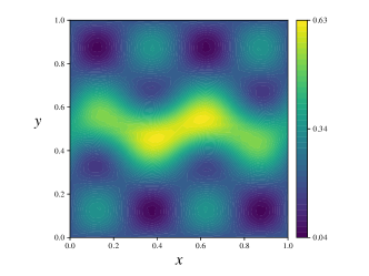
In the present experiment, we use a ground truth parameter mtruem_{\text{true}}, defined as the sum of two Gaussian-like functions to generate a data vector 𝒚\boldsymbol{y}. We depict our choice of mtruem_{\text{true}} and the corresponding state solution in Figure 1. Note that in Figure 1 (right), we also depict our choice of the subdomain Ω\Omega^{*} for the present example. Additionally, the noise variance is set to σ2=104\sigma^{2}=10^{-4}. This results in a roughly %1\%1 noise-level. As for the prior, we select the prior mean as mpr4m_{\text{pr}}\equiv 4 and use (a1,a2)=(8101,42)(a_{1},a_{2})=(8\cdot 10^{-1},4^{-2}) in (2.2). As an illustration, we visualize the MAP-point and several posterior samples in Figure 2.

Refer to caption
Figure 2: MAP point (leftmost) and three posterior samples. The posterior is obtained using data collected from the entire set of NsN_{s} candidate sensor locations.

For all numerical experiments in this paper, we use a continuous Galerkin finite element discretization with piecewise linear nodal basis functions and Nx=302N_{x}=30^{2} spatial grid points. Regarding the experimental setup, we use Ns=152N_{s}=15^{2} candidate sensor locations distributed uniformly across the domain. Implementations in the present work are conducted in python and finite element discretization is performed with FEniCS fenics2015 .

5.1.3 Optimal design and uncertainty

In what follows, we choose the spectral method for computing the classical and goal-oriented design criteria, due to its accuracy and computational efficiency. A-optimal designs are obtained by minimizing (4.12). As for the GqG_{q}-optimality criterion, we implement the spectral algorithm as outlined in Algorithm 2. Let 𝐀\mathbf{A} be the discretized version of operator 𝒜\mathcal{A} in (5.2). In the context of this problem, the GqG_{q}-optimality criterion, resulting from (4.11), is

𝚿spec,k(𝒘)=𝚪post,k𝐀𝒎pr,𝐀𝒎pr𝐌12i,j=1kγiγj𝐀𝒗i,𝒗j𝐌2.\mathbf{\Psi}_{\text{spec,k}}(\boldsymbol{w})=\left\langle\mathbf{\Gamma}_{\text{post},\text{k}}\mathbf{A}\boldsymbol{m_{\text{pr}}},\mathbf{A}\boldsymbol{m_{\text{pr}}}\right\rangle_{\mathbf{M}}-\frac{1}{2}\sum_{i,j=1}^{k}\gamma_{i}\gamma_{j}\left\langle\mathbf{A}\boldsymbol{v}_{i},\boldsymbol{v}_{j}\right\rangle_{\mathbf{M}}^{2}. (5.3)
Refer to caption
Figure 3: Classical (A-optimal) and goal-oriented (GqG_{q}-optimal) designs of size k{5,10,15,20}k\in\{5,10,15,20\} plotted over the true state solution. The subdomain Ω\Omega^{*} (black rectangles) are plotted over the goal-oriented plots.

Both classical A-optimal and goal-oriented GqG_{q}-optimal designs are obtained with the greedy algorithm. As a first illustration, we plot both types of designs over the state solution u(mtrue)u(m_{\text{true}}); see Figure 3. Note that for the GqG_{q}-optimal designs, we overlay the subdomain Ω\Omega^{*}, used in the definition of the goal-functional 𝒵\mathcal{Z} in (5.2). In Figure 3, we observe that the classical designs tend to spread over the domain, while the GqG_{q}-optimal designs cluster around the subdomain Ω\Omega^{*}. However, while the goal-oriented sensor placements prefer the subdomain, sensors are not exclusively placed within this region.

We next illustrate the effectiveness of the GqG_{q}-optimal designs in reducing the uncertainty in the goal-functional, as compared to A-optimal designs. In the left column of Figure 4, we consider posterior uncertainty in the goal-functional (top) and the inversion parameter (bottom) when using classical designs with k=5k=5 sensors. Uncertainty in the goal functional is quantified by inverting on a given design, then propagating posterior samples through the goal functional. We refer to the computed probability density function of the goal values as a goal-density. Analogous results are reported in the right column, when using goal-oriented designs. Here, the posterior distribution corresponding to each design is obtained by solving the Bayesian inverse problem, where we use data synthesized using the ground-truth parameter.

We observe that the GqG_{q}-optimal designs are far more effective in reducing posterior uncertainty in the goal-functional. The bottom row of the figure reveals that the goal-oriented designs are more effective in reducing posterior uncertainty in the inversion parameter in and around the subdomain Ω\Omega^{*}. On the other hand, the classical designs, being agnostic to the goal functional, attempt to reduce uncertainty in the inversion parameter across the domain. While this is intuitive, we point out that the nature of the goal-oriented sensor placements are not always obvious. Note that for the GqG_{q}-optimal design reported in Figure 4 (bottom-right), a sensor is placed near the right boundary. This implies that reducing uncertainty in the inversion parameter around this location is important for reducing the uncertainty in the goal-functional. In general, sensor placements are influenced by physical parameters such as the velocity field, modeling assumptions such as boundary conditions, as well as the definition of the goal-functional.

Refer to caption
Figure 4: Bottom row: classical (A-optimal) and goal-oriented (GqG_{q}-optimal) designs of size k=5k=5 plotted over the respective posterior standard deviation fields. Top row: posterior goal-densities constructed by propagating posterior samples through ZZ. The dashed line is the true goal value.

To provide further insight, we next consider classical and goal-oriented designs with varying number of sensors. Specifically, we plot the corresponding goal-densities against each other in Figure 5, as the size kk of the designs increases. We observe that the densities corresponding to the GqG_{q}-optimal designs have a smaller spread and are closer to the true goal value, when compared to the densities obtained using the A-optimal designs. This provides further evidence that our goal-oriented OED framework is more effective in reducing uncertainty in the goal-functional when compared to the classical design approach.

Refer to caption
Figure 5: Goal-densities for classical and goal-oriented approaches and k{3,4,,20}k\in\{3,4,\cdots,20\}. The dashed line is q(𝒎true)q(\boldsymbol{m_{\text{true}}}).

Next, we compare the effectiveness of classical and goal-oriented designs in terms of reducing the posterior variance in the goal-functional. Note that Theorem 3.1 provides an analytic formula for the variance of the goal with respect to a given Gaussian measure. Here, for a vector 𝒘\boldsymbol{w} of design weights, we obtain the MAP point 𝒎MAP𝒚,𝒘\boldsymbol{m_{\text{MAP}}^{\boldsymbol{y},\boldsymbol{w}}} by solving the inverse problem using data corresponding to the active sensors. Then, compute the posterior variance of the goal via

V(𝒘):=𝕍μpost{Z}=𝚪post(𝒘)𝐀𝒎MAP𝒚,𝒘,𝐀𝒎MAP𝒚,𝒘𝐌+12tr((𝚪post(𝒘)𝐀)2).V(\boldsymbol{w}):=\mathbb{V}_{\mu_{\text{post}}}\left\{Z\right\}=\left\langle\mathbf{\Gamma}_{\text{post}}(\boldsymbol{w})\mathbf{A}\boldsymbol{m_{\text{MAP}}^{\boldsymbol{y},\boldsymbol{w}}},\mathbf{A}\boldsymbol{m_{\text{MAP}}^{\boldsymbol{y},\boldsymbol{w}}}\right\rangle_{\mathbf{M}}+\frac{1}{2}\mathrm{tr}\big{(}(\mathbf{\Gamma}_{\text{post}}(\boldsymbol{w})\mathbf{A})^{2}\big{)}. (5.4)

We compute V1/2V^{1/2}, i.e., the goal standard deviation, for designs corresponding to the A-optimal and GqG_{q}-optimal designs. Additionally, we generate 100100 random weight vectors for each k{3,,20}k\in\{3,\ldots,20\} and compute the resulting values of V1/2V^{1/2}. The results of this numerical experiment are presented in Figure 6. We first observe that the goal standard deviations corresponding to the GqG_{q}-optimal designs are considerably smaller than the values for the A-optimal approach. Furthermore, both classical and goal-oriented methods out-perform the random designs in terms of uncertainty reduction. Also, note the large spread in the goal standard deviations, when using random designs.

Refer to caption
Figure 6: Standard deviations, (V(𝒘))1/2(V(\boldsymbol{w}))^{1/2}, generated with classical (A-optimal) and goal-oriented (GqG_{q}-optimal) designs of size k{3,4,,20}k\in\{3,4,\dots,20\}.

5.2 Model problem with a nonlinear goal functional

In this section, we consider an example where the goal-functional depends nonlinearly on the inversion parameter.

5.2.1 Models and goal

We consider a simplified model for the flow of a tracer through a porous medium that is saturated with a fluid. Assuming a Darcy flow model, the system is governed by the PDEs modeling fluid pressure pp and tracer concentration cc. The pressure equation is given by

(κp)\displaystyle-\nabla\cdot(\kappa\nabla p) =m,\displaystyle=m,\quad inΩ,\displaystyle\text{in}\ \Omega, (5.5)
p\displaystyle p 0,\displaystyle\equiv 0,\quad onE0p,\displaystyle\text{on}\ E_{0}^{p},
p\displaystyle p 1/2,\displaystyle\equiv 1/2,\quad onE1p,\displaystyle\text{on}\ E_{1}^{p},
p𝒏\displaystyle\nabla p\cdot\boldsymbol{n} 0,\displaystyle\equiv 0,\quad onE𝒏p.\displaystyle\text{on}\ E_{\boldsymbol{n}}^{p}.

Here, κ\kappa denotes the permeability field. The transport of the tracer is modeled by the following steady advection diffusion equation.

αΔc(cκp)\displaystyle-\alpha\Delta c-\nabla\cdot(c\kappa\nabla p) =f,in\displaystyle=f,\quad\text{in}\ Ω,\displaystyle\Omega, (5.6)
c\displaystyle c 0,on\displaystyle\equiv 0,\quad\text{on}\ E0c,\displaystyle E_{0}^{c},
c𝒏\displaystyle\nabla c\cdot\boldsymbol{n} 0,on\displaystyle\equiv 0,\quad\text{on}\ E𝒏c.\displaystyle E_{\boldsymbol{n}}^{c}.

In this equation α>0\alpha>0, is a diffusion constant and ff is a source term. Note that the velocity field in the transport equation is defined by the Darcy velocity 𝒗=κp\boldsymbol{v}=-\kappa\nabla p.

In the present example, the source term mm in (5.5) is an inversion parameter that we seek to estimate using sensor measurements of the pressure pp. Thus, the inverse problem is governed by the pressure equation (5.5), which we call the inversion model from now on. We obtain a posterior distribution for mm by solving this inverse problem. This, in turn, dictates the distribution law for the pressure field pp. Consequently, the uncertainty in mm propagates into the transport equation through the advection term in (5.5).

We define the goal-functional by

𝒵(m):=Ωc(𝒙;m)𝑑𝒙=𝟙Ω(𝒙),c(𝒙;m),\mathcal{Z}(m)\vcentcolon=\int_{\Omega^{*}}c(\boldsymbol{x};m)\,d\boldsymbol{x}=\left\langle\mathds{1}_{\Omega^{*}}(\boldsymbol{x}),c(\boldsymbol{x};m)\right\rangle, (5.7)

where ΩΩ\Omega^{*}\subset\Omega is a subdomain of interest, and 𝟙Ω\mathds{1}_{\Omega^{*}} is the indicator function of this set. Note that evaluating the goal-functional requires solving the pressure equation (5.5), followed by solving the transport equation (5.6). In what follows, we call (5.6) the prediction model.

Here, the domain Ω\Omega is chosen to be the unit square. In (5.5), we set E0pE_{0}^{p} as the right boundary and E1pE_{1}^{p} as the left boundary. Additionally, E𝒏pE_{\boldsymbol{n}}^{p} is selected as the union of the top and bottom edges of Ω\Omega. The permeability field κ(𝒙)\kappa(\boldsymbol{x}) simulates a channel or pocket of higher permeability, oriented left-to-tight across Ω\Omega. We display this field in Figure 7 (top-left).

As for the prediction model, we take E0cE_{0}^{c} to be the union of the top, bottom, and right edges of Ω\Omega, and E𝒏cE_{\boldsymbol{n}}^{c} as the left edge. The source ff in (5.6) is a single Gaussian-like function, shown in Figure 8, and the diffusion constant is set to α=0.12\alpha=0.12. Moreover, Ω\Omega^{*} is given by

Ω=D1D2,withD1=[0.18,0.32]×[0.46,0.68]andD2=[0.54,0.75]×[0.39,0.75].\Omega^{*}=D_{1}\cup D_{2},\quad\text{with}\quad D_{1}=[0.18,0.32]\times[0.46,0.68]\quad{and}\quad D_{2}=[0.54,0.75]\times[0.39,0.75].

We require a ground-truth inversion parameter mtruem_{\text{true}} for data generation. This is selected as the sum of two Gaussian-like functions, oriented asymmetrically; see Figure 7 (top-right). For the inverse problem, we set the noise variance to σ2=105\sigma^{2}=10^{-5}, resulting in approximately 1%1\% noise. The prior mean is set to the constant function mpr4m_{\text{pr}}\equiv 4. The prior covariance operator is defined according to (2.2) with (a1,a2)=(0.8,0.04)(a_{1},a_{2})=(0.8,0.04). We use Nx=302N_{x}=30^{2} finite element grid points and Ns=132N_{s}=13^{2} equally-spaced candidate sensors.

We depict the pressure field corresponding to the true parameter along with the Darcy velocity, in Figure 7 (bottom-left). The MAP point obtained by solving the inverse problem using all NsN_{s} sensors is reported in Figure 7 (bottom-right).

Refer to caption
Refer to caption
Refer to caption
Refer to caption
Figure 7: The true inversion parameter mtruem_{\text{true}} (top-left), permeability field κ(𝒙)\kappa(\boldsymbol{x}) (top-right), pressure solution p(mtrue)p(m_{\text{true}}) with Darcy velocity κ(𝒙)p-\kappa(\boldsymbol{x})\nabla p overlayed (bottom-left), and MAP-point obtained by inverting on NsN_{s} uniform sensors (bottom-right).

Recall that the goal-functional 𝒵\mathcal{Z} is formed by integrating cc over Ω\Omega^{*}, shown in Figure 9. To illustrate the dependence of 𝒵\mathcal{Z} on the inversion parameter, we plot c(p(m))c(p(m)) where mm is sampled from the posterior distribution. In particular, we generate a random design of size k=3k=3, collect data on this design, then retrieve a posterior distribution via inversion. Figure 9 shows cc corresponding to 44 posterior samples. We overlay the subdomain Ω\Omega^{*}, used to define 𝒵\mathcal{Z}.

Refer to caption
Figure 8: The source term ff in (5.6).
Refer to caption
Figure 9: Concentration field c(p(m))c(p(m)) generated with 44 posterior samples. The subdomain Ω\Omega^{*} (black rectangles) overlaid.

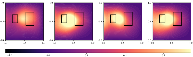
Note that due to the small amount of data used for solving the inverse problem, there is considerable variation in realizations of the concentration field.

5.2.2 Optimal designs and uncertainty

To compute GqG_{q}-optimal designs, we need to minimize the discretized goal-oriented criterion (4.2). The definition of this criterion requires the first and second order derivatives of the goal-functional, as well as an expansion point. We provide the derivation of the gradient and Hessian of 𝒵\mathcal{Z} for the present example, in a function space setting, in Appendix E. As for the expansion point, we experiment with using the prior mean as well as prior samples for m¯\bar{m}. The numerical tests that follow include testing the effectiveness of the GqG_{q}-optimal designs compared to A-optimal ones, as well as comparisons of designs obtained by minimizing the GG_{\ell}-optimality criterion. As before, we utilize the spectral method, outlined in Section 4.2, to estimate both classical and goal-oriented criteria.

Refer to caption
Figure 10: A-optimal and GqG_{q}-optimal designs of size k{5,10,15,20}k\in\{5,10,15,20\} plotted over the true pressure field p(mtrue)p(m_{\text{true}}).

Figure 10 compares A-optimal and GqG_{q}-optimal designs. Here, we use mprm_{\text{pr}} as the expansion point to form the GqG_{q}-optimality criterion. Note that, unlike the study in Section 5.1, the sensors corresponding to the goal-oriented designs do not necessarily accumulate around Ω\Omega^{*}. This indicates the non-trivial nature of such sensor placements and pitfalls of following an intuitive approach of placing sensors within Ω\Omega^{*}.

Next, we examine the effectiveness of the GqG_{q}-optimal designs in comparison to A-optimal ones. We use a prior sample as expansion point for the GqG_{q}-optimality criterion. Figure 11 presents a pairwise comparison of the goal-functional densities obtained by solving the Bayesian inverse problem with goal-oriented and classical design of various sizes.

Refer to caption
Figure 11: Goal-densities for A-optimal and GqG_{q}-optimal designs of size k{3,4,,20}k\in\{3,4,\dots,20\}. The dashed line is q(𝒎true)q(\boldsymbol{m_{\text{true}}}).

We observe that the densities corresponding to goal-oriented GqG_{q}-optimal designs have a smaller spread and tend to be closer to the true goal value in comparison to densities obtained using classical A-optimal designs. This provides further evidence that the proposed framework is more effective than the classical approach in reducing the uncertainty in the goal-functional.

5.2.3 Comparing goal-oriented OED approaches

To gain insight on the GqG_{q}-optimality and GG_{\ell}-optimality approaches, we report designs corresponding to these schemes in Figure 12. Both goal-oriented criteria are built using a prior sample for expansion point.

Refer to caption
Figure 12: Designs of size k{5,10,15,20}k\in\{5,10,15,20\} corresponding to the GqG_{q}-optimality and GG_{\ell}-optimality approaches plotted over the true pressure field p(mtrue)p(m_{\text{true}}).

We note that the GqG_{q}-optimal and GG_{\ell}-optimal designs behave similarly. This is most evident for the optimal designs of size k=5k=5. To provide a quantitative comparison of these two sensor placement strategies, we report goal-functional densities corresponding to GG_{\ell}-optimal and GqG_{q}-optimal designs in Figure 13. We use the same prior sample as the expansion point. Overall, we note that the GqG_{q}-optimal designs are more effective in reducing the uncertainty in the goal-functional compared to GG_{\ell}-optimal designs.

Refer to caption
Figure 13: Goal-densities corresponding to the GG_{\ell}-optimal and GqG_{q}-optimal designs of size k{1,2,,20}k\in\{1,2,\dots,20\}, using the prior mean as expansion point. The dashed line is the true goal value.

So far, our numerical tests correspond to comparisons with a single expansion point, being either the prior mean or a sample from the prior. To understand how results vary for different expansion points, we conduct a numerical experiment with multiple expansion points. The set of expansion points used in the following demonstration consists of the prior mean and prior samples. This study enables a thorough comparison of the proposed GqG_{q}-optimality framework against the classical A-optimal and goal-oriented GG_{\ell}-optimality approaches.

Refer to caption
Figure 14: Coefficients of variation (CV) corresponding to A-optimal, GqG_{q}-optimal, and GG_{\ell}-optimal designs of size k{3,4,,20}k\in\{3,4,\dots,20\}. Goal oriented designs are obtained using the prior mean and 2020 prior samples as expansion points.

We use the prior mean and 2020 prior samples as expansion points. These 2121 points are used to form 2121 GG_{\ell}-optimality and 21 GqG_{q}-optimality criteria. For each of the 21 expansion points, we obtain GG_{\ell}-optimal and GqG_{q}-optimal optimal designs of size k{3,4,,20}k\in\{3,4,\cdots,20\}. This results in 42 posterior distributions corresponding to each of the considered values of kk. To compare the performance of the two goal-oriented approaches, we consider a normalized notion of the posterior uncertainty in the goal-functional in each case. Specifically, we consider coefficient of variation (CV) of the goal-functional:

CV(Z):=𝕍{Z}𝔼{Z},CV(Z)\vcentcolon=\frac{\sqrt{\mathbb{V}\{Z\}}}{\mathbb{E}\{Z\}},

where 𝕍\mathbb{V} and 𝔼\mathbb{E} indicate variance and expectation with respect to the posterior distribution. We estimate the CV empirically.

For each k{3,,20}k\in\{3,\ldots,20\}, we obtain 21 CV values for the goal-functional corresponding to GG_{\ell}-optimal designs and 21 CV values for the goal-functional corresponding to GqG_{q}-optimal designs. We also compute the classical A-optimal design for each kk. The results are summarized in Figure 14. For each kk, we report the CV corresponding to the A-optimal design of size kk and pairwise box plots depicting the distribution of the CVs for the computed goal-oriented designs of size kk. It is clear from Figure 14 that, on average, both goal-oriented designs produce smaller CVs than the classical approach. Furthermore, GqG_{q}-optimal designs reduce CV the most. Additionally, we notice that choice of expansion point matters significantly for the goal-oriented schemes, especially for the GG_{\ell}-optimal designs. This is highlighted by considering the k=9k=9 case, where there is a high variance in the CVs. To illustrate this further, we isolate a subset of the design sizes and report the statistical outliers in the CV data in addition to the box plots; see Figure 15.

Refer to caption
Figure 15: A subsample of the CV’s corresponding to GG_{\ell}-optimal and GqG_{q}-optimal designs, with outliers represented as circles.

Overall, the numerical tests paint a consistent picture: (i) both types of goal-oriented designs outperform the classical designs; (ii) compared to GG_{\ell}-optimal designs, the GqG_{q}-optimal designs are more effective in reducing uncertainty in the goal functional; and (iii) compared to the GqG_{q}-optimal designs, GG_{\ell}-optimal designs show greater sensitivity to the choice of the expansion point.

6 Conclusion

In the present work, we developed a mathematical and computational framework for goal-oriented optimal of infinite-dimensional Bayesian linear inverse problems governed by PDEs. The focus is on the case where the quantity of interest defining the goal is a nonlinear functional of the inversion parameter. Our framework is based on minimizing the expected posterior variance of the quadratic approximation to the goal-functional. We refer to this as the GqG_{q}-optimality criterion. We demonstrated that this strategy outperforms classical OED, as well as c-optimal experimental design (which is based on linearization of the goal-functional), in reducing the uncertainty in the goal-functional. Additionally, the cost of our methods, measured in number of PDEs solves, are independent of the dimension of the discretized inversion parameter.

Several avenues of interest for future investigations exist on both theoretical and computational fronts. For one thing, it is natural to consider the case when the inverse problem is nonlinear. Clearly, the resulting methods would expand the application space of our goal-oriented framework. A starting point for addressing goal-oriented optimal design of nonlinear inverse problems is to consider a linearization of the parameter-to-observable mapping, resulting in locally optimal goal-oriented designs. A related approach is to use a Laplace approximation to the posterior, as is common in optimal design of infinite-dimensional inverse problems. Cases of inverse problems with potentially multi-modal designs might demand more costly strategies based on sampling. It would be interesting to investigate suitable importance sampling schemes in such contexts, for efficient evaluation of the GqG_{q}-optimality criterion.

A complementary perspective on identifying measurements that are informative to the goal-functional is a post-optimality sensitivity analysis approach. This idea was used in SunseriHartVanBloemenWaandersAlexanderian20 to identify measurements that are most influential to the solution of a deterministic inverse problem. Such ideas were extended to cases of Bayesian inverse problems governed by PDEs in SunseriAlexanderianHartEtAl24 ; ChowdharyTongStadlerEtAl24 . This approach can also be used in a goal-oriented manner. Namely, one can consider the sensitivity of measures of uncertainty in the goal-functional to different measurements to identify informative experiments. This is particularly attractive in the case of nonlinear inverse problems governed by PDEs.

Another important line of inquiry is to investigate goal-oriented criteria defined in terms of quantities other than the posterior variance. For example, one can seek designs that maximize information gain regarding the goal-functional or optimizing inference of the tail behavior of the goal-functional. A yet another potential avenue of further investigations is considering relaxation strategies to replace the binary goal-oriented optimization problem with a continuous optimization problem, for which powerful gradient-based optimization methods maybe deployed.

Acknowledgments

This article has been authored by employees of National Technology & Engineering Solutions of Sandia, LLC under Contract No. DE-NA0003525 with the U.S. Department of Energy (DOE). The employees own all right, title and interest in and to the article and are solely responsible for its contents. SAND2024-15167O.

This material is also based upon work supported by the U.S. Department of Energy, Office of Science, Office of Advanced Scientific Computing Research Field Work Proposal Number 23-02526.

References

  • [1] A. Alexanderian. Optimal experimental design for infinite-dimensional Bayesian inverse problems governed by PDEs: A review. Inverse Problems, 37(4), 2021.
  • [2] A. Alexanderian, P. J. Gloor, and O. Ghattas. On Bayesian A- and D-Optimal Experimental Designs in Infinite Dimensions. Bayesian Analysis, 11(3), 2016.
  • [3] A. Alexanderian, N. Petra, G. Stadler, and O. Ghattas. A-optimal design of experiments for infinite-dimensional Bayesian linear inverse problems with regularized 0\ell_{0}-sparsification. SIAM Journal Scientific Computing, 36(5):A2122–A2148, 2014.
  • [4] A. Alexanderian, N. Petra, G. Stadler, and O. Ghattas. A fast and scalable method for A-optimal design of experiments for infinite-dimensional Bayesian nonlinear inverse problems. SIAM Journal Scientific Computing, 38(1):A243–A272, 2016.
  • [5] A. Alexanderian, N. Petra, G. Stadler, and O. Ghattas. Mean-variance risk-averse optimal control of systems governed by PDEs with random parameter fields using quadratic approximations. SIAM/ASA Journal on Uncertainty Quantification, 5(1):1166–1192, 2017.
  • [6] A. Alexanderian and A. K. Saibaba. Efficient D-optimal design of experiments for infinite-dimensional Bayesian linear inverse problems. SIAM Journal Scientific Computing, 40(5):A2956–A2985, 2018.
  • [7] M. Alnæs, J. Blechta, J. Hake, A. Johansson, B. Kehlet, A. Logg, C. Richardson, J. Ring, M. E. Rognes, and G. N. Wells. The fenics project version 1.5. Archive of numerical software, 3(100), 2015.
  • [8] A. C. Atkinson and A. N. Donev. Optimum Experimental Designs. Oxford, 1992.
  • [9] A. Attia, A. Alexanderian, and A. K. Saibaba. Goal-oriented optimal design of experiments for large-scale Bayesian linear inverse problems. Inverse Problems, 34(9):095009, 2018.
  • [10] H. Avron and S. Toledo. Randomized algorithms for estimating the trace of an implicit symmetric positive semi-definite matrix. Journal of the ACM, 58(2):34, 2011.
  • [11] T. Bui-Thanh, O. Ghattas, J. Martin, and G. Stadler. A computational framework for infinite-dimensional Bayesian inverse problems. Part I: The linearized case, with application to global seismic inversion. SIAM Journal on Scientific Computing, 35(6):A2494–A2523, 2013.
  • [12] T. Butler, J. Jakeman, and T. Wildey. Combining push-forward measures and Bayes’ rule to construct consistent solutions to stochastic inverse problems. SIAM Journal on Scientific Computing, 40(2):A984–A1011, 2018.
  • [13] T. Butler, J. D. Jakeman, and T. Wildey. Optimal experimental design for prediction based on push-forward probability measures. Journal of Computational Physics, 416:109518, 2020.
  • [14] K. Chaloner and I. Verdinelli. Bayesian experimental design: A review. Statistical Science, 10(3):273–304, 1995.
  • [15] A. Chowdhary, S. Tong, G. Stadler, and A. Alexanderian. Sensitivity analysis of the information gain in infinite-dimensional Bayesian linear inverse problems. International Journal for Uncertainty Quantification, 14(6), 2024.
  • [16] G. Da Prato. An introduction to infinite-dimensional analysis. Springer, 2006.
  • [17] G. Da Prato and J. Zabczyk. Second-order partial differential equations in Hilbert spaces. Cambridge University Press, 2002.
  • [18] M. Dashti and A. M. Stuart. The Bayesian approach to inverse problems. In R. Ghanem, D. Higdon, and H. Owhadi, editors, Handbook of Uncertainty Quantification, pages 311–428. Spinger, 2017.
  • [19] E. Haber, L. Horesh, and L. Tenorio. Numerical methods for experimental design of large-scale linear ill-posed inverse problems. Inverse Problems, 24(055012):125–137, 2008.
  • [20] E. Haber, Z. Magnant, C. Lucero, and L. Tenorio. Numerical methods for A-optimal designs with a sparsity constraint for ill-posed inverse problems. Computational Optimization and Applications, pages 1–22, 2012.
  • [21] N. Halko, P.-G. Martinsson, and J. A. Tropp. Finding structure with randomness: Probabilistic algorithms for constructing approximate matrix decompositions. SIAM Review, 53(2):217–288, 2011.
  • [22] E. Herman, A. Alexanderian, and A. K. Saibaba. Randomization and reweighted 1\ell_{1}-minimization for A-optimal design of linear inverse problems. SIAM Journal on Scientific Computing, 42(3):A1714–A1740, 2020.
  • [23] R. Herzog, I. Riedel, and D. Uciński. Optimal sensor placement for joint parameter and state estimation problems in large-scale dynamical systems with applications to thermo-mechanics. Optimization and Engineering, 19:591–627, 2018.
  • [24] B. Holmquist. Moments and cumulants of the multivariate normal distribution. Stochastic Analysis and Applications, 6(3):273–278, 1988.
  • [25] F. Li. A combinatorial approach to goal-oriented optimal Bayesian experimental design. PhD thesis, Massachusetts Institute of Technology, 2019.
  • [26] F. Pukelsheim. Optimal design of experiments. SIAM, 2006.
  • [27] A. M. Stuart. Inverse problems: A Bayesian perspective. Acta Numerica, 19:451–559, 2010.
  • [28] I. Sunseri, A. Alexanderian, J. Hart, and B. van Bloemen Waanders. Hyper-differential sensitivity analysis for nonlinear Bayesian inverse problems. International Journal for Uncertainty Quantification, 14(2), 2024.
  • [29] I. Sunseri, J. Hart, B. van Bloemen Waanders, and A. Alexanderian. Hyper-differential sensitivity analysis for inverse problems constrained by partial differential equations. Inverse Problems, 2020.
  • [30] K. Triantafyllopoulos. Moments and cumulants of the multivariate real and complex gaussian distributions, 2002.
  • [31] F. Tröltzsch. Optimal Control of Partial Differential Equations: Theory, Methods and Applications, volume 112 of Graduate Studies in Mathematics. American Mathematical Society, 2010.
  • [32] D. Uciński. Optimal measurement methods for distributed parameter system identification. CRC Press, Boca Raton, 2005.
  • [33] U. Villa, N. Petra, and O. Ghattas. hIPPYlib: An extensible software framework for large-scale inverse problems governed by PDEs: Part I: Deterministic inversion and linearized Bayesian inference. ACM Transactions on Mathematical Software (TOMS), 47(2):1–34, 2021.
  • [34] C. S. Withers. The moments of the multivariate normal. Bulletin of the Australian Mathematical Society, 32(1):103–107, 1985.
  • [35] K. Wu, P. Chen, and O. Ghattas. An offline-online decomposition method for efficient linear Bayesian goal-oriented optimal experimental design: Application to optimal sensor placement. SIAM Journal on Scientific Computing, 45(1):B57–B77, 2023.

Appendix A Proof of Theorem 3.1

We first recall some notations and definitions regarding Gaussian measures on Hilbert spaces. Recall that for a Gaussian measure μ=𝖭(m0,𝒞)\mu=\mathsf{N}(m_{0},\mathcal{C}) on a real separable Hilbert space \mathscr{M} the mean m0m_{0}\in\mathscr{M} satisfies,

m0,v=s,vμ(ds),for all v.\left\langle m_{0},v\right\rangle=\int_{\mathscr{M}}\left\langle s,v\right\rangle\mu(ds),\quad\text{for all }v\in\mathscr{M}.

Moreover, 𝒞\mathcal{C} is a positive self-adjoint trace class operator that satisfies,

𝒞u,v=u,sm0v,sm0μ(ds).\left\langle\mathcal{C}u,v\right\rangle=\int_{\mathscr{M}}\left\langle u,s-m_{0}\right\rangle\left\langle v,s-m_{0}\right\rangle\,\mu(ds). (A.1)

For further details, see [16, Section 1.4]. We assume that 𝒞\mathcal{C} is strictly positive. In what follows, we let {ei}i\{e_{i}\}_{i\in\mathbb{N}} be the complete orthonormal set of eigenvectors of 𝒞\mathcal{C} and {λi}i\{\lambda_{i}\}_{i\in\mathbb{N}} the corresponding (real and positive) eigenvalues.

Consider the probability space (,(),μ)(\mathscr{M},\mathscr{B}(\mathscr{M}),\mu), where \mathscr{B} is the Borel σ\upsigma-algebra on \mathscr{M}. For a fixed vv\in\mathscr{M}, the linear functional

φ(s)=s,v,s,\varphi(s)=\left\langle s,v\right\rangle,\quad s\in\mathscr{M},

considered as a random variable φ:(,(),μ)(,())\varphi:(\mathscr{M},\mathscr{B}(\mathscr{M}),\mu)\to(\mathbb{R},\mathscr{B}(\mathbb{R})), is a Gaussian random variable with mean φ(m0)\varphi(m_{0}) and variance σv2=𝒞v,v\sigma^{2}_{v}=\left\langle\mathcal{C}v,v\right\rangle. More generally, for v1,,vnv_{1},\ldots,v_{n} in \mathscr{M}, the random nn-vector 𝒀:n\boldsymbol{Y}:\mathscr{M}\to\mathbb{R}^{n} given by 𝒀(s)=[s,v1s,v2s,vn]\boldsymbol{Y}(s)=[\left\langle s,v_{1}\right\rangle\;\left\langle s,v_{2}\right\rangle\;\ldots\;\left\langle s,v_{n}\right\rangle]^{\top} is an nn-variate Gaussian whose distribution law is 𝖭(𝒚¯,𝐂)\mathsf{N}(\bar{\boldsymbol{y}},\mathbf{C}),

y¯i=m0,vi,Cij=𝒞vi,vj,i,j{1,,n}.\bar{y}_{i}=\left\langle m_{0},v_{i}\right\rangle,\quad C_{ij}=\left\langle\mathcal{C}v_{i},v_{j}\right\rangle,\quad i,j\in\{1,\ldots,n\}. (A.2)

The arguments in this appendix rely heavily on the standard approach of using finite-dimensional projections to facilitate computation of Gaussian integrals. As such we also need some basic background results regarding Gaussian random vectors. In particular, we need the following result [34, 24, 30].

Lemma 1

Suppose 𝐘𝖭(𝟎,𝐂)\boldsymbol{Y}\sim\mathsf{N}(\boldsymbol{0},\mathbf{C}) is an nn-variate Gaussian random variable. Then, for i,j,ki,j,k, and \ell in {1,,n}\{1,\ldots,n\},

  1. (a)

    𝔼{YiYjYk}=0\mathbb{E}\{Y_{i}Y_{j}Y_{k}\}=0; and

  2. (b)

    𝔼{YiYjYkY}=CijCk+CikCj+CiCjk\mathbb{E}\{Y_{i}Y_{j}Y_{k}Y_{\ell}\}=C_{ij}C_{k\ell}+C_{ik}C_{j\ell}+C_{i\ell}C_{jk}.

The following technical result is useful in what follows.

Lemma 2

Let 𝒜\mathcal{A} be a bounded selfadjoint linear operator on a Hilbert space \mathscr{M}, and let μ0:=𝖭(0,𝒞)\mu_{0}:=\mathsf{N}(0,\mathcal{C}) be a Gaussian measure on \mathscr{M}. We have

  1. (a)

    b,sc,sμ0(ds)=𝒞b,c\int_{\mathscr{M}}\left\langle b,s\right\rangle\left\langle c,s\right\rangle\,\mu_{0}(ds)=\left\langle\mathcal{C}b,c\right\rangle, for all bb and cc in \mathscr{M};

  2. (b)

    𝒜s,sb,sμ0(ds)=0\int_{\mathscr{M}}\left\langle\mathcal{A}s,s\right\rangle\left\langle b,s\right\rangle\,\mu_{0}(ds)=0, for all bb\in\mathscr{M}; and

  3. (c)

    𝒜s,s2μ0(ds)=(tr(𝒞𝒜))2+2tr((𝒞𝒜)2)\int_{\mathscr{M}}\left\langle\mathcal{A}s,s\right\rangle^{2}\,\mu_{0}(ds)=\big{(}\mathrm{tr}(\mathcal{C}\mathcal{A})\big{)}^{2}+2\mathrm{tr}\big{(}(\mathcal{C}\mathcal{A})^{2}\big{)}.

Proof

The first statement follows immediately from (A.1). We consider (b) next. For nn\in\mathbb{N}, we define the projector πn\pi_{n} in terms of the eigenvectors of 𝒞\mathcal{C},

πn(s):=i=1ns,eiei,s.\pi_{n}(s):=\sum_{i=1}^{n}\left\langle s,e_{i}\right\rangle e_{i},\quad s\in\mathscr{M}.

Note that 𝒀:(,(),μ0)(n,(n))\boldsymbol{Y}:(\mathscr{M},\mathscr{B}(\mathscr{M}),\mu_{0})\to(\mathbb{R}^{n},\mathscr{B}(\mathbb{R}^{n})) defined by 𝒀(s):=[s,e1s,e2s,en]\boldsymbol{Y}(s)\vcentcolon=[\left\langle s,e_{1}\right\rangle\;\left\langle s,e_{2}\right\rangle\;\ldots\;\left\langle s,e_{n}\right\rangle]^{\top} has an nn-variate Gaussian law, 𝒀𝖭(𝟎,𝐂)\boldsymbol{Y}\sim\mathsf{N}(\boldsymbol{0},\mathbf{C}), with

Cij=𝒞ei,ej=λiδij,C_{ij}=\left\langle\mathcal{C}e_{i},e_{j}\right\rangle=\lambda_{i}\delta_{ij},

where δij\delta_{ij} is the Kronecker delta. We next consider,

𝒜s,sb,s=limnτn(s)whereτn(s):=𝒜πn(s),πn(s)b,πn(s).\left\langle\mathcal{A}s,s\right\rangle\left\langle b,s\right\rangle=\lim_{n\rightarrow\infty}\tau_{n}(s)\quad\text{where}\quad\tau_{n}(s)\vcentcolon=\left\langle\mathcal{A}\pi_{n}(s),\pi_{n}(s)\right\rangle\left\langle b,\pi_{n}(s)\right\rangle.

Note that for each nn\in\mathbb{N},

τn(s)μ0(ds)=i,j,k=1n𝒜ei,ejb,eks,eis,ejs,ekμ0(ds)=i,j,k=1n𝒜ei,ej𝔼{YiYjYk}=0.\int_{\mathscr{M}}\tau_{n}(s)\,\mu_{0}(ds)=\sum_{i,j,k=1}^{n}\left\langle\mathcal{A}e_{i},e_{j}\right\rangle\left\langle b,e_{k}\right\rangle\int_{\mathscr{M}}\left\langle s,e_{i}\right\rangle\left\langle s,e_{j}\right\rangle\left\langle s,e_{k}\right\rangle\,\mu_{0}(ds)=\sum_{i,j,k=1}^{n}\left\langle\mathcal{A}e_{i},e_{j}\right\rangle\mathbb{E}\{Y_{i}Y_{j}Y_{k}\}=0.

The last step follows from Lemma 1(a). Furthermore, |τn(s)|𝒜bπn(s)3𝒜bs3|\tau_{n}(s)|\leq\|\mathcal{A}\|\|b\|\|\pi_{n}(s)\|^{3}\leq\|\mathcal{A}\|\|b\|\|s\|^{3}, for all nn\in\mathbb{N}. Therefore, since s3μ0(ds)<\int_{\mathscr{M}}\|s\|^{3}\,\mu_{0}(ds)<\infty, by the Dominated Convergence Theorem,

𝒜s,sb,sμ0(ds)=limnτn(s)μ0(ds)=limnτn(s)μ0(ds)=0.\int_{\mathscr{M}}\left\langle\mathcal{A}s,s\right\rangle\left\langle b,s\right\rangle\,\mu_{0}(ds)=\int_{\mathscr{M}}\lim_{n\rightarrow\infty}\tau_{n}(s)\,\mu_{0}(ds)=\lim_{n\rightarrow\infty}\int_{\mathscr{M}}\tau_{n}(s)\,\mu_{0}(ds)=0.

We next consider the third statement of the lemma. The approach is similar to the proof of part (b). We note that

𝒜s,s2=limnθn(s)whereθn(s):=𝒜πn(s),πn(s)2.\left\langle\mathcal{A}s,s\right\rangle^{2}=\lim_{n\rightarrow\infty}\theta_{n}(s)\quad\text{where}\quad\theta_{n}(s):=\left\langle\mathcal{A}\pi_{n}(s),\pi_{n}(s)\right\rangle^{2}.

As in the case of τn\tau_{n} above, we can easily bound θn\theta_{n}. Specifically, |θn(s)|𝒜2s4|\theta_{n}(s)|\leq\|\mathcal{A}\|^{2}\|s\|^{4}, for all nn\in\mathbb{N}. Note also that s4μ0(ds)<\int_{\mathscr{M}}\|s\|^{4}\,\mu_{0}(ds)<\infty. Therefore, by the Dominated Convergence Theorem,

𝒜s,s2μ0(ds)=limnθn(s)μ0(ds)=limnθn(s)μ0(ds).\int_{\mathscr{M}}\left\langle\mathcal{A}s,s\right\rangle^{2}\,\mu_{0}(ds)=\int_{\mathscr{M}}\lim_{n\rightarrow\infty}\theta_{n}(s)\,\mu_{0}(ds)=\lim_{n\rightarrow\infty}\int_{\mathscr{M}}\theta_{n}(s)\,\mu_{0}(ds). (A.3)

Next, note that for each nn,

θn(s)μ0(ds)\displaystyle\int_{\mathscr{M}}\theta_{n}(s)\,\mu_{0}(ds) =i,j,k,=1n𝒜ei,ej𝒜ek,es,eis,ejs,eks,eμ0(ds)\displaystyle=\sum_{{i},{j},{k},{\ell}=1}^{n}\left\langle\mathcal{A}e_{{i}},e_{{j}}\right\rangle\left\langle\mathcal{A}e_{{k}},e_{{\ell}}\right\rangle\int_{\mathscr{M}}\left\langle s,e_{i}\right\rangle\left\langle s,e_{j}\right\rangle\left\langle s,e_{k}\right\rangle\left\langle s,e_{\ell}\right\rangle\,\mu_{0}(ds)
=i,j,k,=1n𝒜ei,ej𝒜ek,e(CijCk+CikCj+CiCjk),\displaystyle=\sum_{{i},{j},{k},{\ell}=1}^{n}\left\langle\mathcal{A}e_{{i}},e_{{j}}\right\rangle\left\langle\mathcal{A}e_{{k}},e_{{\ell}}\right\rangle(C_{ij}C_{k\ell}+C_{ik}C_{j\ell}+C_{i\ell}C_{jk}), (A.4)

where we have used Lemma 1(b) in the final step. Let us consider each of the three terms in (A.4). We note,

i,j,k,=1n𝒜ei,ej𝒜ek,eCijCk\displaystyle\sum_{i,j,k,\ell=1}^{n}\left\langle\mathcal{A}e_{i},e_{j}\right\rangle\left\langle\mathcal{A}e_{k},e_{\ell}\right\rangle C_{ij}C_{k\ell} =i,j,k,nλjλk𝒜ei,ej𝒜ek,eδijδk\displaystyle=\sum_{i,j,k,\ell}^{n}\lambda_{j}\lambda_{k}\left\langle\mathcal{A}e_{i},e_{j}\right\rangle\left\langle\mathcal{A}e_{k},e_{\ell}\right\rangle\delta_{ij}\delta_{k\ell}
=i,k=1nλiλk𝒜ei,ei𝒜ek,ek\displaystyle=\sum_{i,k=1}^{n}\lambda_{i}\lambda_{k}\left\langle\mathcal{A}e_{i},e_{i}\right\rangle\left\langle\mathcal{A}e_{k},e_{k}\right\rangle
=(i=1nλi𝒜ei,ei)2\displaystyle=\left(\sum_{i=1}^{n}\lambda_{i}\left\langle\mathcal{A}e_{i},e_{i}\right\rangle\right)^{2}
=(i=1n𝒜ei,,𝒞ei)2(tr(𝒞𝒜))2,as n.\displaystyle=\left(\sum_{i=1}^{n}\left\langle\mathcal{A}e_{i,},\mathcal{C}e_{i}\right\rangle\right)^{2}\to\big{(}\mathrm{tr}(\mathcal{C}\mathcal{A})\big{)}^{2},\quad\text{as }n\to\infty. (A.5)

Before, we consider the second and third terms in (A.4), we note

tr((𝒜𝒞)2)=tr(𝒜𝒞𝒜𝒞)=i=1ei,𝒜𝒞𝒜𝒞ei=i=1λiei,𝒜𝒞𝒜ei=i=1λiei,𝒜𝒞(j=1𝒜ei,ejej)=i,j=1λiei,𝒜𝒞ej𝒜ei,ej=i,j=1λiλj𝒜ei,ej2.\mathrm{tr}\big{(}(\mathcal{A}\mathcal{C})^{2}\big{)}=\mathrm{tr}(\mathcal{A}\mathcal{C}\mathcal{A}\mathcal{C})=\sum_{i=1}^{\infty}\left\langle e_{i},\mathcal{A}\mathcal{C}\mathcal{A}\mathcal{C}e_{i}\right\rangle=\sum_{i=1}^{\infty}\lambda_{i}\left\langle e_{i},\mathcal{A}\mathcal{C}\mathcal{A}e_{i}\right\rangle=\sum_{i=1}^{\infty}\lambda_{i}\left\langle e_{i},\mathcal{A}\mathcal{C}\big{(}\sum_{j=1}^{\infty}\left\langle\mathcal{A}e_{i},e_{j}\right\rangle e_{j}\big{)}\right\rangle\\ =\sum_{i,j=1}^{\infty}\lambda_{i}\left\langle e_{i},\mathcal{A}\mathcal{C}e_{j}\right\rangle\left\langle\mathcal{A}e_{i},e_{j}\right\rangle=\sum_{i,j=1}^{\infty}\lambda_{i}\lambda_{j}\left\langle\mathcal{A}e_{i},e_{j}\right\rangle^{2}.

Next, we note

i,j,k,=1n𝒜ei,ej𝒜ek,eCikCj=i,j,k,=1nλiλj𝒜ei,ej𝒜ek,eδikδj=i,j=1nλiλj𝒜ei,ej2tr((𝒜𝒞)2),\sum_{i,j,k,\ell=1}^{n}\left\langle\mathcal{A}e_{i},e_{j}\right\rangle\left\langle\mathcal{A}e_{k},e_{\ell}\right\rangle C_{ik}C_{j\ell}=\sum_{i,j,k,\ell=1}^{n}\lambda_{i}\lambda_{j}\left\langle\mathcal{A}e_{i},e_{j}\right\rangle\left\langle\mathcal{A}e_{k},e_{\ell}\right\rangle\delta_{ik}\delta_{j\ell}=\sum_{i,j=1}^{n}\lambda_{i}\lambda_{j}\left\langle\mathcal{A}e_{i},e_{j}\right\rangle^{2}\to\mathrm{tr}\big{(}(\mathcal{A}\mathcal{C})^{2}\big{)}, (A.6)

as nn\to\infty. A similar argument shows,

i,j,k,=1n𝒜ei,ej𝒜ek,eCiCjk=i,j=1nλiλj𝒜ei,ej2tr((𝒜𝒞)2),as n.\sum_{i,j,k,\ell=1}^{n}\left\langle\mathcal{A}e_{i},e_{j}\right\rangle\left\langle\mathcal{A}e_{k},e_{\ell}\right\rangle C_{i\ell}C_{jk}=\sum_{i,j=1}^{n}\lambda_{i}\lambda_{j}\left\langle\mathcal{A}e_{i},e_{j}\right\rangle^{2}\to\mathrm{tr}\big{(}(\mathcal{A}\mathcal{C})^{2}\big{)},\quad\text{as }n\to\infty. (A.7)

Hence, combining (A.3)–(A.7), we obtain

𝒜s,s2μ0(ds)=limnθn(s)μ0(ds)=limnθn(s)μ0(ds)=(tr(𝒞𝒜))2+2tr((𝒞𝒜)2),\int_{\mathscr{M}}\left\langle\mathcal{A}s,s\right\rangle^{2}\,\mu_{0}(ds)=\int_{\mathscr{M}}\lim_{n\rightarrow\infty}\theta_{n}(s)\,\mu_{0}(ds)=\lim_{n\rightarrow\infty}\int_{\mathscr{M}}\theta_{n}(s)\,\mu_{0}(ds)=\big{(}\mathrm{tr}(\mathcal{C}\mathcal{A})\big{)}^{2}+2\mathrm{tr}\big{(}(\mathcal{C}\mathcal{A})^{2}\big{)},

which completes the proof of the lemma. \square

The following result extends Lemma 2 to the case of non-centered Gaussian measures.

Lemma 3

Let 𝒜\mathcal{A} be a bounded selfadjoint linear operator on a real Hilbert space \mathscr{M}, and let μ:=𝖭(m0,𝒞)\mu:=\mathsf{N}(m_{0},\mathcal{C}) be a Gaussian measure on \mathscr{M}.

  1. (a)

    b,sc,sμ(ds)=𝒞b,c+b,m0c,m0\int_{\mathscr{M}}\left\langle b,s\right\rangle\left\langle c,s\right\rangle\,\mu(ds)=\left\langle\mathcal{C}b,c\right\rangle+\left\langle b,m_{0}\right\rangle\left\langle c,m_{0}\right\rangle, for all bb and cc in \mathscr{M};

  2. (b)

    𝒜s,sb,sμ(ds)=(𝒜m0,m0+tr(𝒞𝒜))b,m0+2𝒞𝒜m0,b\int_{\mathscr{M}}\left\langle\mathcal{A}s,s\right\rangle\left\langle b,s\right\rangle\,\mu(ds)=\big{(}\!\left\langle\mathcal{A}m_{0},m_{0}\right\rangle+\mathrm{tr}(\mathcal{C}\mathcal{A})\big{)}\left\langle b,m_{0}\right\rangle+2\left\langle\mathcal{C}\mathcal{A}m_{0},b\right\rangle for all bb\in\mathscr{M}; and

  3. (c)

    𝒜s,s2μ(ds)=(tr(𝒞𝒜))2+2tr((𝒞𝒜)2)+4𝒞𝒜m0,𝒜m0+(𝒜m0,m0+2tr(𝒞𝒜))𝒜m0,m0\int_{\mathscr{M}}\left\langle\mathcal{A}s,s\right\rangle^{2}\,\mu(ds)=\big{(}\mathrm{tr}(\mathcal{C}\mathcal{A})\big{)}^{2}+2\mathrm{tr}\big{(}(\mathcal{C}\mathcal{A})^{2}\big{)}+4\left\langle\mathcal{C}\mathcal{A}m_{0},\mathcal{A}m_{0}\right\rangle+\left(\left\langle\mathcal{A}m_{0},m_{0}\right\rangle+2\mathrm{tr}\left(\mathcal{C}\mathcal{A}\right)\right)\left\langle\mathcal{A}m_{0},m_{0}\right\rangle.

Proof

These identities follow from Lemma 2 and some basic manipulations. For brevity, we only prove the third statement. The other two can be derived similarly. Using Lemma 2(c),

𝒜(sm0),sm02μ(ds)\displaystyle\int_{\mathscr{M}}\left\langle\mathcal{A}(s-m_{0}),s-m_{0}\right\rangle^{2}\,\mu(ds) =(tr(𝒞𝒜))2+2tr((𝒞𝒜)2)\displaystyle=\big{(}\mathrm{tr}(\mathcal{C}\mathcal{A})\big{)}^{2}+2\mathrm{tr}\big{(}(\mathcal{C}\mathcal{A})^{2}\big{)}
=𝒜s,s2μ(ds)+4𝒜m0,s2μ(ds)+𝒜m0,m02\displaystyle=\int_{\mathscr{M}}\left\langle\mathcal{A}s,s\right\rangle^{2}\,\mu(ds)+4\int_{\mathscr{M}}\left\langle\mathcal{A}m_{0},s\right\rangle^{2}\,\mu(ds)+\left\langle\mathcal{A}m_{0},m_{0}\right\rangle^{2}
4𝒜s,s𝒜m0,sμ(ds)4𝒜m0,s𝒜m0,m0μ(ds)\displaystyle\quad-4\int_{\mathscr{M}}\left\langle\mathcal{A}s,s\right\rangle\left\langle\mathcal{A}m_{0},s\right\rangle\,\mu(ds)-4\int_{\mathscr{M}}\left\langle\mathcal{A}m_{0},s\right\rangle\left\langle\mathcal{A}m_{0},m_{0}\right\rangle\,\mu(ds)
+2𝒜s,s𝒜m0,m0μ(ds).\displaystyle\quad+2\int_{\mathscr{M}}\left\langle\mathcal{A}s,s\right\rangle\left\langle\mathcal{A}m_{0},m_{0}\right\rangle\,\mu(ds).

Subsequently, we solve for 𝒜s,s2μ(ds)\int_{\mathscr{M}}\left\langle\mathcal{A}s,s\right\rangle^{2}\,\mu(ds). To do this, we require the formula for the expected value of a quadratic form on a Hilbert space (see [2, Lemma 1]) and items (a) and (b) of the present lemma. Performing the calculation, we arrive at

𝒜m,m2μ(ds)=(tr(𝒞𝒜))2+2tr((𝒞𝒜)2)+4𝒞𝒜m0,𝒜m0+(𝒜m0,m0+2tr(𝒞𝒜))𝒜m0,m0.\int_{\mathscr{M}}\left\langle\mathcal{A}m,m\right\rangle^{2}\,\mu(ds)=\big{(}\mathrm{tr}(\mathcal{C}\mathcal{A})\big{)}^{2}+2\mathrm{tr}\big{(}(\mathcal{C}\mathcal{A})^{2}\big{)}+4\left\langle\mathcal{C}\mathcal{A}m_{0},\mathcal{A}m_{0}\right\rangle+\left(\left\langle\mathcal{A}m_{0},m_{0}\right\rangle+2\mathrm{tr}\left(\mathcal{C}\mathcal{A}\right)\right)\left\langle\mathcal{A}m_{0},m_{0}\right\rangle.

\square

We now have all the tools required to prove Theorem 3.1.

Proof (Proof of Theorem 3.1)

Consider (3.7). Note that

𝕍μ{𝒵}=𝔼μ{𝒵2}(𝔼μ{𝒵})2.\mathbb{V}_{\mu}\left\{\mathcal{Z}\right\}=\mathbb{E}_{\mu}\left\{\mathcal{Z}^{2}\right\}-\big{(}\mathbb{E}_{\mu}\{\mathcal{Z}\}\big{)}^{2}. (A.8)

The second term of (A.8) is straightforward to compute. Specifically,

𝔼μ{𝒵}=𝒵(m)μ(dm)=12𝒜m,mμ(dm)+b,mμ(dm)=12(𝒜m0,m0+tr(𝒞𝒜))+b,m0.\mathbb{E}_{\mu}\{\mathcal{Z}\}=\int_{\mathscr{M}}\mathcal{Z}(m)\,\mu(dm)=\frac{1}{2}\int_{\mathscr{M}}\left\langle\mathcal{A}m,m\right\rangle\mu(dm)+\int_{\mathscr{M}}\left\langle b,m\right\rangle\,\mu(dm)=\frac{1}{2}\left(\left\langle\mathcal{A}m_{0},m_{0}\right\rangle+\mathrm{tr}\left(\mathcal{C}\mathcal{A}\right)\right)+\left\langle b,m_{0}\right\rangle. (A.9)

Computing the first term in (A.8) is facilitated by Lemma 3. We note

𝔼μ{𝒵2}\displaystyle\mathbb{E}_{\mu}\{\mathcal{Z}^{2}\} =𝒵(m)2μ(dm)\displaystyle=\int_{\mathscr{M}}\mathcal{Z}(m)^{2}\,\mu(dm)
=14𝒜m,m2μ(dm)+𝒜m,mb,mμ(dm)+b,m2μ(dm)\displaystyle=\frac{1}{4}\int_{\mathscr{M}}\left\langle\mathcal{A}m,m\right\rangle^{2}\,\mu(dm)+\int_{\mathscr{M}}\left\langle\mathcal{A}m,m\right\rangle\left\langle b,m\right\rangle\,\mu(dm)+\int_{\mathscr{M}}\left\langle b,m\right\rangle^{2}\,\mu(dm)
=14𝒜m0,m02+𝒜m0,m0b,m0+𝒞𝒜m0,𝒜m0\displaystyle=\frac{1}{4}\left\langle\mathcal{A}m_{0},m_{0}\right\rangle^{2}+\left\langle\mathcal{A}m_{0},m_{0}\right\rangle\left\langle b,m_{0}\right\rangle+\left\langle\mathcal{C}\mathcal{A}m_{0},\mathcal{A}m_{0}\right\rangle
+2𝒞𝒜m0,b+b,m02+𝒞b,b\displaystyle\quad+2\left\langle\mathcal{C}\mathcal{A}m_{0},b\right\rangle+\left\langle b,m_{0}\right\rangle^{2}+\left\langle\mathcal{C}b,b\right\rangle
+(𝒜m0,m0+b,m0)tr(𝒞𝒜)\displaystyle\quad+\left(\left\langle\mathcal{A}m_{0},m_{0}\right\rangle+\left\langle b,m_{0}\right\rangle\right)\mathrm{tr}\left(\mathcal{C}\mathcal{A}\right)
+14(tr(𝒞𝒜))2+12tr((𝒞𝒜)2).\displaystyle\quad+\frac{1}{4}\big{(}\mathrm{tr}(\mathcal{C}\mathcal{A})\big{)}^{2}+\frac{1}{2}\mathrm{tr}\big{(}(\mathcal{C}\mathcal{A})^{2}\big{)}.

Substituting this and (A.9) into (A.8) and simplifying provides the desired identity for 𝕍μ{𝒵}\mathbb{V}_{\mu}\{\mathcal{Z}\}. \square

Appendix B Proof of Theorem 3.2

Proof (Proof of Theorem 3.2)

We begin with the following definitions

𝒜:=¯𝒵,b:=g¯𝒵¯𝒵m¯,c:=𝒵(m¯)g¯𝒵,m¯+12¯𝒵m¯,m¯.\mathcal{A}\vcentcolon=\bar{\mathcal{H}}_{\scriptscriptstyle{\mathcal{Z}}},\quad b\vcentcolon=\bar{g}_{\scriptscriptstyle{\mathcal{Z}}}-\bar{\mathcal{H}}_{\scriptscriptstyle{\mathcal{Z}}}\bar{m},\quad c\vcentcolon=\mathcal{Z}(\bar{m})-\left\langle\bar{g}_{\scriptscriptstyle{\mathcal{Z}}},\bar{m}\right\rangle+\frac{1}{2}\left\langle\bar{\mathcal{H}}_{\scriptscriptstyle{\mathcal{Z}}}\bar{m},\bar{m}\right\rangle. (B.1)

These components enable expressing 𝒵quad\mathcal{Z}_{\text{quad}} as

𝒵quad(m)=12𝒜m,m+b,m+c.\mathcal{Z}_{\text{quad}}(m)=\frac{1}{2}\left\langle\mathcal{A}m,m\right\rangle+\left\langle b,m\right\rangle+c.

Note that the variance of 𝒵quad\mathcal{Z}_{\text{quad}} does not depend on cc. We can apply Theorem 3.1 to obtain an expression for the variance of 𝒵quad\mathcal{Z}_{\text{quad}} in relation to μpost\mu_{\text{post}}:

𝕍μpost{𝒵quad}=𝒞post(𝒜mMAP𝒚+b),𝒜mMAP𝒚+b+12tr((𝒞post𝒜)2).\mathbb{V}_{\mu_{\text{post}}}\left\{\mathcal{Z}_{\text{quad}}\right\}=\left\langle\mathcal{C}_{\text{post}}(\mathcal{A}m_{\text{MAP}}^{\boldsymbol{y}}+b),\mathcal{A}m_{\text{MAP}}^{\boldsymbol{y}}+b\right\rangle+\frac{1}{2}\mathrm{tr}\big{(}(\mathcal{C}_{\text{post}}\mathcal{A})^{2}\big{)}. (B.2)

Next, we compute the remaining expectations in (3.9). However, this will require some manipulation of the formula for mMAP𝒚m_{\text{MAP}}^{\boldsymbol{y}}. We view the MAP point, given in (2.3), as an affine transformation on data 𝒚\boldsymbol{y}. Thus,

mMAP𝒚=𝒦𝒚+k,where𝒦:=σ2𝒞postandk:=𝒞post𝒞pr1mpr.m_{\text{MAP}}^{\boldsymbol{y}}=\mathcal{K}\boldsymbol{y}+k,\quad\text{where}\quad\mathcal{K}:=\sigma^{-2}\mathcal{C}_{\text{post}}\mathcal{F}^{*}\quad\text{and}\quad k:=\mathcal{C}_{\text{post}}\mathcal{C}_{\text{pr}}^{-1}m_{\text{pr}}. (B.3)

Using this representation of mMAP𝒚m_{\text{MAP}}^{\boldsymbol{y}}, (B.2) becomes

𝕍μpost{𝒵quad}\displaystyle\mathbb{V}_{\mu_{\text{post}}}\left\{\mathcal{Z}_{\text{quad}}\right\} =𝒞post𝒜𝒦𝒚,𝒜𝒦𝒚+2𝒞post𝒜𝒦𝒚,𝒜k+b\displaystyle=\left\langle\mathcal{C}_{\text{post}}\mathcal{A}\mathcal{K}\boldsymbol{y},\mathcal{A}\mathcal{K}\boldsymbol{y}\right\rangle+2\left\langle\mathcal{C}_{\text{post}}\mathcal{A}\mathcal{K}\boldsymbol{y},\mathcal{A}k+b\right\rangle
+𝒞post(𝒜k+b),𝒜k+b+12tr((𝒞post𝒜)2).\displaystyle+\left\langle\mathcal{C}_{\text{post}}(\mathcal{A}k+b),\mathcal{A}k+b\right\rangle+\frac{1}{2}\mathrm{tr}\big{(}(\mathcal{C}_{\text{post}}\mathcal{A})^{2}\big{)}.

Now the variance expression is in a form suitable for calculating the final moments. Recalling the definition of the likelihood measure, we find that

𝔼𝒚|m{𝕍μpost{𝒵quad}}\displaystyle\mathbb{E}_{{\boldsymbol{y}|m}}\big{\{}\mathbb{V}_{\mu_{\text{post}}}\{\mathcal{Z}_{\text{quad}}\}\big{\}} =𝒞post𝒜𝒦m,𝒜𝒦m+2𝒞post𝒜𝒦m,𝒜k+b\displaystyle=\left\langle\mathcal{C}_{\text{post}}\mathcal{A}\mathcal{K}\mathcal{F}m,\mathcal{A}\mathcal{K}\mathcal{F}m\right\rangle+2\left\langle\mathcal{C}_{\text{post}}\mathcal{A}\mathcal{K}\mathcal{F}m,\mathcal{A}k+b\right\rangle
+𝒞post(𝒜k+b),𝒜k+b+σ2tr[𝒦𝒜𝒞post𝒜𝒦]\displaystyle+\left\langle\mathcal{C}_{\text{post}}(\mathcal{A}k+b),\mathcal{A}k+b\right\rangle+\sigma^{2}\mathrm{tr}\left[\mathcal{K}^{*}\mathcal{A}\mathcal{C}_{\text{post}}\mathcal{A}\mathcal{K}\right]
+12tr((𝒞post𝒜)2).\displaystyle+\frac{1}{2}\mathrm{tr}\big{(}(\mathcal{C}_{\text{post}}\mathcal{A})^{2}\big{)}.

Computing the outer expectation with respect to the prior measure yields,

Ψ\displaystyle\Psi =𝒞post𝒜𝒦mpr,𝒜𝒦mpr+2𝒞post𝒜𝒦mpr,𝒜k+b\displaystyle=\left\langle\mathcal{C}_{\text{post}}\mathcal{A}\mathcal{K}\mathcal{F}m_{\text{pr}},\mathcal{A}\mathcal{K}\mathcal{F}m_{\text{pr}}\right\rangle+2\left\langle\mathcal{C}_{\text{post}}\mathcal{A}\mathcal{K}\mathcal{F}m_{\text{pr}},\mathcal{A}k+b\right\rangle (B.4)
+𝒞post(𝒜k+b),𝒜k+b+tr[𝒞pr𝒦𝒜𝒞post𝒜𝒦]\displaystyle+\left\langle\mathcal{C}_{\text{post}}(\mathcal{A}k+b),\mathcal{A}k+b\right\rangle+\mathrm{tr}\left[\mathcal{C}_{\text{pr}}\mathcal{F}^{*}\mathcal{K}^{*}\mathcal{A}\mathcal{C}_{\text{post}}\mathcal{A}\mathcal{K}\mathcal{F}\right]
+σ2tr[𝒦𝒜𝒞post𝒜𝒦]+12tr((𝒞post𝒜)2).\displaystyle+\sigma^{2}\mathrm{tr}\left[\mathcal{K}^{*}\mathcal{A}\mathcal{C}_{\text{post}}\mathcal{A}\mathcal{K}\right]+\frac{1}{2}\mathrm{tr}\big{(}(\mathcal{C}_{\text{post}}\mathcal{A})^{2}\big{)}.

The remainder of the proof involves the acquisition of a meaningful representation of Ψ\Psi. Our first step towards simplification requires substituting the components 𝒦\mathcal{K} and kk of mMAP𝒚m_{\text{MAP}}^{\boldsymbol{y}}, given by (B.3), into (B.4). We follow this by recognizing occurrences of mis\mathcal{H}_{\text{mis}} in the resulting expression. Performing these operations, we have that

Ψ\displaystyle\Psi =𝒞post𝒜𝒞postmismpr,𝒜𝒞postmismpr\displaystyle=\left\langle\mathcal{C}_{\text{post}}\mathcal{A}\mathcal{C}_{\text{post}}\mathcal{H}_{\text{mis}}m_{\text{pr}},\mathcal{A}\mathcal{C}_{\text{post}}\mathcal{H}_{\text{mis}}m_{\text{pr}}\right\rangle (A1A_{1})
+2𝒞post𝒜𝒞postmismpr,𝒜𝒞post𝒞pr1mpr+b\displaystyle+2\left\langle\mathcal{C}_{\text{post}}\mathcal{A}\mathcal{C}_{\text{post}}\mathcal{H}_{\text{mis}}m_{\text{pr}},\mathcal{A}\mathcal{C}_{\text{post}}\mathcal{C}_{\text{pr}}^{-1}m_{\text{pr}}+b\right\rangle (A2A_{2})
+𝒞post(𝒜𝒞post𝒞pr1mpr+b),𝒜𝒞post𝒞pr1mpr+b\displaystyle+\left\langle\mathcal{C}_{\text{post}}\left(\mathcal{A}\mathcal{C}_{\text{post}}\mathcal{C}_{\text{pr}}^{-1}m_{\text{pr}}+b\right),\mathcal{A}\mathcal{C}_{\text{post}}\mathcal{C}_{\text{pr}}^{-1}m_{\text{pr}}+b\right\rangle (A3A_{3})
+tr(mis𝒞prmis𝒞post𝒜𝒞post𝒜𝒞post)\displaystyle+\mathrm{tr}\left(\mathcal{H}_{\text{mis}}\mathcal{C}_{\text{pr}}\mathcal{H}_{\text{mis}}\mathcal{C}_{\text{post}}\mathcal{A}\mathcal{C}_{\text{post}}\mathcal{A}\mathcal{C}_{\text{post}}\right) (B1B_{1})
+tr(mis𝒞post𝒜𝒞post𝒜𝒞post)\displaystyle+\mathrm{tr}\left(\mathcal{H}_{\text{mis}}\mathcal{C}_{\text{post}}\mathcal{A}\mathcal{C}_{\text{post}}\mathcal{A}\mathcal{C}_{\text{post}}\right) (B2B_{2})
+12tr((𝒞post𝒜)2).\displaystyle+\frac{1}{2}\mathrm{tr}\big{(}(\mathcal{C}_{\text{post}}\mathcal{A})^{2}\big{)}. (B3B_{3})

To facilitate the derivations that follow, we have assigned a label to each of the summands, in the above equation. We refer to A1,A2A_{1},A_{2}, and A3A_{3} as product terms and call B1B_{1}, B2B_{2}, and B3B_{3} the trace terms.

Let us consider the product terms. Note that

A1+A2+A3\displaystyle A_{1}+A_{2}+A_{3} =𝒞post𝒜𝒞postmismpr,𝒜𝒞postmismpr\displaystyle=\left\langle\mathcal{C}_{\text{post}}\mathcal{A}\mathcal{C}_{\text{post}}\mathcal{H}_{\text{mis}}m_{\text{pr}},\mathcal{A}\mathcal{C}_{\text{post}}\mathcal{H}_{\text{mis}}m_{\text{pr}}\right\rangle (A1A_{1})
+2𝒞post𝒜𝒞postmismpr,𝒜𝒞post𝒞pr1mpr\displaystyle+2\left\langle\mathcal{C}_{\text{post}}\mathcal{A}\mathcal{C}_{\text{post}}\mathcal{H}_{\text{mis}}m_{\text{pr}},\mathcal{A}\mathcal{C}_{\text{post}}\mathcal{C}_{\text{pr}}^{-1}m_{\text{pr}}\right\rangle (A21A_{2}^{1})
+2𝒞post𝒜𝒞postmismpr,b\displaystyle+2\left\langle\mathcal{C}_{\text{post}}\mathcal{A}\mathcal{C}_{\text{post}}\mathcal{H}_{\text{mis}}m_{\text{pr}},b\right\rangle (A22A_{2}^{2})
+𝒞post𝒜𝒞post𝒞pr1mpr,𝒜𝒞post𝒞pr1mpr\displaystyle+\left\langle\mathcal{C}_{\text{post}}\mathcal{A}\mathcal{C}_{\text{post}}\mathcal{C}_{\text{pr}}^{-1}m_{\text{pr}},\mathcal{A}\mathcal{C}_{\text{post}}\mathcal{C}_{\text{pr}}^{-1}m_{\text{pr}}\right\rangle (A31A_{3}^{1})
+2𝒞post𝒜𝒞post𝒞pr1mpr,b\displaystyle+2\left\langle\mathcal{C}_{\text{post}}\mathcal{A}\mathcal{C}_{\text{post}}\mathcal{C}_{\text{pr}}^{-1}m_{\text{pr}},b\right\rangle (A32A_{3}^{2})
+𝒞postb,b.\displaystyle+\left\langle\mathcal{C}_{\text{post}}b,b\right\rangle. (A33A_{3}^{3})

Using the identity 𝒞post1=mis+𝒞pr1\mathcal{C}_{\text{post}}^{-1}=\mathcal{H}_{\text{mis}}+\mathcal{C}_{\text{pr}}^{-1}, it follows that

A22+A32=2𝒞post𝒜𝒞post(mis+𝒞pr1)mpr,b=2𝒞post𝒜mpr,b.A_{2}^{2}+A_{3}^{2}=2\left\langle\mathcal{C}_{\text{post}}\mathcal{A}\mathcal{C}_{\text{post}}(\mathcal{H}_{\text{mis}}+\mathcal{C}_{\text{pr}}^{-1})m_{\text{pr}},b\right\rangle=2\left\langle\mathcal{C}_{\text{post}}\mathcal{A}m_{\text{pr}},b\right\rangle.

Similarly, splitting A21A_{2}^{1} and using that 𝒞post\mathcal{C}_{\text{post}} is selfadjoint,

A1+A21\displaystyle A_{1}+A_{2}^{1} +A31=(A1+12A21)+(12A21+A31)\displaystyle+A_{3}^{1}=\left(A_{1}+\frac{1}{2}A_{2}^{1}\right)+\left(\frac{1}{2}A_{2}^{1}+A_{3}^{1}\right)
=𝒞post𝒜𝒞postmismpr,𝒜𝒞post(mis+𝒞pr1)mpr+𝒞post𝒜𝒞post(mis+𝒞pr1)mpr,𝒜𝒞post𝒞pr1mpr\displaystyle=\left\langle\mathcal{C}_{\text{post}}\mathcal{A}\mathcal{C}_{\text{post}}\mathcal{H}_{\text{mis}}m_{\text{pr}},\mathcal{A}\mathcal{C}_{\text{post}}(\mathcal{H}_{\text{mis}}+\mathcal{C}_{\text{pr}}^{-1})m_{\text{pr}}\right\rangle+\left\langle\mathcal{C}_{\text{post}}\mathcal{A}\mathcal{C}_{\text{post}}(\mathcal{H}_{\text{mis}}+\mathcal{C}_{\text{pr}}^{-1})m_{\text{pr}},\mathcal{A}\mathcal{C}_{\text{post}}\mathcal{C}_{\text{pr}}^{-1}m_{\text{pr}}\right\rangle
=𝒞post𝒜mpr,𝒜mpr.\displaystyle=\left\langle\mathcal{C}_{\text{post}}\mathcal{A}m_{\text{pr}},\mathcal{A}m_{\text{pr}}\right\rangle.

Finally, we finish the simplification of the product terms by combining previous calculations with the remaining term A33A_{3}^{3},

A1+A2+A3\displaystyle A_{1}+A_{2}+A_{3} =(A22+A32)+(A1+A21+A31)+A33\displaystyle=\left(A_{2}^{2}+A_{3}^{2}\right)+\left(A_{1}+A_{2}^{1}+A_{3}^{1}\right)+A_{3}^{3} (B.5)
=2𝒞post𝒜mpr,b+𝒞post𝒜mpr,𝒜mpr+𝒞postb,b\displaystyle=2\left\langle\mathcal{C}_{\text{post}}\mathcal{A}m_{\text{pr}},b\right\rangle+\left\langle\mathcal{C}_{\text{post}}\mathcal{A}m_{\text{pr}},\mathcal{A}m_{\text{pr}}\right\rangle+\left\langle\mathcal{C}_{\text{post}}b,b\right\rangle
=𝒜mpr+b𝒞post2.\displaystyle=\|\mathcal{A}m_{\text{pr}}+b\|_{\mathcal{C}_{\text{post}}}^{2}.

Lastly, we turn our attention to the trace terms. Combining the first two trace terms and manipulating,

B1+B2\displaystyle B_{1}+B_{2} =tr((mis𝒞pr+)mis(𝒞post𝒜)2𝒞post)\displaystyle=\mathrm{tr}\left((\mathcal{H}_{\text{mis}}\mathcal{C}_{\text{pr}}+\mathcal{I})\mathcal{H}_{\text{mis}}\left(\mathcal{C}_{\text{post}}\mathcal{A}\right)^{2}\mathcal{C}_{\text{post}}\right)
=tr(𝒞post(mis+𝒞pr1)𝒞prmis(𝒞post𝒜)2)\displaystyle=\mathrm{tr}\left(\mathcal{C}_{\text{post}}(\mathcal{H}_{\text{mis}}+\mathcal{C}_{\text{pr}}^{-1})\mathcal{C}_{\text{pr}}\mathcal{H}_{\text{mis}}\left(\mathcal{C}_{\text{post}}\mathcal{A}\right)^{2}\right)
=tr(𝒞prmis(𝒞post𝒜)2).\displaystyle=\mathrm{tr}\left(\mathcal{C}_{\text{pr}}\mathcal{H}_{\text{mis}}\left(\mathcal{C}_{\text{post}}\mathcal{A}\right)^{2}\right).

Adding in the remaining term B3B_{3}, the sum of the trace terms is computed to be

(B1+B2)+B3\displaystyle\left(B_{1}+B_{2}\right)+B_{3} =tr((𝒞prmis+12)(𝒞post𝒜)2)\displaystyle=\mathrm{tr}\left(\left(\mathcal{C}_{\text{pr}}\mathcal{H}_{\text{mis}}+\mathcal{I}-\frac{1}{2}\mathcal{I}\right)\left(\mathcal{C}_{\text{post}}\mathcal{A}\right)^{2}\right) (B.6)
=tr(𝒞pr(mis+𝒞pr1)(𝒞post𝒜)212(𝒞post𝒜)2)\displaystyle=\mathrm{tr}\left(\mathcal{C}_{\text{pr}}\left(\mathcal{H}_{\text{mis}}+\mathcal{C}_{\text{pr}}^{-1}\right)\left(\mathcal{C}_{\text{post}}\mathcal{A}\right)^{2}-\frac{1}{2}\left(\mathcal{C}_{\text{post}}\mathcal{A}\right)^{2}\right)
=tr(𝒞pr𝒜𝒞post𝒜)12tr((𝒞post𝒜)2).\displaystyle=\mathrm{tr}\left(\mathcal{C}_{\text{pr}}\mathcal{A}\mathcal{C}_{\text{post}}\mathcal{A}\right)-\frac{1}{2}\mathrm{tr}\big{(}(\mathcal{C}_{\text{post}}\mathcal{A})^{2}\big{)}.

Summing (B.5) and (B.6), we obtain

Ψ\displaystyle\Psi =(A1+A2+A3)+(B1+B2+B3)\displaystyle=\left(A_{1}+A_{2}+A_{3}\right)+\left(B_{1}+B_{2}+B_{3}\right)
=𝒜mpr+b𝒞post2+tr(𝒞pr𝒜𝒞post𝒜)12tr((𝒞post𝒜)2).\displaystyle=\|\mathcal{A}m_{\text{pr}}+b\|_{\mathcal{C}_{\text{post}}}^{2}+\mathrm{tr}\left(\mathcal{C}_{\text{pr}}\mathcal{A}\mathcal{C}_{\text{post}}\mathcal{A}\right)-\frac{1}{2}\mathrm{tr}\big{(}(\mathcal{C}_{\text{post}}\mathcal{A})^{2}\big{)}.

Finally, note that (3.10) follows from the definitions of 𝒜\mathcal{A} and bb, given in (B.1). \square

Appendix C Proof of Proposition 1

Proof

Proving the proposition is equivalent to manipulating the trace terms in (4.9). Recall that 𝐏~r=𝐈i=1rγi(𝒗i𝒗i)\tilde{\mathbf{P}}_{r}=\mathbf{I}-\sum_{i=1}^{r}\gamma_{i}(\boldsymbol{v}_{i}\otimes\boldsymbol{v}_{i}), with {(γi,𝒗i)}i=1r\{(\gamma_{i},\boldsymbol{v}_{i})\}_{i=1}^{r}, as in (4.7). We then claim that

tr(𝚪pr𝐇¯z𝚪post𝐇¯z)\displaystyle\mathrm{tr}\left(\mathbf{\Gamma}_{\text{pr}}\bar{\mathbf{H}}_{\text{z}}\mathbf{\Gamma}_{\text{post}}\bar{\mathbf{H}}_{\text{z}}\right) tr(𝐇~z2)i=1rγi𝐇~z𝒗i2,\displaystyle\approx\mathrm{tr}(\tilde{\mathbf{H}}_{\text{z}}^{2})-\sum_{i=1}^{r}\gamma_{i}\|\tilde{\mathbf{H}}_{\text{z}}\boldsymbol{v}_{i}\|^{2}, (C.1)
tr((𝚪post𝐇¯z)2)\displaystyle\mathrm{tr}\left(\left(\mathbf{\Gamma}_{\text{post}}\bar{\mathbf{H}}_{\text{z}}\right)^{2}\right) tr(𝐇~z2)2i=1rγi𝐇~z𝒗i2+i,j=1rγiγj𝐇~z𝒗i,𝒗j2.\displaystyle\approx\mathrm{tr}(\tilde{\mathbf{H}}_{\text{z}}^{2})-2\sum_{i=1}^{r}\gamma_{i}\|\tilde{\mathbf{H}}_{\text{z}}\boldsymbol{v}_{i}\|^{2}+\sum_{i,j=1}^{r}\gamma_{i}\gamma_{j}\left\langle\tilde{\mathbf{H}}_{\text{z}}\boldsymbol{v}_{i},\boldsymbol{v}_{j}\right\rangle^{2}. (C.2)

This result follows from repeated applications of the cyclic property of the trace. We show the proof of the second equality and omit the first one for brevity. Using the definition of 𝐏~r\tilde{\mathbf{P}}_{r},

tr((𝚪post,k𝐇¯z)2)=tr(𝐏~r𝐇~z𝐏~r𝐇~z)\displaystyle\mathrm{tr}\left(\left(\mathbf{\Gamma}_{\text{post},\text{k}}\bar{\mathbf{H}}_{\text{z}}\right)^{2}\right)=\mathrm{tr}\left(\tilde{\mathbf{P}}_{r}\tilde{\mathbf{H}}_{\text{z}}\tilde{\mathbf{P}}_{r}\tilde{\mathbf{H}}_{\text{z}}\right) =tr((𝐈irγi𝒗i𝒗i)𝐇~z(𝐈jrγj𝒗j𝒗j)𝐇¯z)\displaystyle=\mathrm{tr}\left((\mathbf{I}-\sum_{i}^{r}\gamma_{i}\boldsymbol{v}_{i}\otimes\boldsymbol{v}_{i})\tilde{\mathbf{H}}_{\text{z}}(\mathbf{I}-\sum_{j}^{r}\gamma_{j}\boldsymbol{v}_{j}\otimes\boldsymbol{v}_{j})\bar{\mathbf{H}}_{\text{z}}\right)
=tr((𝐇~z2irγi(𝐇~z𝒗i𝐇~z𝒗i))(𝐈jrγj𝒗j𝒗j))\displaystyle=\mathrm{tr}\left(\big{(}\tilde{\mathbf{H}}_{\text{z}}^{2}-\sum_{i}^{r}\gamma_{i}(\tilde{\mathbf{H}}_{\text{z}}\boldsymbol{v}_{i}\otimes\tilde{\mathbf{H}}_{\text{z}}\boldsymbol{v}_{i})\big{)}\big{(}\mathbf{I}-\sum_{j}^{r}\gamma_{j}\boldsymbol{v}_{j}\otimes\boldsymbol{v}_{j}\big{)}\right)
=tr(𝐇~z2)2i=1rγitr(𝐇~z𝒗i𝐇~z𝒗i)+i,j=1rγiγjtr((𝐇~z𝒗i𝐇~z𝒗i)(𝒗j𝒗j))\displaystyle=\mathrm{tr}\left(\tilde{\mathbf{H}}_{\text{z}}^{2}\right)-2\sum_{i=1}^{r}\gamma_{i}\mathrm{tr}\left(\tilde{\mathbf{H}}_{\text{z}}\boldsymbol{v}_{i}\otimes\tilde{\mathbf{H}}_{\text{z}}\boldsymbol{v}_{i}\right)+\sum_{i,j=1}^{r}\gamma_{i}\gamma_{j}\mathrm{tr}\left((\tilde{\mathbf{H}}_{\text{z}}\boldsymbol{v}_{i}\otimes\tilde{\mathbf{H}}_{\text{z}}\boldsymbol{v}_{i})(\boldsymbol{v}_{j}\otimes\boldsymbol{v}_{j})\right)
=tr(𝐇~z2)2i=1rγi𝐇~z𝒗i2+i,j=1rγiγj𝐇~z𝒗i,𝒗j2.\displaystyle=\mathrm{tr}\left(\tilde{\mathbf{H}}_{\text{z}}^{2}\right)-2\sum_{i=1}^{r}\gamma_{i}\|\tilde{\mathbf{H}}_{\text{z}}\boldsymbol{v}_{i}\|^{2}+\sum_{i,j=1}^{r}\gamma_{i}\gamma_{j}\left\langle\tilde{\mathbf{H}}_{\text{z}}\boldsymbol{v}_{i},\boldsymbol{v}_{j}\right\rangle^{2}.

Here, we have also used the facts tr(𝒖𝒗)=𝒖,𝒗𝐌\mathrm{tr}(\boldsymbol{u}\otimes\boldsymbol{v})=\left\langle\boldsymbol{u},\boldsymbol{v}\right\rangle_{\mathbf{M}} and tr((𝒔𝒕)(𝒖𝒗))=𝒔,𝒗𝐌𝒕,𝒖𝐌\mathrm{tr}((\boldsymbol{s}\otimes\boldsymbol{t})(\boldsymbol{u}\otimes\boldsymbol{v}))=\left\langle\boldsymbol{s},\boldsymbol{v}\right\rangle_{\mathbf{M}}\left\langle\boldsymbol{t},\boldsymbol{u}\right\rangle_{\mathbf{M}}, for 𝒔,𝒕,𝒖\boldsymbol{s},\boldsymbol{t},\boldsymbol{u}, and 𝒗\boldsymbol{v} in 𝐌N\mathbb{R}^{N}_{\mathbf{M}}. Substituting (C.1) and (C.2) into (4.9), we arrive at the desired representation of 𝚿spec,k\mathbf{\Psi}_{\text{spec,k}}. \square

Appendix D Proof of Proposition 2

Proof

We begin by proving (a). Considering 𝐏~𝒘=(𝐈+𝐅~𝐖σ𝐅~)1\tilde{\mathbf{P}}_{\boldsymbol{w}}=(\mathbf{I}+\tilde{\mathbf{F}}^{*}\mathbf{W}_{\!\sigma}\tilde{\mathbf{F}})^{-1}, we note that

𝐈+𝐅~𝐖σ𝐅~=𝐈+𝐌1𝐅~𝐖σ𝐅~=𝐌1(𝐌+𝐅~𝒘𝐅~𝒘).\mathbf{I}+\tilde{\mathbf{F}}^{*}\mathbf{W}_{\!\sigma}\tilde{\mathbf{F}}=\mathbf{I}+\mathbf{M}^{-1}\tilde{\mathbf{F}}^{\top}\mathbf{W}_{\!\sigma}\tilde{\mathbf{F}}=\mathbf{M}^{-1}(\mathbf{M}+\tilde{\mathbf{F}}_{\boldsymbol{w}}^{\top}\tilde{\mathbf{F}}_{\boldsymbol{w}}).

Thus, 𝐏~𝒘=(𝐌+𝐅~𝒘𝐅~𝒘)1𝐌\tilde{\mathbf{P}}_{\boldsymbol{w}}=(\mathbf{M}+\tilde{\mathbf{F}}_{\boldsymbol{w}}^{\top}\tilde{\mathbf{F}}_{\boldsymbol{w}})^{-1}\mathbf{M}, and the Sherman–Morrison–Woodbury identity provides that

(𝐌+𝐅~𝒘𝐅~𝒘)1=𝐌1𝐌1𝐅~𝒘(𝐈+𝐅~𝒘𝐌1𝐅~𝒘)1𝐅~𝒘𝐌1.(\mathbf{M}+\tilde{\mathbf{F}}_{\boldsymbol{w}}^{\top}\tilde{\mathbf{F}}_{\boldsymbol{w}})^{-1}=\mathbf{M}^{-1}-\mathbf{M}^{-1}\tilde{\mathbf{F}}_{\boldsymbol{w}}^{\top}(\mathbf{I}+\tilde{\mathbf{F}}_{\boldsymbol{w}}\mathbf{M}^{-1}\tilde{\mathbf{F}}_{\boldsymbol{w}}^{\top})^{-1}\tilde{\mathbf{F}}_{\boldsymbol{w}}\mathbf{M}^{-1}.

Therefore,

(𝐈+𝐅~𝐖σ𝐅~)1\displaystyle(\mathbf{I}+\tilde{\mathbf{F}}^{*}\mathbf{W}_{\!\sigma}\tilde{\mathbf{F}})^{-1} =𝐈𝐌1𝐅~𝒘(𝐈+𝐅~𝒘𝐌1𝐅~𝒘)1𝐅~𝒘\displaystyle=\mathbf{I}-\mathbf{M}^{-1}\tilde{\mathbf{F}}_{\boldsymbol{w}}^{\top}(\mathbf{I}+\tilde{\mathbf{F}}_{\boldsymbol{w}}\mathbf{M}^{-1}\tilde{\mathbf{F}}_{\boldsymbol{w}}^{\top})^{-1}\tilde{\mathbf{F}}_{\boldsymbol{w}}
=𝐈𝐅~𝒘(𝐈+𝐅~𝒘𝐅~𝒘)1𝐅~𝒘\displaystyle=\mathbf{I}-\tilde{\mathbf{F}}_{\boldsymbol{w}}^{*}(\mathbf{I}+\tilde{\mathbf{F}}_{\boldsymbol{w}}\tilde{\mathbf{F}}_{\boldsymbol{w}}^{*})^{-1}\tilde{\mathbf{F}}_{\boldsymbol{w}}
=𝐈𝐅~𝒘𝐃𝒘𝐅~𝒘.\displaystyle=\mathbf{I}-\tilde{\mathbf{F}}_{\boldsymbol{w}}^{*}\mathbf{D}_{\boldsymbol{w}}\tilde{\mathbf{F}}_{\boldsymbol{w}}.

Parts (b) and (c) follow from some algebraic manipulations and using the identity for 𝐏~𝒘\tilde{\mathbf{P}}_{\boldsymbol{w}}. \square

Appendix E Gradient and Hessian of goal as in Section 5.2.1

We obtain the adjoint-based expressions for the gradient and Hessian of 𝒵\mathcal{Z} following a formal Lagrange approach. This is accomplished by forming weak representations of the inversion model (5.5) and prediction model (5.6) and formulating a Lagrangian functional \mathcal{L} constraining the goal to these forms. In what follows, we denote

𝒱p\displaystyle\mathscr{V}^{p} :={pH1(Ω):p|E0p=0,p|E1p=1},\displaystyle\vcentcolon=\left\{p\in H^{1}(\Omega):\ p\big{|}_{E_{0}^{p}}=0,p\big{|}_{E_{1}^{p}}=1\right\},
𝒱0p\displaystyle\mathscr{V}_{0}^{p} :={pH1(Ω):p|E0pE1p=0},\displaystyle\vcentcolon=\left\{p\in H^{1}(\Omega):\ p\big{|}_{E_{0}^{p}\cup E_{1}^{p}}=0\right\},
𝒱c\displaystyle\mathscr{V}^{c} :={cH1(Ω):c|E0cE1c=0}.\displaystyle\vcentcolon=\left\{c\in H^{1}(\Omega):\ c\big{|}_{E_{0}^{c}\cup E_{1}^{c}}=0\right\}.

We next discuss the weak formulations of the inversion and prediction models. The weak form of the inversion model is

findp𝒱psuch thatκp,λ=m,λ,for all λ𝒱0p.\text{find}\ p\in\mathscr{V}^{p}\ \text{such that}\ \left\langle\kappa\nabla p,\nabla\lambda\right\rangle=\left\langle m,\lambda\right\rangle,\quad\text{for all }\ \lambda\in\mathscr{V}_{0}^{p}.

Similarly, the weak formulation of the prediction model is

findc𝒱csuch thatαc,ζ+cκp,ζ=f,ζ,for allζ𝒱c.\text{find}\ c\in\mathscr{V}^{c}\ \text{such that}\ \alpha\left\langle\nabla c,\nabla\zeta\right\rangle+\left\langle c\kappa\nabla p,\nabla\zeta\right\rangle=\left\langle f,\zeta\right\rangle,\ \text{for all}\ \zeta\in\mathscr{V}^{c}.

We constrain the goal-functional to these weak forms, arriving at the Lagrangian

(c,p,m,λ,ζ)=𝟙Ω,c+κp,λm,λ+αc,ζ+cκp,ζf,ζ.\mathcal{L}(c,p,m,\lambda,\zeta)=\left\langle\mathds{1}_{\Omega^{*}},c\right\rangle+\left\langle\kappa\nabla p,\nabla\lambda\right\rangle-\left\langle m,\lambda\right\rangle+\alpha\left\langle\nabla c,\nabla\zeta\right\rangle+\left\langle c\kappa\nabla p,\nabla\zeta\right\rangle-\left\langle f,\zeta\right\rangle. (E.1)

Here, λ\lambda and ζ\zeta are the Lagrange multipliers. This Lagrangian facilitates computing the derivative of the goal functional with respect to the inversion parameter mm.

Gradient. The gradient expression is derived using the formal Lagrange approach [31]. Namely, the Gâteaux derivative of 𝒵\mathcal{Z} at mm, and in a direction m~\tilde{m}, satisfies

m[m~]=λ,m~𝒵(m),m~,\mathcal{L}_{m}[\tilde{m}]=-\left\langle\lambda,\tilde{m}\right\rangle\equiv\left\langle\nabla\mathcal{Z}(m),\tilde{m}\right\rangle, (E.2)

provided the variations of the Lagrangian with respect to the remaining arguments vanish. Here m[m~]\mathcal{L}_{m}[\tilde{m}] is shorthand for

m[m~]:=ddη|η=0(c,p,m+ηm~,λ,ζ).\mathcal{L}_{m}[\tilde{m}]:=\frac{d}{d\eta}\bigg{|}_{\eta=0}\mathcal{L}(c,p,m+\eta\,\tilde{m},\lambda,\zeta).

Thus, an evaluation of the gradient requires solving the following system,

λ[λ~]=0,ζ[ζ~]=0,c[c~]=0,andp[p~]=0,\mathcal{L}_{\lambda}[{\tilde{\lambda}}]=0,\ \mathcal{L}_{\zeta}[\tilde{\zeta}]=0,\ \mathcal{L}_{c}[\tilde{c}]=0,\ \text{and}\ \mathcal{L}_{p}[\tilde{p}]=0, (E.3)

along all test functions λ~,ζ~,c~,p~\tilde{\lambda},\tilde{\zeta},\tilde{c},\tilde{p} in the respective test function spaces. The equations are solved in the order presented in (E.3). It can be shown that the weak form of the inversion model is equivalent to λ[λ~]=0\mathcal{L}_{\lambda}[{\tilde{\lambda}}]=0, similarly the prediction model weak form is equivalent to ζ[ζ~]=0\mathcal{L}_{\zeta}[\tilde{\zeta}]=0. These are referred to as the state equations. We refer to c[c~]=0\mathcal{L}_{c}[\tilde{c}]=0 and p[p~]=0\mathcal{L}_{p}[\tilde{p}]=0 as the adjoint equations. The variations required to form the gradient system are

λ[λ~]=κp,λ~m,λ~,ζ[ζ~]=αc,ζ~+cκp,ζ~f,ζ~,c[c~]=𝟙Ω,c~+αζ,c~+κζp,c~,p[p~]=κλ,p~+κcζ,p~.\begin{aligned} \mathcal{L}_{\lambda}[\tilde{\lambda}]&=\left\langle\kappa\nabla p,\nabla\tilde{\lambda}\right\rangle-\left\langle m,\tilde{\lambda}\right\rangle,\\ \mathcal{L}_{\zeta}[\tilde{\zeta}]&=\alpha\left\langle\nabla c,\nabla\tilde{\zeta}\right\rangle+\left\langle c\kappa\nabla p,\nabla\tilde{\zeta}\right\rangle-\left\langle f,\tilde{\zeta}\right\rangle,\\ \end{aligned}\quad\begin{aligned} \mathcal{L}_{c}[\tilde{c}]&=\left\langle\mathds{1}_{\Omega^{*}},\tilde{c}\right\rangle+\alpha\left\langle\nabla\zeta,\nabla\tilde{c}\right\rangle+\left\langle\kappa\nabla\zeta\cdot\nabla p,\tilde{c}\right\rangle,\\ \mathcal{L}_{p}[\tilde{p}]&=\left\langle\kappa\nabla\lambda,\nabla\tilde{p}\right\rangle+\left\langle\kappa c\nabla\zeta,\nabla\tilde{p}\right\rangle.\end{aligned}

Hessian. We compute the action of the Hessian using a formal Lagrange approach as well. This is facilitated by formulating a meta-Lagrangian functional; for a discussion of this approach, see, e.g., [33]. The meta-Lagrangian is

H(c,p,m,λ,ζ,c^,p^,λ^,ζ^,m^)\displaystyle\mathcal{L}^{H}(c,p,m,\lambda,\zeta,\hat{c},\hat{p},\hat{\lambda},\hat{\zeta},\hat{m}) =λ,m^\displaystyle=-\left\langle\lambda,\hat{m}\right\rangle (E.4)
+κp,λ^m,λ^\displaystyle+\left\langle\kappa\nabla p,\nabla\hat{\lambda}\right\rangle-\left\langle m,\hat{\lambda}\right\rangle
+αc,ζ^+cκp,ζ^f,ζ^\displaystyle+\alpha\left\langle\nabla c,\nabla\hat{\zeta}\right\rangle+\left\langle c\kappa\nabla p,\nabla\hat{\zeta}\right\rangle-\left\langle f,\hat{\zeta}\right\rangle
+𝟙Ω,c^+αζ,c^+κζp,c^\displaystyle+\left\langle\mathds{1}_{\Omega^{*}},\hat{c}\right\rangle+\alpha\left\langle\nabla\zeta,\nabla\hat{c}\right\rangle+\left\langle\kappa\nabla\zeta\cdot\nabla p,\hat{c}\right\rangle
+κλ,p^+κcζ,p^,\displaystyle+\left\langle\kappa\nabla\lambda,\nabla\hat{p}\right\rangle+\left\langle\kappa c\nabla\zeta,\nabla\hat{p}\right\rangle,

where p^𝒱0p,λ^𝒱0p,c^𝒱c\hat{p}\in\mathscr{V}_{0}^{p},\hat{\lambda}\in\mathscr{V}_{0}^{p},\hat{c}\in\mathscr{V}^{c}, and ζ^𝒱c\hat{\zeta}\in\mathscr{V}^{c} are additional Lagrange multipliers. Equating variations of H\mathcal{L}^{H} with respect to c^,p^,λ^,ζ^\hat{c},\ \hat{p},\ \hat{\lambda},\ \hat{\zeta}, and m^\hat{m} to zero returns the gradient system. To apply the Hessian of 𝒵\mathcal{Z} at mm\in\mathscr{M} to m^\hat{m}\in\mathscr{M} (in the m~\tilde{m} direction), we must solve the gradient system (E.3), then the additional system

λH[λ~]=0,ζH[ζ~]=0,cH[c~]=0,pH[p~]\displaystyle\mathcal{L}^{H}_{\lambda}[{\tilde{\lambda}}]=0,\ \mathcal{L}^{H}_{\zeta}[\tilde{\zeta}]=0,\ \mathcal{L}^{H}_{c}[\tilde{c}]=0,\ \mathcal{L}^{H}_{p}[\tilde{p}] =0,\displaystyle=0, (E.5)

for all test functions λ~\tilde{\lambda}, ζ~\tilde{\zeta}, c~\tilde{c}, and p~\tilde{p}. The equations λH[λ~]=0\mathcal{L}^{H}_{\lambda}[{\tilde{\lambda}}]=0 and ζH[ζ~]=0\mathcal{L}^{H}_{\zeta}[\tilde{\zeta}]=0 are referred to as the incremental state equations. We call the equations cH[c~]=0\mathcal{L}^{H}_{c}[\tilde{c}]=0 and pH[p~]=0\mathcal{L}^{H}_{p}[\tilde{p}]=0 the incremental adjoint equations. For readers’ convenience, we provide the required variational derivative for forming the incremental equations:

λH[λ~]=m^,λ~+κp^,λ~,ζH[ζ~]=αc^,ζ~+c^κp,ζ~+cκp^,ζ~,cH[c~]=αζ^,c~+κζ^p,c~+κζp^,c~,pH[p~]=κλ^,p~+cκζ^,p~+c^κζ,p~.\begin{aligned} \mathcal{L}^{H}_{\lambda}[\tilde{\lambda}]&=-\left\langle\hat{m},\tilde{\lambda}\right\rangle+\left\langle\kappa\nabla\hat{p},\tilde{\lambda}\right\rangle,\\ \mathcal{L}^{H}_{\zeta}[\tilde{\zeta}]&=\alpha\left\langle\nabla\hat{c},\nabla\tilde{\zeta}\right\rangle+\left\langle\hat{c}\kappa\nabla p,\nabla\tilde{\zeta}\right\rangle+\left\langle c\kappa\nabla\hat{p},\nabla\tilde{\zeta}\right\rangle,\\ \end{aligned}\quad\begin{aligned} \mathcal{L}^{H}_{c}[\tilde{c}]&=\alpha\left\langle\nabla\hat{\zeta},\nabla\tilde{c}\right\rangle+\left\langle\kappa\nabla\hat{\zeta}\cdot\nabla p,\tilde{c}\right\rangle+\left\langle\kappa\nabla\zeta\cdot\nabla\hat{p},\tilde{c}\right\rangle,\\ \mathcal{L}^{H}_{p}[\tilde{p}]&=\left\langle\kappa\nabla\hat{\lambda},\nabla\tilde{p}\right\rangle+\left\langle c\kappa\nabla\hat{\zeta},\nabla\tilde{p}\right\rangle+\left\langle\hat{c}\kappa\nabla\zeta,\nabla\tilde{p}\right\rangle.\end{aligned}

The variation of H\mathcal{L}^{H} with respect to mm reveals a means to compute the Hessian vector product, 2𝒵(m)m^\nabla^{2}\mathcal{Z}(m)\hat{m}, as follows.

mH[m~]=λ^,m~=2𝒵(m)m^,m~.\mathcal{L}^{H}_{m}[\tilde{m}]=-\left\langle\hat{\lambda},\tilde{m}\right\rangle=\left\langle\nabla^{2}\mathcal{Z}(m)\hat{m},\tilde{m}\right\rangle. (E.6)