GNN-SL: Sequence Labeling Based on Nearest Examples via GNN
Abstract
To better handle long-tail cases in the sequence labeling (SL) task, in this work, we introduce graph neural networks sequence labeling (GNN-SL), which augments the vanilla SL model output with similar tagging examples retrieved from the whole training set. Since not all the retrieved tagging examples benefit the model prediction, we construct a heterogeneous graph, and leverage graph neural networks (GNNs) to transfer information between the retrieved tagging examples and the input word sequence. The augmented node which aggregates information from neighbors is used to do prediction. This strategy enables the model to directly acquire similar tagging examples and improves the general quality of predictions. We conduct a variety of experiments on three typical sequence labeling tasks: Named Entity Recognition (NER), Part of Speech Tagging (POS), and Chinese Word Segmentation (CWS) to show the significant performance of our GNN-SL. Notably, GNN-SL achieves SOTA results of 96.9 (+0.2) on PKU, 98.3 (+0.4) on CITYU, 98.5 (+0.2) on MSR, and 96.9 (+0.2) on AS for the CWS task, and results comparable to SOTA performances on NER datasets, and POS datasets.111Code is available at https://github.com/ShuheWang1998/GNN-SL.
1 Introduction
Sequence labeling (SL) is a fundamental problem in NLP, which encompasses a variety of tasks e.g., Named Entity Recognition (NER), Part of Speech Tagging (POS), and Chinese Word Segmentation (CWS). Most existing sequence labeling algorithms Clark et al. (2018); Zhang and Yang (2018); Bohnet et al. (2018); Shao et al. (2017); Meng et al. (2019) can be decomposed into two parts: (1) representation learning: mapping each input word to a higher-dimensional contextual vector using neural network models such as LSTMs Huang et al. (2019), CNNs Wang et al. (2020), or pretrained language models Devlin et al. (2018); and (2) classification: fitting the vector representation of each word to a softmax layer to obtain the classification label.

Because the protocol described above relies on the model’s ability to memorize the characteristics of training examples, its performance plummets when handling long-tail cases or minority categories: it is hard for models to memorize long-tail cases with a relatively small number of gradient updates during training. Intuitively, it’s easier for a model to make predictions on long-term cases at test time when it is able to refer to similar training examples. For example, in Figure 1, the model can more easily label the word “Phoenix” in the given sentence “Hornak moved on from Tigers to Phoenix for studies and work” as an “ORGANIZATION” entity when referring to a similar example “Hornak signed an accomplished performance in a Tigers display against Phoenix”.
Benefiting from the success of augmented models in NLP Khandelwal et al. (2019, 2020); Guu et al. (2020); Lewis et al. (2020); Meng et al. (2021b) , a simple yet effective method to mitigate the above issues is to apply the nearest neighbors (NN) strategy: The NN model retrieves similar tagging examples from a large cached datastore for each input word and augments the prediction with the probability computed by the cosine similarity between the input word and each of the retrieved nearest neighbors. Unfortunately, there is a significant shortcoming of this strategy. Retrieved neighbors are related to the input word in different ways: some are related in semantics while others in syntactic, some are close to the original input word while others are just noise. A more sophisticated model is required to model the relationships between retrieved examples and the input word.
In this work, inspired by recent progress in combining graph neural networks (GNNs) with augmented models Meng et al. (2021b), we propose GNN-SL to provide a general sequence-labeling model with the ability of effectively referring to training examples at test time. The core idea of GNN-SL is to build a graph between the retrieved nearest training examples and the input word, and use graph neural networks (GNNs) to model their relationships. To this end, we construct an undirected graph, where nodes represent both the input words and retrieved training examples, and edges represent the relationship between each node. The message is passed between the input words and retrieved training examples. In this way, we are able to more effectively harness evidence from the retrieved neighbors in the training set and by aggregating information from them, better token-level representations are obtained for final predictions.
To evaluate the effectiveness of GNN-SL, we conduct experiments over three widely-used sequence labeling tasks: Named Entity Recognition (NER), Part of Speech Tagging (POS), and Chinese Word Segmentation (CWS), and choose both English and Chinese datasets as benchmarks. Notably, applying the GNN-SL to the ChineseBERT Sun et al. (2021), a Chinese robust pre-training language model, we achieve SOTA results of 96.9 (+0.2) on PKU, 98.3 (+0.4) on CITYU, 98.5 (+0.2) on MSR, and 96.9 (+0.2) on AS for the CWS task. We also achieve performances comparable to current SOTA results on CoNLL, OntoNotes5.0, OntoNotes4.0 and MSRA for NER, and CTB5, CTB6, UD1.4, WSJ and Tweets for POS. We also conduct comprehensive ablation experiments to better understand the working mechanism of GNN-SL.
2 Related Work
Sequence Labeling
Sequence labeling (SL) encompasses a variety of NLP tasks e.g., Named Entity Recognition (NER), Part of Speech Tagging (POS), and Chinese Word Segmentation (CWS). With the development of machine learning, neural network models have been widely used as the backbone for the sequence labeling task. For example, Hammerton (2003) use unidirectional LSTMs to solve the NER task, Collobert et al. (2011) and Lample et al. (2016) combine CRFs with CNN and LSTMs respectively. To extract fine-grained information of words, Ma and Hovy (2016) and Chiu and Nichols (2016) add character features via character CNN. Liu et al. (2018a); Lin et al. (2021); Cui and Zhang (2019) focus on the decoder including more context information into the decoding word. Recently there have been several efforts to optimize the SL task from different views: interpolating latent variables Lin et al. (2020); Shao et al. (2021); combining positive information Dai et al. (2019); viewing it as a machine reading comprehension (MRC) task Li et al. (2019a, b); Gan et al. (2021).
Retrieval Augmented Model
Retrieval augmented models additionally use the input to retrieve information from the constructed datastore to the model performance. As described in Meng et al. (2021b), this process can be understood as “an open-book exam is easier than a close-book exam”. The retrieval augmented model is more familiar in the question answering task, in which the model generates related answers from a constructed datastore Karpukhin et al. (2020); Xiong et al. (2020); Yih (2020). Recently other NLP tasks have introduced this approach and achieved a good performance, such as language modeling (LM) Khandelwal et al. (2019); Meng et al. (2021b), dialog generation Fan et al. (2020); Thulke et al. (2021), neural machine translation (NMT) Khandelwal et al. (2020); Meng et al. (2021a); Wang et al. (2021).
Graph Neural Networks
The key idea behind graph neural networks (GNNs) is to aggregate feature information from the local neighbors of the node via neural networks Liu et al. (2018b); Veličković et al. (2017); Hamilton et al. (2017). Recently more and more researchers have proved the effectiveness of GNNs in the NLP task. For text classification, Yao et al. (2019) uses a Text Graph Convolution Network (Text GCN) to learn the embeddings for both words and documents on a graph based on word co-occurrence and document word relations. For question answering, Song et al. (2018) performs evidence integration forming more complex graphs compared to DAGs, and De Cao et al. (2018) frames the problem as an inference problem on a graph, in which mentions of entities are nodes of this graph while edges encode relations between different mentions. For information extraction, Lin et al. (2020) characterizes the complex interaction between sentences and potential relation instances via a graph-enhanced dual attention network (GEDA). For the recent work GNN-LM, Meng et al. (2021b) builds an undirected heterogeneous graph between an input context and its semantically related neighbors selected from the training corpus, GNNs are constructed upon the graph to aggregate information from similar contexts to decode the token.
3 NN-SL
Sequence labeling (SL) is a typical NLP task, which assigns a label to each word in the given input word sequence , where denotes the length of the given sentence. We assume that denotes the training set, where denotes the pair containing a word sequence and its corresponding label sequence. Let be the size of the training set.
3.1 NN-SL
The key idea of the NN-SL model is to augment the process of classification during the inference stage with a nearest neighbor retrieval mechanism, which can be split into the following pipelines: (1) using an already-trained sequence labeling model (e.g., BERT Devlin et al. (2018) or RoBERTa Liu et al. (2019)) to obtain word representation for each token with the input word sequence; (2) using as the query and finding the most similar tokens in the cached datastore which is constructed by the training set; and (3) augmenting the classification probability generated by the vanilla SL model (i.e., ) with the NN label distribution to obtain the final distribution.
Vanilla probability
For a given word , the output generated from the last layer of the vanilla SL model is used as its representation, where . Then is fed into a multi-layer perceptron (MLP) to obtain the probability distribution via a softmax layer:
| (1) |
NN-augmented probability .
For each word , its corresponding embedding is used to query nearest neighbors set from the training set using Euclidean distance as similarity measure. The retrieved nearest neighbors set is formulated as pairs, where represents the retrieved similar word and represents the corresponding SL label.
Then the retrieved examples are converted into a distribution over the label vocabulary based on an RBF kernel output Vert et al. (2004) of the distance to the original embedding :
| (2) |
where is a temperature parameter to flatten the distribution. Finally, the vanilla distribution is augmented with generating the final distribution :
| (3) | ||||
where is adjustable to make a balance between NN distribution and vanilla distribution.
4 GNN-SL
4.1 Overview
Intuitively, retrieved neighbors are related to the input word in different ways: some are similar in semantics while others in syntactic; some are very similar to the input word while others are just noise. To better model the relationships between retrieved neighbors and the input word, we propose graph neural networks sequence labeling (GNN-SL).
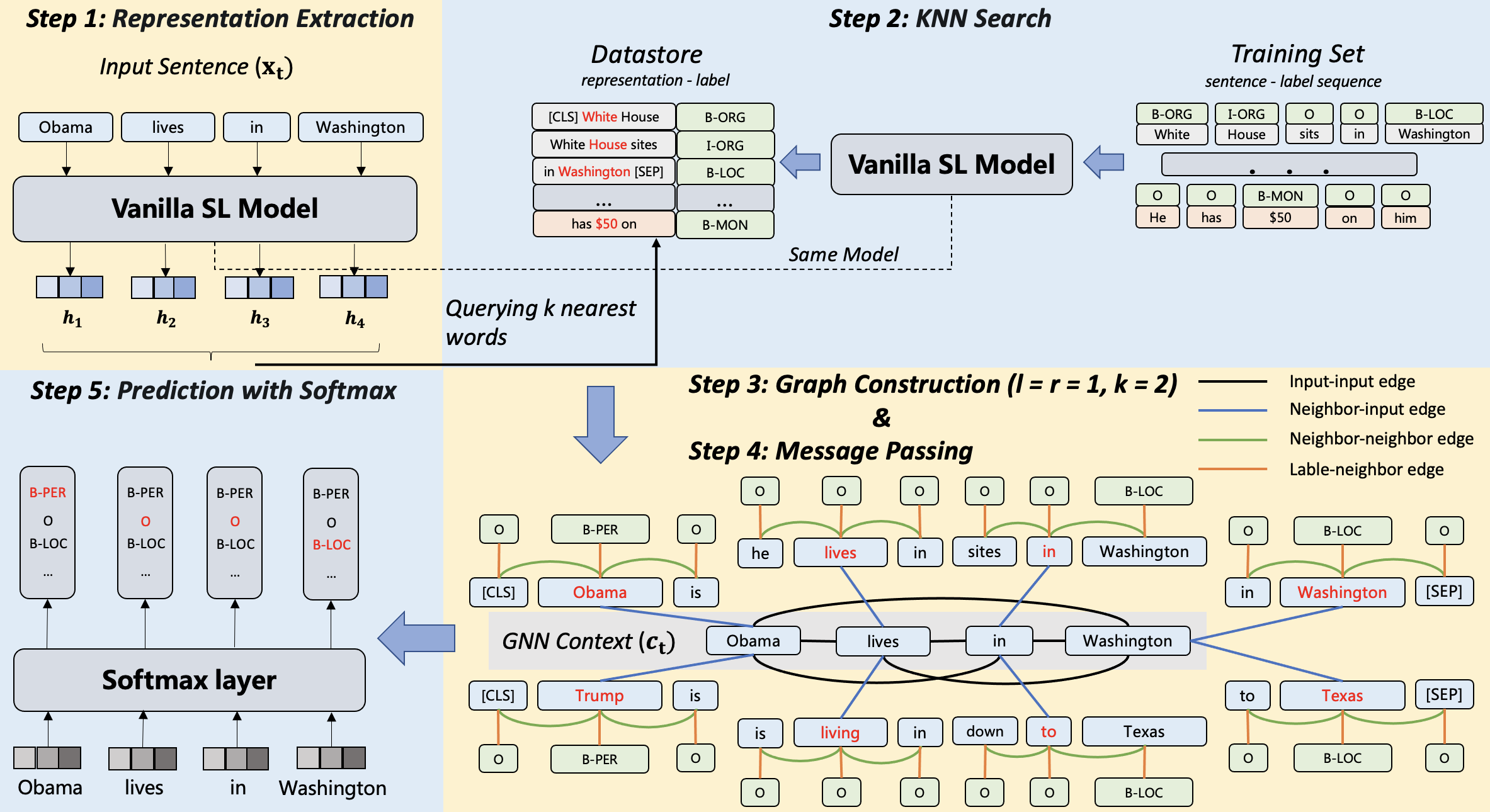
The proposed GNN-SL can be decomposed into five steps: (1) obtaining token features using a pre-trained vanilla sequence labeling model, which is the same as in KNN-SL; (2) obtaining nearest neighbors from the whole training set for each input word; (3) constructing an undirected graph between each word within the sentence and its nearest neighbors; (4) obtaining aggregated word representations through messages passing along the graph; and (5) feeding the aggregated word representation to the softmax layer to obtain the final label. The full pipeline is shown in Figure 2.
For steps (1) and (2), they are akin the strategies taken in KNN-SL. We will describe the details for steps (3) and (4) in order below.
4.2 Graph Construction
We formulate the graph as , where represents a collection of nodes and represents a collection of edges . refers to node types and refers to edge types.
Nodes
In the constructed graph, we define three types of nodes :
(1) Input nodes, denoted by , which correspond to words of the input sentence. In the example of Figure 2 Step 3, the input nodes are displayed with the word sequence ;
(2) Neighbor nodes, denoted by , which correspond to words in the retrieved neighbors. The context of nearest neighbors is also included (and thus treated as neighbor nodes) in an attempt to capture more abundant contextual information for the retrieved neighbors. For the example in Figure 2, for each input word with representation , nearest neighbors are queried from the cached representations of all words in the training set with the distance as the metric of similarity. Taking the input word as the example with , we obtain two nearest neighbors leveraging the NN search. The contexts of each retrieved nearest neighbor are also considered by adding both left and right contexts around the retrieved nearest neighbor, where is expanded to and is expanded to 222[CLS] is a special token usually applied in pre-training language models (e.g., BERT) representing the beginning of a sentence.. The analysis of the size of the context is conducted in Section 6.
(3) Label nodes, denoted by , since the labels of nearest neighbors provide important evidence for the input node to classify, we wish to pass the influence of neighbors’ labels to the input node along the graph. As will be shown in ablation studies in Section 6, the consideration of label nodes introduces a significant performance boost. Shown in Figure 2 Step 3, taking the input word as the example, the two retrieved nearest neighbors are and , and both the corresponding node labels are .
With the above formulated, can be rewritten as .
Edges
Given the three types of nodes , we connect them using different types of edges to enable information passing.
We define four types of edges for : (1) edges within the input nodes , notated by ; (2) edges between the neighbor nodes and the input nodes , notated by ; (3) edges within the neighbor nodes , notated by ; and (4) edges between the label nodes and the neighbor nodes , denoted by . All types of edges are bi-directional which allows information passing on both sides. We use different colors to differentiate different relations in Figure 2 Step 3.
For and , they respectively mimic the attention mechanism to aggregate the context information within the input word sequence or the expanded nearest context, which are shown with the black and green color in Figure 2. For , it connects the retrieved neighbors and the query input word, transferring the neighbor information to the input word. For colored with orange, information is passed from label nodes to neighbor nodes, which is ultimately transferred to input nodes.
4.3 Message Passing On The Graph
Given the constructed graph, we next use graph neural networks (GNNs) to aggregate information based on the graph to obtain the final representation for each token to classify. More formally, we define the l-th layer representation of node as follows:
| (4) |
where denotes the information transferred from the node to the node along the edge , denotes the edge weight modeling the importance of the source node on the target node with the relationship , and denotes the function to aggregate the transferred information from the neighbors of node . We detail how to obtain A(), M(), and Aggregate() below.
Message
For each edge , the message transferred from the source node to the target node can be formulated as:
| (5) |
where denotes the dimensionality of the vector, and are two learnable weight matrixes controling the outflow of node from the node side and the edge side respectively.
For the receiver node , the importance of each neighbor with the relationship can be viewed as the attention mechanism in Vaswani et al. (2017), which relates different positions of a single sequence. To introduce the attention weights, we first map the source node to a key vector and the target node to a query vector :
| (6) |
where and are two learnable matrixes.
As we use different types of edges for node connections, we follow Hu et al. (2020) to keep a distinct edge-matrix for each edge type between the dot of and :
| (7) | ||||
where is a learnable matrix denoting the contribution of each edge with a different relationship. Similar to Vaswani et al. (2017), the final attention is the concatenation of heads which compute the attention weights independently:
| (8) | ||||
where is the number of heads for multi-head attention (8 is used for our model) and is a learnable model parameter.
Aggregate
For each edge , we now have the attention weight and the information , the next step is to obtain the weighted-sum information from all neighboring nodes:
| (9) |
where is element-wise addition and is a learnable model parameter used as an activation function like a linear layer.
The aggregated representation for each input word is used as its final representation, passed to the softmax layer for classification. For all our experiments, the number of heads is 8.
| English CoNLL 2003 | |||
| Model | Precision | Recall | F1 |
| CVT (Clark et al., 2018) | - | - | 92.22 |
| BERT-MRC (Li et al., 2019a) | 92.33 | 94.61 | 93.04 |
| BERT-Large (Devlin et al., 2018) | - | - | 92.8 |
| BERT-Large+KNN | 92.90 | 92.88 | 92.86 (+0.06) |
| BERT-Large+GNN | 92.92 | 93.34 | 93.14 (+0.33) |
| BERT-Large+GNN+KNN | 92.95 | 93.37 | 93.16 (+0.35) |
| RoBERTa-Large (Liu et al., 2019) | 92.77 | 92.81 | 92.76 |
| RoBERTa-Large+KNN | 92.82 | 92.99 | 92.93 (+0.17) |
| RoBERTa-Large+GNN | 93.00 | 93.41 | 93.20 (+0.44) |
| RoBERTa-Large+GNN+KNN | 93.02 | 93.40 | 93.20 (+0.44) |
| English OntoNotes 5.0 | |||
| Model | Precision | Recall | F1 |
| CVT (Clark et al., 2018) | - | - | 88.8 |
| BERT-MRC (Li et al., 2019a) | 92.98 | 89.95 | 91.11 |
| BERT-Large (Devlin et al., 2018) | 90.01 | 88.35 | 89.16 |
| BERT-Large+KNN | 89.93 | 91.65 | 90.78 (+1.62) |
| BERT-Large+GNN | 91.44 | 91.16 | 91.30 (+2.14) |
| BERT-Large+GNN+KNN | 91.47 | 91.14 | 91.32 (+2.16) |
| RoBERTa-Large (Liu et al., 2019) | 89.77 | 89.27 | 89.52 |
| RoBERTa-Large+KNN | 90.00 | 91.26 | 90.63 (+1.11) |
| RoBERTa-Large+GNN | 91.38 | 91.17 | 91.30 (+1.78) |
| RoBERTa-Large+GNN+KNN | 91.48 | 91.29 | 91.39 (+1.87) |
| Chinese OntoNotes 4.0 | |||
| Model | Precision | Recall | F1 |
| Lattice-LSTM (Zhang and Yang, 2018) | 76.35 | 71.56 | 73.88 |
| Glyce-BERT (Meng et al., 2019) | 81.87 | 81.40 | 80.62 |
| BERT-MRC (Li et al., 2019a) | 82.98 | 81.25 | 82.11 |
| BERT-Large (Devlin et al., 2018) | 78.01 | 80.35 | 79.16 |
| BERT-Large+KNN | 80.23 | 81.60 | 80.91 (+1.75) |
| BERT-Large+GNN | 83.06 | 81.60 | 82.33 (+3.17) |
| BERT-Large+GNN+KNN | 83.07 | 81.62 | 82.35 (+3.19) |
| ChineseBERT-Large (Sun et al., 2021) | 80.77 | 83.65 | 82.18 |
| ChineseBERT-Large+KNN | 81.68 | 83.46 | 82.56 (+0.38) |
| ChineseBERT-Large+GNN | 82.02 | 84.01 | 83.02 (+0.84) |
| ChineseBERT-Large+GNN+KNN | 82.21 | 83.98 | 83.10 (+0.92) |
| Chinese MSRA | |||
| Model | Precision | Recall | F1 |
| Lattice-LSTM (Zhang and Yang, 2018) | 93.57 | 92.79 | 93.18 |
| Glyce-BERT (Meng et al., 2019) | 95.57 | 95.51 | 95.54 |
| BERT-MRC (Li et al., 2019a) | 96.18 | 95.12 | 95.75 |
| BERT-Large (Devlin et al., 2018) | 94.97 | 94.62 | 94.80 |
| BERT-Large+KNN | 95.34 | 94.64 | 94.99 (+0.19) |
| BERT-Large+GNN | 96.29 | 95.51 | 95.90 (+1.10) |
| BERT-Large+GNN+KNN | 96.31 | 95.54 | 95.93 (+1.13) |
| ChineseBERT-Large (Sun et al., 2021) | 95.61 | 95.61 | 95.61 |
| ChineseBERT-Large+KNN | 95.83 | 95.68 | 95.76 (+0.15) |
| ChineseBERT-Large+GNN | 96.28 | 95.73 | 96.01 (+0.40) |
| ChineseBERT-Large+GNN+KNN | 96.29 | 95.75 | 96.03 (+0.42) |
| PKU | |||
| Model | Precision | Recall | F1 |
| Multitask pretrain (Yang et al., 2017) | - | - | 96.3 |
| CRF-LSTM (Huang et al., 2019) | - | - | 96.6 |
| Glyce-BERT (Meng et al., 2019) | 97.1 | 96.4 | 96.7 |
| BERT-Large (Devlin et al., 2018) | 96.8 | 96.3 | 96.5 |
| BERT-Large+KNN | 97.2 | 96.1 | 96.6 (+0.1) |
| BERT-Large+GNN | 96.9 | 96.6 | 96.8 (+0.3) |
| BERT-Large+GNN+KNN | 96.9 | 96.7 | 96.8 (+0.3) |
| ChineseBERT-Large (Sun et al., 2021) | 97.3 | 96.0 | 96.7 |
| ChineseBERT-Large+KNN | 97.3 | 96.1 | 96.7 (+0.0) |
| ChineseBERT-Large+GNN | 97.6 | 96.2 | 96.9 (+0.2) |
| ChineseBERT-Large+GNN+KNN | 97.7 | 96.2 | 96.9 (+0.2) |
| CITYU | |||
| Model | Precision | Recall | F1 |
| Multitask pretrain (Yang et al., 2017) | - | - | 96.9 |
| CRF-LSTM (Huang et al., 2019) | - | - | 97.6 |
| Glyce-BERT (Meng et al., 2019) | 97.9 | 98.0 | 97.9 |
| BERT-Large (Devlin et al., 2018) | 97.5 | 97.7 | 97.6 |
| BERT-Large+KNN | 97.8 | 97.8 | 97.8 (+0.2) |
| BERT-Large+GNN | 98.0 | 98.1 | 98.0 (+0.4) |
| BERT-Large+GNN+KNN | 98.0 | 98.1 | 98.0 (+0.4) |
| ChineseBERT-Large (Sun et al., 2021) | 97.8 | 98.2 | 98.0 |
| ChineseBERT-Large+KNN | 98.1 | 98.0 | 98.1 (+0.1) |
| ChineseBERT-Large+GNN | 98.2 | 98.4 | 98.3 (+0.3) |
| ChineseBERT-Large+GNN+KNN | 98.3 | 98.4 | 98.3 (+0.3) |
| MSR | |||
| Model | Precision | Recall | F1 |
| Multitask pretrain (Yang et al., 2017) | - | - | 97.5 |
| CRF-LSTM (Huang et al., 2019) | - | - | 97.9 |
| Glyce-BERT (Meng et al., 2019) | 98.2 | 98.3 | 98.3 |
| BERT-Large (Devlin et al., 2018) | 98.1 | 98.2 | 98.1 |
| BERT-Large+KNN | 98.3 | 98.4 | 98.3 (+0.2) |
| BERT-Large+GNN | 98.4 | 98.3 | 98.4 (+0.3) |
| BERT-Large+GNN+KNN | 98.4 | 98.3 | 98.4 (+0.3) |
| ChineseBERT-Large (Sun et al., 2021) | 98.5 | 98.0 | 98.3 |
| ChineseBERT-Large+KNN | 98.5 | 98.1 | 98.3 (+0.0) |
| ChineseBERT-Large+GNN | 98.9 | 97.9 | 98.5 (+0.2) |
| ChineseBERT-Large+GNN+KNN | 98.9 | 98.0 | 98.5 (+0.2) |
| AS | |||
| Model | Precision | Recall | F1 |
| Multitask pretrain (Yang et al., 2017) | - | - | 95.7 |
| CRF-LSTM (Huang et al., 2019) | - | - | 96.6 |
| Glyce-BERT (Meng et al., 2019) | 96.6 | 96.8 | 96.7 |
| BERT-Large (Devlin et al., 2018) | 96.7 | 96.4 | 96.5 |
| BERT-Large+KNN | 96.2 | 96.9 | 96.6 (+0.1) |
| BERT-Large+GNN | 96.6 | 97.0 | 96.8 (+0.3) |
| BERT-Large+GNN+KNN | 96.6 | 97.0 | 96.8 (+0.3) |
| ChineseBERT-Large (Sun et al., 2021) | 96.3 | 97.2 | 96.7 |
| ChineseBERT-Large+KNN | 96.3 | 97.2 | 96.7 (+0.0) |
| ChineseBERT-Large+GNN | 96.1 | 97.7 | 96.9 (+0.2) |
| ChineseBERT-Large+GNN+KNN | 96.2 | 97.7 | 96.9 (+0.2) |
| Chinese CTB5 | Chinese CTB6 | Chinese UD1.4 | |||||||
| Model | Precision | Recall | F1 | Precision | Recall | F1 | Precision | Recall | F1 |
| Joint-POS(Sig) (Shao et al., 2017) | 93.68 | 94.47 | 94.07 | - | - | 90.81 | 89.28 | 89.54 | 89.41 |
| Joint-POS(Ens) (Shao et al., 2017) | 93.95 | 94.81 | 94.38 | - | - | - | 89.67 | 89.86 | 89.75 |
| Lattice-LSTM (Zhang and Yang, 2018) | 94.77 | 95.51 | 95.14 | 92.00 | 90.86 | 91.43 | 90.47 | 89.70 | 90.09 |
| Glyce-BERT (Meng et al., 2019) | 96.50 | 96.74 | 96.61 | 95.56 | 95.26 | 95.41 | 96.19 | 96.10 | 96.14 |
| BERT-Large (Devlin et al., 2018) | 95.86 | 96.26 | 96.06 | 94.91 | 94.63 | 94.77 | 95.42 | 94.17 | 94.79 |
| BERT-Large+KNN | 96.36 | 96.60 | 96.48 (+0.42) | 95.14 | 94.77 | 94.95 (+0.18) | 95.85 | 95.67 | 95.76 (+0.97) |
| BERT-Large+GNN | 96.86 | 96.66 | 96.76 (+0.70) | 96.46 | 94.82 | 95.64 (+0.85) | 96.14 | 96.46 | 96.30 (+1.51) |
| BERT-Large+GNN+KNN | 96.77 | 96.69 | 96.79 (+0.73) | 96.44 | 94.84 | 95.64 (+0.85) | 96.20 | 96.47 | 96.34 (+1.55) |
| ChineseBERT (Sun et al., 2021) | 96.35 | 96.54 | 96.44 | 95.47 | 95.00 | 95.23 | 96.02 | 95.92 | 95.97 |
| ChineseBERT+KNN | 96.41 | 96.15 | 96.52 (+0.08) | 95.48 | 95.09 | 95.29 (+0.06) | 96.11 | 96.11 | 96.11 (+0.14) |
| ChineseBERT+GNN | 96.46 | 97.41 | 96.94 (+0.50) | 96.08 | 95.50 | 95.79 (+0.77) | 96.18 | 96.54 | 96.36 (+0.39) |
| ChineseBERT+GNN+KNN | 96.46 | 97.44 | 96.96 (+0.52) | 96.13 | 95.58 | 95.85 (+0.82) | 96.25 | 96.57 | 96.40 (+0.43) |
| English WSJ | |||
| Model | Precision | Recall | F1 |
| Meta BiLSTM (Bohnet et al., 2018) | - | - | 98.23 |
| BERT-Large (Devlin et al., 2018) | 99.21 | 98.36 | 98.86 |
| BERT-Large+KNN | 98.98 | 98.85 | 98.92 (+0.06) |
| BERT-Large+GNN | 98.84 | 98.98 | 98.94 (+0.08) |
| BERT-Large+GNN+KNN | 98.88 | 98.99 | 98.96 (+0.10) |
| RoBERTa-Large (Liu et al., 2019) | 99.22 | 98.44 | 98.90 |
| RoBERTa-Large+KNN | 99.21 | 98.52 | 98.94 (+0.04) |
| RoBERTa-Large+GNN | 98.90 | 99.06 | 99.00 (+0.10) |
| RoBERTa-Large+GNN+KNN | 98.90 | 99.06 | 99.00 (+0.10) |
| English Tweets | |||
| Model | Precision | Recall | F1 |
| FastText+CNN+CRF | - | - | 91.78 |
| BERT-Large (Devlin et al., 2018) | 92.33 | 91.98 | 92.34 |
| BERT-Large+KNN | 92.77 | 92.02 | 92.39 (+0.05) |
| BERT-Large+GNN | 92.38 | 92.52 | 92.45 (+0.11) |
| BERT-Large+GNN+KNN | 92.42 | 92.53 | 92.48 (+0.14) |
| RoBERTa-Large (Liu et al., 2019) | 92.40 | 91.99 | 92.38 |
| RoBERTa-Large+KNN | 92.44 | 92.11 | 92.46 (+0.08) |
| RoBERTa-Large+GNN | 92.49 | 92.53 | 92.51 (+0.13) |
| RoBERTa-Large+GNN+KNN | 92.49 | 92.54 | 92.52 (+0.14) |
5 Experiments
We conduct experiments on three widely-used sub-tasks of sequence labeling: named entity recognition (NER), part of speech tagging (POS), and Chinese Word Segmentation (CWS).
5.1 Trainng Details
The Vanilla SL Model
As described in Section 4, we need the pre-trained vanilla SL model to extract features to initial the nodes of the constructed graph. For all our experiments, we choose the standard BERT-large Devlin et al. (2018) and RoBERTa-large Liu et al. (2019) for English tasks, as well as the standard BERT-large and ChineseBERT-large Sun et al. (2021) for Chinese tasks.
NN Retrieval
In the process of NN retrieval, the number of nearest neighbors is set to 32, and the size of the nearest context window is set to 7 (setting both the left and right side of the window to 3). The two numbers are chosen according to the evaluation in Section 6 and perform best in our experiments. For the nearest search, we use the last layer output of the pre-trained vanilla SL model as the representation and the distance as the metric of similarity comparison.
5.2 Control Experiments
To better show the effectiveness of the proposed model, we compare the performance of the following setups: (1) vanilla SL models: vanilla models naturally constitute a baseline for comparison, where the final layer representation is fed to a softmax function to obtain for label prediction; (2) vanilla + NN: the NN probability is interpolated with to obtain final predictions; (3) vanilla + GNN: the representation generated from the final layer of GNN is passed to the softmax layer to obtain the label probability ; (4) vanilla + GNN + NN: the NN probability is interpolated with the GNN probability to obtain final predictions, rather than the probability from the vanilla model, as in vanilla + NN.
| Input Sentence #1 | |
| Hornak moved on from Tigers to Phoenix for studies and work. | |
| Ground Truth: ORGANIZATION, Vanilla SL Output: LOCATION, GNN-SL Output: ORGANIZATION | |
| Retrieved Nearest Neighbors | Retrieved Label |
| 1-th: Hornak signed accomplished performance in a Tigers display against Phoenix. | ORGANIZATION |
| 8-th: Blinker was fined 75,000 Swiss francs ($57,600) for failing to inform the English club of his previous commitment to Udinese. | ORGANIZATION |
| 16-th: Since we have friends in Phoenix, we pop in there for a brief visit. | LOCATION |
| Input Sentence #2 | |
| Australian Tom Moody took six for 82 but Tim O’Gorman, 109, took Derbyshire to 471. | |
| Ground Truth: PERSON, Vanilla SL Output: - (Not an Entity), GNN-SL Output: PERSON | |
| Retrieved Nearest Neighbors | Retrieved Label |
| 1-th: At California, Troy O’Leary hit solo home runs in the second inning as the surging Boston Red Sox. | PERSON |
| 8-th: Britain’s Chris Boardman broke the world 4,000 meters cycling record by more than six seconds. | PERSON |
| 16-th: Japan coach Shu Kamo said: The Syrian own goal proved lucky for us. | PERSON |
5.3 Named Entity Recognition
Details
Results
Results for the NER task are shown in Table 1, and from the results:
(1) We observe a significant performance boost brought by NN, respectively +0.06, +1.62, +1.75 and +0.19 for English CoNLL 2003, English OntoNotes 5.0, Chinese OntoNotes 4.0 and Chinese MSRA. which proves the importance of incorporating the evidence of retrieved neighbors.
(2) We observe a significant performance boost for vanilla+GNN over both the vanilla model: respectively +2.14 on the BERT-Large and +1.78 on the RoBERTa-Large for English OntoNotes 5.0, and +1.10 on the BERT-Large and +0.40 on the ChineseBERT-Large for Chinese MSRA. Due to the fact that both vanilla+GNN and the vanilla model output the final layer representation to the softmax function to obtain final probability and that do not participate in the final probability interpolation for both, the performance boost over vanilla SL demonstrates that we are able to obtain better token-level representations using GNNs.
(3) When comparing with vanilla+NN, we observe further improvements of +0.33, +2.14, +3.17 and +1.10 for English CoNLL 2003, English OntoNotes 5.0, Chinese OntoNotes 4.0 and Chinese MSRA dataset, respectively, showing that the proposed GNN model has the ability to filtrate the useful neighbors to augment the vanilla SL model;
(4) There is an inconspicuous improvement brought by interpolating both the NN probability and GNN probability (vanilla + NN + GNN) over the proposed GNN-SL (vanilla + GNN), e.g., +2.16 v.s. +2.14 on the BERT-Large for English OntoNotes 5.0, and +1.13 v.s. +1.10 on the BERT-Large for Chinese MSRA. This demonstrates that as the evidence of retrieved nearest neighbors (and their labels) has been assimilated through GNNs in the representation learning stage, the extra benefits brought by interpolating in the final prediction stage is significantly narrowed.
5.4 Chinese Word Segmentation
Details
The task of CWS is normally treated as a char-level tagging problem: assigning seg or not seg for each input word.
For evaluation, four Chinese datasets retrieved from SIGHAN 2005333The website of the 4-th Second International Chinese Word Segmentation Bakeoff (SIGHAN 2005) is: http://sighan.cs.uchicago.edu/bakeoff2005/ are used: PKU, MSR, CITYU, and AS, and benchmarks Multitask pretrain Yang et al. (2017), CRF-LSTM Huang et al. (2019) and Glyce+BERT Meng et al. (2019) are chosen for the comparison.
Results
Results for the CWS task are shown in Table 2. From the results, same as the former Section 5.3, with different vanilla models as the backbone, we can observe obvious improvements by applying the NN probability (vanilla + NN) or the GNN model (vanilla + GNN), while keeping the same results between vanilla + GNN and vanilla + GNN + NN, e.g., for PKU dataset +0.1 on BERT + NN, +0.3 both on BERT + GNN and BERT + GNN + NN. Notablely we achieve SOTA for all four datasets with the ChineseBERT: 96.9 (+0.2) on PKU, 98.3 (+0.3) on CITYU, 98.5 (+0.2) on MSR and 96.9 (+0.2) on AS.
5.5 Part of Speech Tagging
Details
The task of POS is normally formalized as a character-level sequence labeling task, assigning labels to each of the input word.
Results
Results for the POS task are shown in Table 3 for Chinese datasets and Table 4 for English datasets. As shown, with different vanilla models and datasets, the phenomenons are the same as the former Section 5.3 that improves largely based on the NN probability and further on the GNN model. For the results of Chinese CTB5 as the example, +0.42 on BERT + NN, further +0.70 on BERT + GNN, and +0.73 on BERT + GNN + NN.
Examples
To illustrate the augment of our proposed GNN-SL, we visualize the retrieved NN examples as well as the input sentence in Table 5. For the first example the long-tail case “Phoenix”, which is assigned with “LOCATION” by the vanilla SL model, is amended to “ORGANIZATION” by the nearest neighbors. Especially, we can observe that both 1-th and 8-th retrieved labels are “ORGANIZATION” while the 16-th retrieved label is “LOCATION” which is against the ground truth. That phenomenon proves that retrieved neighbors do relate to the input sentence in different ways: some are close to the original input sentence while others are just noise, and our proposed GNN-SL has the ability to better model the relationships between the retrieved nearest examples and the input word. For the second example, with the augment of the retrieved nearest neighbors, our proposed GNN-SL outputs the correct label “PERSON” for the word “Tom Moody”.
| Task NER | ||||||||||||
| English CoNLL 2003 | English OntoNotes 5.0 | Chinese OntoNotes 4.0 | Chinese MSRA | |||||||||
| Model | Precision | Recall | F1 | Precision | Recall | F1 | Precision | Recall | F1 | Precision | Recall | F1 |
| BERT+GNN | 92.97 | 93.37 | 93.17 | 91.40 | 91.15 | 91.27 | 83.04 | 81.56 | 82.30 | 96.69 | 95.51 | 95.90 |
| BERT+GNN-without Label nodes | 92.99 | 93.29 | 93.14 (-0.03) | 91.66 | 90.70 | 91.18 (-0.09) | 83.23 | 81.06 | 82.13 (-0.17) | 95.86 | 95.31 | 95.58 (-0.32) |
| Task CWS | ||||||||||||
| PKU | CITYU | MSR | AS | |||||||||
| Model | Precision | Recall | F1 | Precision | Recall | F1 | Precision | Recall | F1 | Precision | Recall | F1 |
| BERT+GNN | 96.9 | 96.6 | 96.8 | 98.0 | 98.1 | 98.0 | 98.4 | 98.3 | 98.4 | 96.6 | 97.0 | 96.8 |
| BERT+GNN-without Label nodes | 97.1 | 96.2 | 96.7 (-0.1) | 97.9 | 97.8 | 97.9 (-0.1) | 98.4 | 98.2 | 98.3 (-0.1) | 96.3 | 97.1 | 96.7 (-0.1) |
| Task POS | ||||||||||||
| Chinese CTB5 | Chinese CTB6 | Chinese UD1.4 | English WSJ | |||||||||
| Model | Precision | Recall | F1 | Precision | Recall | F1 | Precision | Recall | F1 | Precision | Recall | F1 |
| BERT+GNN | 96.87 | 96.69 | 96.78 | 96.44 | 94.82 | 95.63 | 96.15 | 96.47 | 96.31 | 98.85 | 98.99 | 98.95 |
| BERT+GNN-without Label nodes | 96.36 | 96.58 | 96.46 (-0.32) | 95.69 | 94.69 | 95.19 (-0.42) | 95.99 | 96.05 | 96.02 (-0.29) | 98.97 | 98.87 | 98.92 (-0.003) |

| F1-score on English OntoNotes 5.0 | |
| Context (l+r+1) / Model | F1-score |
| The Vanilla SL Model | 89.16 |
| GNN-SL | |
| + by setting context=3 | 91.16 (+2.00) |
| + by setting context=5 | 91.24 (+2.08) |
| + by setting context=7 | 91.27 (+2.11) |
| + by setting context=9 | 91.27 (+2.11) |
| + by setting context=11 | 91.27 (+2.11) |
6 Ablation Study
6.1 The Number of Retrieved Neighbors
To evaluate the influence of the amount of the retrieved information from the training set, we conduct experiments on English OntoNotes 5.0 for the NER task by varying the number of neighbors . The results are shown in Figure 3. As can be seen, as increases, the F1 score of GNN-SL first increases and then decreases. The explanation is as follows, as more examples are, more noise is introduced and relevance to the query decreases, which makes performance worse.
6.2 Effectiveness of Label Nodes
In Section 4.2, labels are used as nodes in the graph construction process, where their influence can be propagated to the input nodes through and . To evaluate the effectiveness of that strategy, we conducted contrast experiments by removing the label nodes. The experiments are based on the BERT-Large model and adjusted to the best parameters, and the results are shown in Table 6 for all three tasks. All the results show a decrease after removing the label nodes, especially -0.42 for the POS Chinese CTB6 dataset and -0.32 for the NER Chinese MSRA dataset, which proves the necessity of directly incorporating label information of neighbors in passing the message.
6.3 The Size of the Context Window
In Section 4.2, to acquire the context information of each retrieved nearest word we expand the retrieved nearest word to the nearest context. We experiment with varying context sizes to show the influence. Results on English OntoNotes 5.0 for the NER task are shown in Table 7. We can observe that, as the context size increases, performance first goes up and then plateaus. The explanation is as follows: a decent size of context is sufficient to provide enough information for predictions.
6.4 NN search without Fine-tuning
In section 4, we use the representations obtained by the fine-tuned pre-trained model on the labeled training set to perform NN search. To validate its necessity, we also conduct an experiment that directly uses the BERT model without fine-tuning to extract representation. We evaluate its influence on CoNLL 2003 for the NER task and observe a sharp decrease when switching the fine-tuned SL model to a non fine-tuned BERT model, i.e., 93.17 v.s. 92.83. The explanation is due to the gap between the language model task and the sequence labeling task, and that nearest neighbors retrieved by a vanilla pre-trained language model might not be the nearest neighbor for the SL task.
7 Conclusion
In this work, we propose graph neural networks sequence labeling (GNN-SL), which augments the vanilla SL model output with similar tagging examples retrieved from the whole training set. Since not all the retrieved tagging examples benefit the model prediction, we construct a heterogeneous graph, in which nodes represent the input words associating its nearest examples and edges represent the relationship between each node, and leverage graph neural networks (GNNs) to transfer information from the retrieved nearest tagging examples to the input word. This strategy enables the model to directly acquire similar tagging examples and improves the effectiveness in handling long-tail cases. We conduct multi experiments and analyses on three sequence labeling tasks: NER, POS, and CWS. Notably, GNN-SL achieves SOTA 96.9 (+0.2) on PKU, 98.3 (+0.4) on CITYU, 98.5 (+0.2) on MSR, and 96.9 (+0.2) on AS for the CWS task.
References
- Bohnet et al. (2018) Bernd Bohnet, Ryan McDonald, Goncalo Simoes, Daniel Andor, Emily Pitler, and Joshua Maynez. 2018. Morphosyntactic tagging with a meta-bilstm model over context sensitive token encodings. arXiv preprint arXiv:1805.08237.
- Chiu and Nichols (2016) Jason PC Chiu and Eric Nichols. 2016. Named entity recognition with bidirectional lstm-cnns. Transactions of the association for computational linguistics, 4:357–370.
- Clark et al. (2018) Kevin Clark, Minh-Thang Luong, Christopher D Manning, and Quoc V Le. 2018. Semi-supervised sequence modeling with cross-view training. arXiv preprint arXiv:1809.08370.
- Collobert et al. (2011) Ronan Collobert, Jason Weston, Léon Bottou, Michael Karlen, Koray Kavukcuoglu, and Pavel Kuksa. 2011. Natural language processing (almost) from scratch. Journal of machine learning research, 12(ARTICLE):2493–2537.
- Cui and Zhang (2019) Leyang Cui and Yue Zhang. 2019. Hierarchically-refined label attention network for sequence labeling. arXiv preprint arXiv:1908.08676.
- Dai et al. (2019) Dai Dai, Xinyan Xiao, Yajuan Lyu, Shan Dou, Qiaoqiao She, and Haifeng Wang. 2019. Joint extraction of entities and overlapping relations using position-attentive sequence labeling. In Proceedings of the AAAI conference on artificial intelligence, volume 33, pages 6300–6308.
- De Cao et al. (2018) Nicola De Cao, Wilker Aziz, and Ivan Titov. 2018. Question answering by reasoning across documents with graph convolutional networks. arXiv preprint arXiv:1808.09920.
- Devlin et al. (2018) Jacob Devlin, Ming-Wei Chang, Kenton Lee, and Kristina Toutanova. 2018. Bert: Pre-training of deep bidirectional transformers for language understanding. arXiv preprint arXiv:1810.04805.
- Fan et al. (2020) Angela Fan, Claire Gardent, Chloe Braud, and Antoine Bordes. 2020. Augmenting transformers with knn-based composite memory for dialogue. arXiv preprint arXiv:2004.12744.
- Gan et al. (2021) Leilei Gan, Yuxian Meng, Kun Kuang, Xiaofei Sun, Chun Fan, Fei Wu, and Jiwei Li. 2021. Dependency parsing as mrc-based span-span prediction. arXiv preprint arXiv:2105.07654.
- Guu et al. (2020) Kelvin Guu, Kenton Lee, Zora Tung, Panupong Pasupat, and Ming-Wei Chang. 2020. Realm: Retrieval-augmented language model pre-training. arXiv preprint arXiv:2002.08909.
- Hamilton et al. (2017) Will Hamilton, Zhitao Ying, and Jure Leskovec. 2017. Inductive representation learning on large graphs. Advances in neural information processing systems, 30.
- Hammerton (2003) James Hammerton. 2003. Named entity recognition with long short-term memory. In Proceedings of the seventh conference on Natural language learning at HLT-NAACL 2003, pages 172–175.
- Hu et al. (2020) Ziniu Hu, Yuxiao Dong, Kuansan Wang, and Yizhou Sun. 2020. Heterogeneous graph transformer. pages 2704–2710.
- Huang et al. (2019) Weipeng Huang, Xingyi Cheng, Kunlong Chen, Taifeng Wang, and Wei Chu. 2019. Toward fast and accurate neural chinese word segmentation with multi-criteria learning. arXiv preprint arXiv:1903.04190.
- Karpukhin et al. (2020) Vladimir Karpukhin, Barlas Oğuz, Sewon Min, Patrick Lewis, Ledell Wu, Sergey Edunov, Danqi Chen, and Wen-tau Yih. 2020. Dense passage retrieval for open-domain question answering. arXiv preprint arXiv:2004.04906.
- Khandelwal et al. (2020) Urvashi Khandelwal, Angela Fan, Dan Jurafsky, Luke Zettlemoyer, and Mike Lewis. 2020. Nearest neighbor machine translation. arXiv preprint arXiv:2010.00710.
- Khandelwal et al. (2019) Urvashi Khandelwal, Omer Levy, Dan Jurafsky, Luke Zettlemoyer, and Mike Lewis. 2019. Generalization through memorization: Nearest neighbor language models. arXiv preprint arXiv:1911.00172.
- Lample et al. (2016) Guillaume Lample, Miguel Ballesteros, Sandeep Subramanian, Kazuya Kawakami, and Chris Dyer. 2016. Neural architectures for named entity recognition. arXiv preprint arXiv:1603.01360.
- Levow (2006) Gina-Anne Levow. 2006. The third international Chinese language processing bakeoff: Word segmentation and named entity recognition. In Proceedings of the Fifth SIGHAN Workshop on Chinese Language Processing, pages 108–117, Sydney, Australia. Association for Computational Linguistics.
- Lewis et al. (2020) Mike Lewis, Marjan Ghazvininejad, Gargi Ghosh, Armen Aghajanyan, Sida Wang, and Luke Zettlemoyer. 2020. Pre-training via paraphrasing. arXiv preprint arXiv:2006.15020.
- Li et al. (2019a) Xiaoya Li, Jingrong Feng, Yuxian Meng, Qinghong Han, Fei Wu, and Jiwei Li. 2019a. A unified mrc framework for named entity recognition. arXiv preprint arXiv:1910.11476.
- Li et al. (2019b) Xiaoya Li, Xiaofei Sun, Yuxian Meng, Junjun Liang, Fei Wu, and Jiwei Li. 2019b. Dice loss for data-imbalanced nlp tasks. arXiv preprint arXiv:1911.02855.
- Lin et al. (2021) Jerry Chun-Wei Lin, Yinan Shao, Youcef Djenouri, and Unil Yun. 2021. Asrnn: a recurrent neural network with an attention model for sequence labeling. Knowledge-Based Systems, 212:106548.
- Lin et al. (2020) Jerry Chun-Wei Lin, Yinan Shao, Ji Zhang, and Unil Yun. 2020. Enhanced sequence labeling based on latent variable conditional random fields. Neurocomputing, 403:431–440.
- Liu et al. (2018a) Liyuan Liu, Jingbo Shang, Xiang Ren, Frank Xu, Huan Gui, Jian Peng, and Jiawei Han. 2018a. Empower sequence labeling with task-aware neural language model. In Proceedings of the AAAI Conference on Artificial Intelligence, volume 32.
- Liu et al. (2019) Yinhan Liu, Myle Ott, Naman Goyal, Jingfei Du, Mandar Joshi, Danqi Chen, Omer Levy, Mike Lewis, Luke Zettlemoyer, and Veselin Stoyanov. 2019. Roberta: A robustly optimized bert pretraining approach. arXiv preprint arXiv:1907.11692.
- Liu et al. (2018b) Ziqi Liu, Chaochao Chen, Xinxing Yang, Jun Zhou, Xiaolong Li, and Le Song. 2018b. Heterogeneous graph neural networks for malicious account detection. pages 2077–2085.
- Ma and Hovy (2016) Xuezhe Ma and Eduard Hovy. 2016. End-to-end sequence labeling via bi-directional lstm-cnns-crf. arXiv preprint arXiv:1603.01354.
- Meng et al. (2021a) Yuxian Meng, Xiaoya Li, Xiayu Zheng, Fei Wu, Xiaofei Sun, Tianwei Zhang, and Jiwei Li. 2021a. Fast nearest neighbor machine translation. arXiv preprint arXiv:2105.14528.
- Meng et al. (2019) Yuxian Meng, Wei Wu, Fei Wang, Xiaoya Li, Ping Nie, Fan Yin, Muyu Li, Qinghong Han, Xiaofei Sun, and Jiwei Li. 2019. Glyce: Glyph-vectors for chinese character representations. Advances in Neural Information Processing Systems, 32.
- Meng et al. (2021b) Yuxian Meng, Shi Zong, Xiaoya Li, Xiaofei Sun, Tianwei Zhang, Fei Wu, and Jiwei Li. 2021b. Gnn-lm: Language modeling based on global contexts via gnn. arXiv preprint arXiv:2110.08743.
- Pradhan (2011) Sameer Pradhan. 2011. Proceedings of the fifteenth conference on computational natural language learning: Shared task. In Proceedings of the Fifteenth Conference on Computational Natural Language Learning: Shared Task.
- Pradhan et al. (2013) Sameer Pradhan, Alessandro Moschitti, Nianwen Xue, Hwee Tou Ng, Anders Björkelund, Olga Uryupina, Yuchen Zhang, and Zhi Zhong. 2013. Towards robust linguistic analysis using ontonotes. In Proceedings of the Seventeenth Conference on Computational Natural Language Learning, pages 143–152.
- Ritter et al. (2011) Alan Ritter, Sam Clark, Mausam, and Oren Etzioni. 2011. Named entity recognition in tweets: An experimental study. pages 1524–1534.
- Sang and De Meulder (2003) Erik F Sang and Fien De Meulder. 2003. Introduction to the conll-2003 shared task: Language-independent named entity recognition. arXiv preprint cs/0306050.
- Shao et al. (2017) Yan Shao, Christian Hardmeier, Jörg Tiedemann, and Joakim Nivre. 2017. Character-based joint segmentation and pos tagging for chinese using bidirectional rnn-crf. arXiv preprint arXiv:1704.01314.
- Shao et al. (2021) Yinan Shao, Jerry Chun-Wei Lin, Gautam Srivastava, Alireza Jolfaei, Dongdong Guo, and Yi Hu. 2021. Self-attention-based conditional random fields latent variables model for sequence labeling. Pattern Recognition Letters, 145:157–164.
- Song et al. (2018) Linfeng Song, Zhiguo Wang, Mo Yu, Yue Zhang, Radu Florian, and Daniel Gildea. 2018. Exploring graph-structured passage representation for multi-hop reading comprehension with graph neural networks. arXiv preprint arXiv:1809.02040.
- Sun et al. (2021) Zijun Sun, Xiaoya Li, Xiaofei Sun, Yuxian Meng, Xiang Ao, Qing He, Fei Wu, and Jiwei Li. 2021. Chinesebert: Chinese pretraining enhanced by glyph and pinyin information. arXiv preprint arXiv:2106.16038.
- Thulke et al. (2021) David Thulke, Nico Daheim, Christian Dugast, and Hermann Ney. 2021. Efficient retrieval augmented generation from unstructured knowledge for task-oriented dialog. arXiv preprint arXiv:2102.04643.
- Vaswani et al. (2017) Ashish Vaswani, Noam Shazeer, Niki Parmar, Jakob Uszkoreit, Llion Jones, Aidan N Gomez, Łukasz Kaiser, and Illia Polosukhin. 2017. Attention is all you need. Advances in neural information processing systems, 30.
- Veličković et al. (2017) Petar Veličković, Guillem Cucurull, Arantxa Casanova, Adriana Romero, Pietro Lio, and Yoshua Bengio. 2017. Graph attention networks. arXiv preprint arXiv:1710.10903.
- Vert et al. (2004) Jean-Philippe Vert, Koji Tsuda, and Bernhard Schölkopf. 2004. A primer on kernel methods. Kernel methods in computational biology, 47:35–70.
- Wang et al. (2020) Jiuniu Wang, Wenjia Xu, Xingyu Fu, Guangluan Xu, and Yirong Wu. 2020. Astral: adversarial trained lstm-cnn for named entity recognition. Knowledge-Based Systems.
- Wang et al. (2021) Shuhe Wang, Jiwei Li, Yuxian Meng, Rongbin Ouyang, Guoyin Wang, Xiaoya Li, Tianwei Zhang, and Shi Zong. 2021. Faster nearest neighbor machine translation. arXiv preprint arXiv:2112.08152.
- Xiong et al. (2020) Lee Xiong, Chenyan Xiong, Ye Li, Kwok-Fung Tang, Jialin Liu, Paul Bennett, Junaid Ahmed, and Arnold Overwijk. 2020. Approximate nearest neighbor negative contrastive learning for dense text retrieval. arXiv preprint arXiv:2007.00808.
- Xue et al. (2005) Naiwen Xue, Fei Xia, Fu-Dong Chiou, and Marta Palmer. 2005. The penn chinese treebank: Phrase structure annotation of a large corpus. Natural language engineering, 11(2):207–238.
- Yang et al. (2017) Jie Yang, Yue Zhang, and Fei Dong. 2017. Neural word segmentation with rich pretraining. arXiv preprint arXiv:1704.08960.
- Yao et al. (2019) Liang Yao, Chengsheng Mao, and Yuan Luo. 2019. Graph convolutional networks for text classification. 33(01):7370–7377.
- Yih (2020) Scott Yih. 2020. Retrieval-augmented generation for knowledge-intensive nlp tasks.
- Zhang and Yang (2018) Yue Zhang and Jie Yang. 2018. Chinese ner using lattice lstm. arXiv preprint arXiv:1805.02023.