Global solutions and blow-up for the wave equation with variable coefficients: II. boundary supercritical source
Abstract.
In this paper, we consider the wave equation with variable coefficients and boundary damping and supercritical source terms. The goal of this work is devoted to prove the local and global existence, and classify decay rate of energy depending on the growth near zero on the damping term. Moreover, we prove the blow-up of the weak solution with positive initial energy as well as nonpositive initial energy.
Key words and phrases:
wave equation with variable coefficients; supercritical source; existence of solutions; energy decay rates; blow-up2020 Mathematics Subject Classification:
35L05; 35L20; 35A01; 35B40; 35B441. Introduction
In this paper, we are concerned with the local and global existence, energy decay rates and finite time blow-up of the solution for the following wave equation
| (1.1) |
where , where is a symmetric and positive matrix, and , where is the outward unit normal to . is a bounded domain of () with smooth boundary . Here, and are closed and disjoint with .
During the past decades, the problem (1.1) has been widely studied. The condition means that represents an attractive force. When as in the present case, represents a source term. This situation is more delicate than attractive force, since the solution of (1.1) can blow up. The damping-source interplay in system (1.1) arise naturally in many contexts, for instance, in classical mechanics, fluid dynamics and quantum field theory (cf. [29, 41]). The interaction between two competitive force, that is damping term and source term, make the problem attractive from the mathematical point of view.
For the present case when is polynomial nonlinear source term such as , the stability of (1.1) has been studied by many authors (see [7, 8, 14, 15, 16, 17, 18, 20, 21, 22, 24, 25, 26, 27, 28, 30, 31, 36, 37, 38, 39, 43] and a list on references therein), where is subcritical or critical source. However, very few results addressed wave equations influenced by supercritical sources (cf. [1, 3, 11, 12, 42]). For example, [42] proved the local and global existence, uniqueness and Hadamard well-posedness for the wave equation when source terms can be supercritical or super-supercritical. However, the author do not considered the energy decay and blow-up of the solutions. [11] considered a system of nonlinear wave equations with supercritical sources and damping terms. They proved global existence and exponential and algebraic uniform decay rates of energy, moreover, blow-up result for weak solutions with nonnegative initial energy. But as far as I know, the only problem with considering supercritical source is the constant coefficients case, that is, and dimension .
In the case of variable coefficients, that is , boundary stability of the wave equation was considered in [4, 9, 15, 18, 22]. The wave equations with variable coefficients arise in mathematical modeling of inhomogeneous media in solid mechanics, electromagnetic, fluid flows through porous media. For the variable coefficients problem, the main tool is Riemannian geometry method, which was introduced by [46] and has been widely used in the literature, see [6, 9, 32, 33, 34, 44, 45] and a list of references therein. However, there were very few results considered the source term. For example, [4] proved the uniform decay rate of the energy to the viscoelastic wave equation with variable coefficients and acoustic boundary conditions without damping term. Recently, [26] studied the general decay rate of the energy for the wave equation with variable coefficients and Balakrishnan-Taylor damping and source term without imposing any restrictive growth near zero on the damping term. However, above mentioned examples were not considered Riemannian geometry, and only treated a subcritical source. More recently, [19] proved the uniform energy decay rates of the wave equation with variable coefficients applying the Riemannian geometry method and modified multiplier method. But, it was considered a subcritical source. [23] studied local and global existence, energy decay rate and blow-up of solution for the wave equation with variable coefficients, however it was not considered Reimannian geometry, and was treated the interior supercritical source. There is none, to my knowledge, for the variable coefficients problem having both damping and source terms on Riemannian geometry as well as considering boundary supercritical source.
Our main motivation is constituted by three dimensional case, in which the source term can be supercritical on variable coefficient problem. The differences from previous literatures are as follows:
-
(i)
Supercritical source for .
-
(ii)
Variable coefficient problem having source term on Riemannian geometry.
-
(iii)
Blow-up result with positive initial energy as well as nonpositive initial energy.
In order to overcome difficulties to prove above statements, first, we refine the energy space and a constant used in potential well method, because we do not guarantee since the source term is supercritical. Also we have a hypothesis on damping term for proving existence of solutions and energy decay rates (see Remark 2.2). Second, we use the Faedo-Galerkin method because nonlinear semigroup arguments considered in the previous literatures cannot be used since this paper deal with an operator , which depends on . Third, we refine the key point constants used to prove blow-up result. So, this paper has improved and generalized previous literatures.
The goal of this paper is to prove the existence result using the Faedo-Galerkin method and truncated approximation method, and classify the energy decay rate applying the method developed in [46] and [35]. Moreover, we prove the blow-up of the weak solution with positive initial energy as well as nonpositive initial energy. This paper is organized as follows: In Section 2, we recall the notation, hypotheses and some necessary preliminaries and introduce our main result. In Section 3, we prove the local existence of weak solutions, and show the global existence of weak solution in each two conditions in Section 4. In Section 5, we prove the uniform decay rate under suitable conditions on the initial data and boundary damping by the differential geometric approach. In Section 6, we prove the blow-up of the weak solution with positive initial energy as well as nonpositive initial energy. by using contradiction method.
2. Preliminaries
We begin this section by introducing some notations and our main results. Throughout this paper, we define the Hilbert space with the norm and with the norm . and are denoted by the norm and the norm, respectively, and and . Moreover, we need some notations on Riemannian geometry, it is mentioned in [46] and reference therein. For the reader’s comprehension, we will repeat them here.
Let be a symmetric and positive definite matrix for all and be smooth functions on satisfying
| (2.1) |
where is a positive constants. Set
For each , we define the inner product and the norm on the tangent space by
| (2.2) |
Then is a Riemannian manifold with Riemann metric . and are denoted by the gradient of u and Levi-Civita connection in the Riemannian metric , respectively. It follows that
| (2.3) |
Let be a vector field on . Then the covariant differential of determines a bilinear form on , for each , by
| (2.4) |
where is the covariant derivative of the vector field with respect to .
Hypothesis on .
Let be a bounded domain, , with smooth boundary . Here and are closed and disjoint with . There exists a vector field on the Riemannian manifold such that
| (2.5) |
where is a positive constant and
| (2.6) |
where represents the unit outward normal vector to . Moreover we assume that
| (2.7) |
Hypothesis on , .
Let satisfying following conditions:
| (2.8) |
where is a positive constant. We assume that
| (2.9) |
Hypothesis on .
Let be a nondecreasing function such that and suppose that there exist positive constants , , and a strictly increasing and odd function of class on such that
| (2.10) |
| (2.11) |
where denotes the inverse function of , and .
Hypothesis on .
Let be a constant satisfying the following condition:
| (2.12) |
Lemma 2.1.
([46]) Let and , be vector fields on . Then
-
(i)
-
(ii)
-
(iii)
-
(iv)
Remark 2.1.
Hypothesis (2.5) was introduced by Yao [46] for the exact controllability of the wave equation with variable coefficients. The existence of such a vector field depends on the sectional curvature of the Riemannian manifold . There are several methods and examples in [46] to find out a vector field that is satisfied the hypothesis (2.5). Specially, if , the constant coefficient case, the condition (2.5) is automatically satisfied by choosing for any .
Remark 2.2.
In view of the critical Sobolev imbedding , the map is not locally Lipschitz from into for the supercritical values . However, by the hypothesis on , is locally Lipschitz from into .
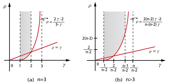
Remark 2.3.
For , if , then the inequality always holds true under the assumption (see Figure 1).
Definition 2.1.
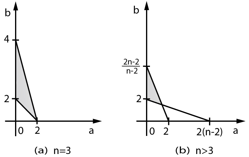
Remark 2.4.
One easily check that when . Moreover, if , then we can replace by , since (see Figure 2).
The energy associated to the problem (1.1) when is given by
We now state our main results.
Theorem 2.1.
Suppose that hold and let . Then given the initial data , there exist and a weak solution of problem (1.1). Moreover, the following energy identity holds for all :
| (2.13) |
Furthermore, if one of the assumptions hold: or
| (2.14) |
with , where
Then the solution of (1.1) is global.
Theorem 2.2.
Suppose that the hypotheses in Theorem 2.1 and (2.14) with and hold. Then we have following energy decay rates:
-
(i)
Case 1 : is linear. Then we have
where is a positive constant.
-
(ii)
Case 2 : has polynomial growth near zero, that is, . Then we have
-
(iii)
Case 3 : does not necessarily have polynomial growth near zero. Then we have
where and () are positive constants that depends only on .
Theorem 2.3.
Suppose that hypotheses with and hold. Moreover, assume that
and
| (2.15) |
where
Then the weak solution of the problem (1.1) blows up in finite time.
3. Proof of Theorem 2.1 : local existence
This section is devoted to prove the local existence in Theorem 2.1. The proof is based on three steps according to the following condition of the source term :
-
(1)
Existence of the global solution when is globally Lipschitz from to .
-
(2)
Existence of the local solution when is locally Lipschitz from to .
-
(3)
Existence of the local solution when is locally Lipschitz from to .
Then since the mapping is locally Lipschitz from to (see Remark 2.2), the existence of the local solution can be guaranteed even if .
3.1. Globally Lipschitz source
We first deal with the case where the source is globally Lipschitz from to . In this case, we have the following result.
Proposition 3.1.
Assume that hold. In addition, assume that and is globally Lipschitz continuous. Then problem (1.1) has a unique global solutions for arbitrary .
Our goal in this subsection is to show the local existence result for problem (1.1). We construct an approximate solution by using the Faedo-Galerkin method. Let be a basis in and define . Let and be sequences of such that strongly in and strongly in . We search for a function, for each and ,
satisfying the approximate perturbed equation
| (3.1) |
Since (3.1) is a normal system of ordinary differential equations, there exist , solutions to problem (3.1). A solution to problem (1.1) on some internal , will be obtain as the limit of as and . Next, we show that and the local solution is uniformly bounded independent of , and . For this purpose, let us replace by in (3.1) we obtain
| (3.2) | ||||
We will now estimate , and . From the hypotheses on , we have
| (3.3) | ||||
From the assumption , we have the imbedding , so that by Young’s inequality with we deduce that
| (3.4) | ||||
Under the assumption that is globally Lipschitz from into we have
where is the Lipschitz constant and is for some positive constant, so that by Hölder’s and Young’s inequalities and from the fact (2.1) and the imbedding , we deduce that
| (3.5) | ||||
where is an imbedding constant.
Replacing (3.3), (3.4) and (3.5) in (3.2) we get
| (3.6) | ||||
By integrating (3.6) over with we have
| (3.7) | ||||
Therefore, choosing and and then by Gronwall’s lemma we obtain
| (3.8) |
where is a positive constant which is independent of , and . The estimate (3.8) implies that
| (3.9) |
and
| (3.10) |
We note that from (3.8), taking the hypotheses on into account we also obtain
| (3.11) |
where is a positive constant independent of , and .
From (3.8)-(3.11), there exists a subsequence of , which we still denote by , such that
Since is compact, we have, thanks to Aubin-Lions Theorem that
and consequently, by making use of Lions lemma, we deduce
The above convergences permit us to pass to the limit in the (3.1). Since is a basis of and is dense in , after passing to the limit we obtain
| (3.12) | ||||
for all and .
Since estimates (3.8) and (3.11) are also independent of , we can pass to the limit when in obtaining a function by the same argument used to obtain from , such that
| (3.13) |
| (3.14) |
| (3.15) |
| (3.16) |
| (3.17) |
| (3.18) |
By above convergences in (3.12), we have
| (3.19) | ||||
Our goal is to show that . Indeed, considering in (3.1) and then integrating over , we have
Then from convergences (3.13)-(3.18) we obtain
| (3.21) |
By combining (3.20) and (3.21), we have
which implies that
| (3.22) |
Next, considering in (3.1) and then integrating over , we have
From (3.14)-(3.18) and (3.22), we arrive at
| (3.23) |
On the other hand, since is a nondecreasing monotone function, we get
for all . Thus, it implies that
By considering (3.15), (3.17) and (3.23), we obtain
| (3.24) |
which implies that .
We now show the uniqueness of the solution. Let and be two solutions of problem (1.1). Then verifies
for all . By replacing in above identity and observing that is monotonously nondecreasing and is globally Lipschitz, it holds that
Where is for some positive constant. By integrating from to and using Gronwall’s Lemma, we conclude that .
3.2. Locally Lipschitz source
In this subsection, we loosen the globally Lipschitz condition on the source by allowing to be locally Lipschitz continuous. More precisely, we have the following result.
Proposition 3.2.
Assume that hold. In addition, assume that and is locally Lipschitz continuous satisfying , where , are for some positive constants. Then problem (1.1) has a unique local solution for some .
Proof.
Define
where is a positive constant. With this truncated , we consider the following problem:
| (3.25) |
Since is globally Lipschitz continuous for each (see [10]), then by Proposition 3.1, the truncated problem (3.25) has a unique global solution for any . Moreover by [30] there exists a sequence of functions , which converges to in the class . For simplifying the notation in the rest of the proof, we shall express as .
By the regularity of , we can multiply by and integrate on , where . Then we obtain by using the fact for all ,
| (3.26) | ||||
We note that is globally Lipschitz with Lipschitz constant (see [10, 13]). Hence we estimate the last term on the right-hand side of (3.26) as follows:
| (3.27) | ||||
From the hypothesis on , we have
| (3.28) |
By replacing (3.27) and (3.28) in (3.26) and choosing , we get
| (3.29) |
for all , where
for . Thus by Gronwall’s inequality, (3.29) becomes
for all . If we choose
| (3.30) |
then
| (3.31) |
provided we choose . Consequently, (3.31) gives us that for all . Therefore, by the definition of , we have that on . By the uniqueness of solutions, the solution of the truncated problem (3.25) accords with the solution of the original, non-truncated problem (1.1) for , which means that the proof of Proposition 3.2 is completed.
∎
3.3. Completion of the proof for the local existence
In order to establish the existence of solutions, we need to extend the result in Proposition 3.2 where the source is locally Lipschitz from into . For the construction of the Lipschitz approximation for the source, we employ another truncated function introduced in [40]. Let be a cut off function such that
and for some constant independent from and define
| (3.32) |
Then the truncated function is satisfied the following lemma. The proof of this lemma is a routine series of estimates as in [1, 13], so we omit it here.
Lemma 3.1.
The following statements hold.
-
(1)
is globally Lipschitz continuous.
-
(2)
is locally Lipschitz continuous with Lipschitz constant independent of .
With the truncated source defined in (3.32), by Proposition 3.2 and Lemma 3.1, we have a unique local solution satisfying the following approximation of (1.1)
| (3.33) |
From Lemma 3.1, the life span of each solution , given in (3.30), is independent of since the local Lipschitz constant of the mapping is independent of . Also we known that depends on , where , however, since , we can choose sufficiently large so that is independent of . By (3.31),
| (3.34) |
for all . Therefore, there exists a function and a subsequence of , which we still denote by , such that
| (3.35) |
| (3.36) |
By (3.34), (3.35) and (3.36), we infer
| (3.37) |
for all . Moreover, by Aubin-Lions Theorem, we have
| (3.38) |
for . Since is a solution of (3.33), it holds that
| (3.39) |
for any , .
Now we will show that
| (3.40) |
Indeed, we have
| (3.41) |
By in Lemma 3.1 and (3.38), we obtain
| (3.42) | ||||
Since a.e. in , we have a.e. Then we also have and , for . Thus by the Lebesgue Dominated Convergence Theorem, we have
| (3.43) | ||||
Convergences (3.36), (3.37), (3.40) and (3.44) permit us to pass to the limit in (3.39) and conclude the following result.
Proposition 3.3.
Assume that hold. In addition, assume that and is locally Lipschitz continuous. Then problem (1.1) has a local solution for some .
Let , then is locally Lipschitz continuous (see Remark 2.2). Thus by Proposition 3.3, the proof of the local existence statement in Theorem 2.1 is completed.
3.4. Energy identity
It is well known that to prove the uniqueness of weak solutions, we will justify the energy identity (2.13). The energy identity can be derived formally by multiplying (1.1) by . But, such a calculation is not justified, since is not sufficiently regular to be the test function in as required in Definition 2.1. To overcome this problem, we employ the operator to smooth function in space, which is mentioned in Appendix A of [13]. We recall important properties of which play an essential role when establishing the energy identity.
Lemma 3.2.
([13]) Let . Then following statements hold.
-
(1)
If , then and in as .
-
(2)
If , then and in as .
-
(3)
If with , then and in as .
We will now justify the energy identity (2.13). We play the operator on every term of (1.1) and multiply by . Then we obtain by integrating in space and time
| (3.45) |
Since and , we have by Lemma 3.2, in and in . Therefore using this convergences, we have
| (3.46) |
Since , we easily check that
| (3.47) |
4. Proof of Theorem 2.1 : global existence
In this section we prove that a local weak solution on can be extended to . From the standard continuation argument of ODE theory, it suffices to show that is bounded independent of . We now consider the following two cases:
4.1.
Using the energy identity (2.13), we obtain
| (4.1) | ||||
By the same argument as (3.3), we have
| (4.2) |
Using the Hölder and Young inequalities with and the imbedding , we deduce that
| (4.3) | ||||
where is an imbedding constant. By replacing (4.2) and (4.3) in (4.1) and using the Young inequality and (2.8), we get
| (4.4) | ||||
Let
Choosing , we rewrite (4.4) as
where and are positive constants. Now applying Gronwall’s inequality, we have that , where and are positive constants. Consequently, since is bounded we conclude that is bounded.
4.2. The potential well
First of all, we will find a stable region. We set
and the functional
| (4.5) |
We also define the function, for ,
| (4.6) |
then
is the absolute maximum point of and
The energy associated to the problem (1.1) is given by
| (4.7) |
for . By (2.8) and (4.5)-(4.7), we deduce
| (4.8) |
Lemma 4.1.
Proof.
It is easy to verify that is increasing for , decreasing for , as . Then since , there exist , which verify
| (4.9) |
Considering that is nonincreasing, we have
| (4.10) |
From (4.8) and (4.9), we deduce that
| (4.11) |
Since , and is increasing in , from (4.11) it holds that
| (4.12) |
Next, we will prove that
| (4.13) |
We argue by contradiction. Suppose that (4.13) does not hold. Then there exists time which verifies
| (4.14) |
If , then we have, in view of (4.12), that there exists which verifies
| (4.15) |
Consequently, from the continuity of the function there exists verifying
| (4.16) |
Then from (4.8), (4.9), (4.15) and (4.16), we get
which also contradicts (4.10). This completes the proof of Lemma 4.1.
∎
By virtue of (4.17), we get
| (4.19) |
Hence
Therefore, there exists a positive constant independent of such that
| (4.20) |
Moreover, if we define the functional by
then from the relationship and the strict inequality (4.19), we obtain
| (4.21) |
Consequently, from (4.20) and (4.21) we have
This it the completion of the proof of the global existence of solutions of (1.1).
5. Proof of Theorem 2.2 : energy decay
In this section we prove the uniform decay rates for the solution of the following problem:
| (5.1) |
We consider the following additional hypothesis on :
| (5.2) |
Unless otherwise stated, the constant is a generic positive constant, different in various occurrences. We define the energy associated to problem (5.1):
Then
it follows that is a nonincreasing function.
First of all, we recall technical lemmas which will play an essential role when establishing the asymptotic behavior.
Lemma 5.1.
([35]) Let be a nonincreasing function and a strictly increasing function of class such that
Assume that there exists and such that
for all . Then has the following decay property:
Lemma 5.2.
([35]) Let be a nonincreasing function and a strictly increasing function of class such that
Assume that there exists , and such that
Then, there exists such that
Let us now multiply equation (5.1) by , where is given by
and is a concave nondecreasing function of class , such that as , and then integrate the obtained result over . Then we have
| (5.3) | ||||
We note that
and using Lemma 2.1 and the fact on ,
By replacing above identities in (5.3), we obtain
| (5.4) | ||||
Now we are going to estimate terms on the right hand side of (5.4).
;
Using the Young inequality and the inequality
we obtain
| (5.5) |
consequently,
| (5.6) |
;
From (5.5), we have
| (5.7) |
;
By the Young inequality with and from the fact is locally Lipschitz from into , (2.1) and (4.18) we get
| (5.8) | ||||
consequently,
| (5.9) |
;
From the Young inequality with , we have
Similar arguments as (5.8) we have
where . Hence we obtain
| (5.10) | ||||
By replacing (5.6), (5.7), (5.9) and (5.10) in (5.4) and choosing , small enough, we obtain from (5.2)
| (5.11) | ||||
Now we are going to estimate the last three terms on the right hand side of (5.11).
5.1. Case 1 : is linear.
Since is linear, we can rewrite the hypothesis of as follows:
for some positive constants , . Hence we get
| (5.12) |
| (5.13) |
| (5.14) |
| (5.15) |
| (5.16) |
and, since , it holds that . Consequently,
| (5.17) |
Let us set , where is for some positive constant, then satisfies all the required properties and we obtain that the energy decays exponentially to zero.
5.2. Case 2 : has polynomial growth near zero.
Assume that . Let , then we rewrite (5.11) as
| (5.19) | ||||
By hypotheses on and the Hölder inequality with , we have
and
Hence
| (5.20) | ||||
5.3. Case 3 : does not necessarily have polynomial growth near zero.
We will use the method of partitions of boundary modified the arguments in [35]. For every , we consider the following partitions of boundary depending :
if , or
if . Then (or ). Let us estimate , and on these partitions.
(I) Part on , .
(II) Part on .
(III) Part on , .
Using the fact is nonincreasing and is increasing, we have
| (5.29) | ||||
From (2.10), we obtain
| (5.30) | ||||
and
| (5.31) |
Therefore from (5.23)-(5.31), we deduce that
| (5.32) |
To estimate the last term of the right hand side of (5.32), we need the following additional assumption over (see [35], p.434):
Then by replacing (5.32) in (5.11) we obtain
| (5.33) | ||||
Define , . Then is strictly increasing and convex (cf. [35], [39]). We now take , then we can rewrite (5.33) as
which implies, by applying Lemma 5.2 with ,
Let be a number such that . Since is nondecreasing, we have
where , consequently, having in mind that , the last inequality yields
Then we conclude that
Therefore the proof of Theorem 2.2 is completed.
6. Proof of Theorem 2.3 : blow-up
This section is devoted to prove the blow-up result. First of all, we introduce a following lemma that is essential role for proving the blow-up.
Lemma 6.1.
Under the hypotheses given in Theorem 2.3 the weak solution to problem (1.1) verifies
Proof.
We recall the function, for ,
where . Then
is the absolute maximum point of and
The energy associated to problem (1.1) is given by
We observe that from the definition of , we have
| (6.1) |
Note that is increasing for , decreasing for , as .
We will now consider the initial energy divided into two cases: and .
Case 1 : .
There exist such that
| (6.2) |
By considering that is nonincreasing, we have
| (6.3) |
From (6.1) and (6.2) we deduce
| (6.4) |
Since , and is decreasing for , from (6.4) we get
| (6.5) |
Now we will prove that
| (6.6) |
by using the contradiction method. Suppose that (6.6) does not hold. Then there exists which verifies
| (6.7) |
If , we have, in view of (6.5), that there exists which verifies
| (6.8) |
Consequently, from the continuity of the function there exists verifying . Then from the last identity and taking (6.1), (6.2) and (6.8) into account we deduce
which also contradicts (6.3).
Case 2 : .
There is such that
consequently, by (6.1) we have
From the fact is decreasing for , we get
By the same argument as Case 1, we obtain
Thus the proof of Lemma 6.1 is completed.
∎
Now we will prove the blow-up result. In order to prove that is necessarily finite, we argue by contradiction. Assume that the weak solution can be extended to the whole interval .
Let be a real number such that
By setting , we have
| (6.9) |
which implies that is nondecreasing, consequently,
| (6.10) |
and from Lemma 6.1, (2.8) and the definition of ,
| (6.11) | ||||
We define
| (6.12) |
where and are small positive constants to be chosen later. Then we have
| (6.13) |
We are now going to analyze the last term on the right-hand side of (6.13).
Lemma 6.2.
| (6.14) | ||||
where is for some positive constant, , with and .
Proof.
We will now estimate the last term on the right-hand side of (6.15). We note that
By using (2.10) and the imbedding , we have
| (6.16) | ||||
On the other hand, by using (2.11), we obtain
| (6.17) | ||||
where and , are for some positive constants. Moreover implies that . Hence we get
From (6.10) and (6.11) we have
and, consequently, from (2.11), (6.9), (6.11) and (6.17),
| (6.18) | ||||
for . From (6.16) and (6.18), we get that
| (6.19) |
where .
By replacing (6.19) in (6.15) and choosing small enough we obtain
where is a positive constant. Therefore (6.14) follows.
∎
The following Lemma estimates the last three terms on the right-hand side of (6.14).
Lemma 6.3.
| (6.20) |
where and .
Proof.
From Lemma 5.1 and the definition of , we have
| (6.21) |
We note that
and
Since (2.15) holds, we get
Therefore, represents a curve connecting horizontal axis points and , and
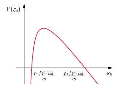
Thus we obtain
∎
Combining (6.13), (6.14), (6.20) and then choosing and small enough, we obtain
where is a positive constant, which implies that is a positive increasing function. By same arguments as p.333 in [16], we have
where is a positive constant and . Hence we conclude that blows up in finite time and also blows up in finite time. Thus this is a contradiction, consequently, the proof of Theorem 2.3 is completed.
Acknowledgments
This research was supported by Basic Science Research Program through the National Research Foundation of Korea(NRF) funded by the Ministry of Education (2022R1I1A3055309).
References
- [1] L. Bociu, Local and global wellposedness of weak solutions for the wave equation with nonlinear boundary and interior sources of supercritical exponents and damping, Nonlinear Anal., 71 (2009) e560–e575.
- [2] L. Bociu, I. Lasiecka, Uniqueness of weak solutions for the semilinear wave equations with supercritical boundary/interior sources and damping, Discrete Contin. Dyn. Syst., 22 (2008) 835–860.
- [3] L. Bociu, M. Rammaha, D. Toundykov, On a wave equation with supercritical interior and boundary sources and damping terms, Math. Nachr., 284 (16) (2011) 2032–2064.
- [4] Y. Boukhatem, B. Benabderramane, Existence and decay of solutions for a viscoelastic wave equation with acoustic boundary conditions, Nonlinear Anal., 97 (2014) 191–209.
- [5] S. Brenner and L. R. Scott, The Mathematical Theory of Finite Element Methods, Springer Verlag, 1994.
- [6] X. Cao and P. Yao General decay rate estimates for viscoelastic wave equation with variable coefficients, J. Syst. Sci. Complex, 27 (2014) 836–852.
- [7] M. M. Cavalcanti, V. N. Domingos Cavalcanti, I. Lasiecka, Well-posedness and optimal decay rates for the wave equation with nonlinear boundary damping-source interaction, J, Differential Equations, 236 (2007) 407–459.
- [8] M. M. Cavalcanti, V. N. Domingos Cavalcanti, P. Martinez, Existence and decay rate estimates for the wave equation with nonlinear boundary damping and source term, J. Differential Equations, 203 (2004) 119–158.
- [9] M. M. Cavalcanti, A. Khemmoudj, M. Medjden, Uniform stabilization of the damped Cauchy-Ventcel problem with variable coefficients and dynamic boundary conditions, J. Math. Anal. Appl. 328 (2007) 900–930.
- [10] I. Chueshov, M. Eller and I. Lasiecka, On the attractor for a semilinear wave equation with critical exponent and nonlinear boundary dissipation, Comm. Partial Differential Equations, 27 (9-10) (2002) 1901–1951.
- [11] Y. Guo and M. A. Rammaha, Global existence and decay of energy to systems of wave equations with damping and supercritical sources, Z. Angew. Math. Phys., 64 (3) (2013) 621–658.
- [12] Y. Guo, M. A. Rammaha and S. Sakuntasathien Blow-up of a hyperbolic equation of viscoelasticity with supercritical nonlinearities, J. Differential Equations, 262 (2017) 1956–1979.
- [13] Y. Guo, M. A. Rammaha, S. Sakuntasathien, E. S. Titi and D. Toudykov, Hadamard well-posedness for a hyperbolic equation of viscoelasticity with supercritical sources and damping, J. Differetinal Equations, 257 (2014) 3778–3812.
- [14] T. G. Ha, Asymptotic stability of the semilinear wave equation with boundary damping and source term, C. R. Math. Acad. Sci. Paris Ser. I, 352 (2014) 213–218.
- [15] T. G. Ha, Asymptotic stability of the viscoelastic equation with variable coefficients and the Balakrishnan-Taylor damping, Taiwanese J. Math., 22 (4) (2018) 931–948.
- [16] T. G. Ha, Blow-up for semilinear wave equation with boudnary damping and source terms, J. Math. Anal. Appl., 390 (2012) 328-334.
- [17] T. G. Ha, Blow-up for wave equation with weak boundary damping and source terms, Appl. Math. Lett., 49 (2015) 166-172.
- [18] T. G. Ha, Energy decay for the wave equation of variable coefficients with acoustic boundary conditions in domains with nonlocally reacting boundary, Appl. Math. Lett., 76 (2018) 201–207.
- [19] T. G. Ha, Energy decay rate for the wave equation with variable coefficients and boundary source term, Appl. Anal., 100 (11) (2021) 2301–2314.
- [20] T. G. Ha, General decay estimates for the wave equation with acoustic boundary conditions in domains with nonlocally reacting boundary, Appl. Math. Lett., 60 (2016) 43–49.
- [21] T. G. Ha, General decay rate estimates for viscoelastic wave equation with Balakrishnan-Taylor damping, Z. Angew. Math. Phys., 67 (2) (2016) Art. 32, 17 pp.
- [22] T. G. Ha, Global existence and general decay estimates for the viscoelastic equation with acoustic boundary conditions, Discrete Contin. Dyn. Syst., 36 (2016) 6899–6919.
- [23] T. G. Ha, Global solutions and blow-up for the wave equation with variable coefficients: I. interior supercritical source, Appl. Math. Optim. 84 (suppl. 1) (2021) 767–803.
- [24] T. G. Ha, On the viscoelastic equation with Balakrishnan-Taylor damping and acoustic boundary conditions, Evol. Equ. Control Theory, 7 (2) (2018) 281–291.
- [25] T. G. Ha, On viscoelastic wave equation with nonlinear boundary damping and source term, Commun. Pur. Appl. Anal., 9 (6) (2010) 1543–1576.
- [26] T. G. Ha, Stabilization for the wave equation with variable coefficients and Balakrishnan-Taylor damping, Taiwanese J. Math., 21 (2017) 807–817.
- [27] T. G. Ha, D. Kim and I. H. Jung, Global existence and uniform decay rates for the semi-linear wave equation with damping and source terms, Comput. Math. Appl., 67 (2014) 692–707.
- [28] V. Komornik and E. Zuazua, A direct method for boundary stabilization of the wave equation, J. Math. Pures Appl., 69 (1990) 33–54.
- [29] I. Lasiecka, Mathematical Control Theory of Coupled PDE’s, CBMS-SIAM Lecture Notes, SIAM, Philadelphia, 2002.
- [30] I. Lasiecka and D. Tataru, Uniform boundary stabilization of semilinear wave equations with nonlinear boundary damping, Differential and Integral Equations, 6 (3) (1993) 507–533.
- [31] I. Lasiecka, D. Toundykov, Energy decay rates for the semilinear wave equation with nonlinear localized damping and source terms, Nonlinear Anal., 64 (2006) 1757–1797.
- [32] I. Lasiecka, R. Triggiani, P. F. Yao, Inverse/observability estimates for second-order hyperbolic equations with variable coefficients, J. Math. Anal. Appl., 235 (1999) 13–57.
- [33] J. Li, S. Chai, Energy decay for a nonlinear wave equation of variable coefficients with acoustic boundary conditions and a time-varying delay in the boundary feedback, Nonlinear Anal., 112 (2015) 105–117.
- [34] L. Lu, S. Li, Higher order energy decay for damped wave equations with variable coefficients, J. Math. Anal. Appl., 418 (2014) 64–78.
- [35] P. Martinez, A new method to obtain decay rate estimates for dissipative systems, ESAIM: Control, Optimisation Calc. Var., 4 (1999) 419–444.
- [36] J. Y. Park, T. G. Ha, Energy decay for nondissipative distributed systems with boundary damping and source term, Nonlinear Anal., 70 (2009) 2416–2434.
- [37] J. Y. Park and T. G. Ha, Existence and asymptotic stability for the semilinear wave equation with boundary damping and source term, J. Math. Phys., 49 (2008) 053511.
- [38] J. Y. Park, T. G. Ha, Well-posedness and uniform decay rates for the Klein-Gordon equation with damping term and acoustic boundary conditions, J. Math. Phys., 50 (2009) 013506.
- [39] J. Y. Park, T. G. Ha, Y. H. Kang, Energy decay rates for solutions of the wave equation with boundary damping and source term, Z. Angew. Math. Phys., 61 (2010) 235–265.
- [40] P. Radu, Weak solutions to the Cauchy problem of a semilinear wave equation with damping and source terms, Adv. Differential Equations, 10 (11) (2005) 1261–1300.
- [41] I. E. Segal, Non-linear semigroups, Ann. Math., 78 (1963) 339–364.
- [42] E. Vitillaro, On the wave equation with hyperbolic dynamical boundary conditions, interior and boundary damping and supercritical sources, J. Differential Equations, 265 (2018) 4873–4941.
- [43] E. Vitillaro, On the wave equation with hyperbolic dynamical boundary conditions, interior and boundary damping and source, Arch. Ration. Mech. Anal., 223 (2017) (3) 1183–1237.
- [44] J. Wu, Uniform energy decay of a variable coefficient wave equation with nonlinear acoustic boundary conditions, J. Math. Anal. Appl., 399 (2013) 369–377.
- [45] P. Yao, Energy decay for the Cauchy problem of the linear wave equation of variable coefficients with dissipation, Chin. Ann. Math. Ser. B, 31 (1) (2010) 59–70.
- [46] P. F. Yao, On the observability inequality for exact controllablility of wave equations with variable coefficients, SIAM J. Control Optim., 37 (1999) 1568–1599.