Global Modeling of Nebulae With Particle Growth, Drift, and Evaporation Fronts.
III. Redistribution of Refractories and Volatiles
Abstract
Formation of the first planetesimals remains an unsolved problem. Growth by sticking must initiate the process, but multiple studies have revealed a series of barriers that can slow or stall growth, most of them due to nebula turbulence. In a companion paper, we study the influence of these barriers on models of fractal aggregate and solid, compact particle growth in a viscously evolving solar-like nebula for a range of turbulent intensities . Here, we examine how disk composition in these same models changes with time. We find that advection and diffusion of small grains and vapor, and radial inward drift for larger compact particles and fractal aggregates, naturally lead to diverse outcomes for planetesimal composition. Larger particles can undergo substantial inward radial migration due to gas drag before being collisionally fragmented or partially evaporating at various temperatures. This leads to enhancement of the associated volatile in both vapor inside, and solids outside, their respective evaporation fronts, or “snowlines”. In cases of lower , we see narrow belts of volatile or supervolatile material develop in the outer nebula, which could be connected to the bands of “pebbles” seen by ALMA. Volatile bands, which migrate inwards as the disk cools, can persist over long timescales as their gas phase continues to advect or diffuse outward across its evaporation front. These belts could be sites where supervolatile-rich planetesimals form, such as the rare CO-rich and water-poor comets; giant planets formed just outside the H2O snowline may be enhanced in water.
1 Introduction
Global models of the evolution of solids in the protoplanetary nebula are critical for understanding the sizes and composition of primitive inner and outer solar system bodies, their accretion timescale, and the meteorite record. Parent bodies of chondrites accreted over a few Myr, a time span over which models and observations of “dusty-gas” protoplanetary disks indicate that they evolved significantly (e.g., Villeneuve et al., 2009; Williams, 2012; D’Antona & Mazzitelli, 1994). Indeed, growing indications are that the very first planetesimals even form in the first Myr or less (Kruijer et al., 2017; Nanne et al., 2019). Understanding how these first bodies formed remains the most intractable question in addressing planet formation, because it is known that even weakly turbulent environments frustrate particle growth with a gauntlet of barriers. These barriers include bouncing and fragmentation (Güttler et al., 2010; Zsom et al., 2010), which slow or stall growth at pebble sizes, and radially inward migration due to aerodynamic drag (Weidenschilling, 1977; Cuzzi & Weidenschilling, 2006; Brauer et al., 2008; Johansen et al., 2014) which can remove particles faster than they can grow. Inward drift can transport material from the outer to inner disk and ultimately into the central star (Estrada et al., 2016, 2022, hereafter Papers I and II, and other studies noted below). Moreover, turbulence can even create “erosion barriers” that prevent incremental growth through the km size range (Ida et al., 2008; Morbidelli et al., 2009; Nelson & Gressel, 2010; Gressel et al., 2011).
These barriers have motivated an emphasis on essentially globally nonturbulent disks which allow dramatic vertical settling of particles and permit a variety of dense midplane particle layer instabilities (e.g., Goldreich & Ward, 1973; Goodman & Pindor, 2000; Garaud & Lin, 2004), with the currently most popular being the Streaming Instability (SI, Youdin & Goodman, 2005; Johansen et al., 2007; Carrera et al., 2017; Yang et al., 2017) that further concentrates the dense layer of settled particles such that eventual gravitational collapse can “leap-frog” clumps of relatively small particles directly into 100km-size planetesimals.
However, it is increasingly thought that protoplanetary disks in the early stages of their evolution when the first planetesimals and planets form are at least weakly-to-moderately-turbulent in the regions of the disk ( AU) in which particle growth is of the greatest interest (see e.g., Turner et al., 2014; Lyra & Umurhan, 2019, for reviews). Under such conditions, formation of planetesimals by SI is challenged or even precluded under self-consistent particle size assumptions (Umurhan et al., 2020, Paper II), at least for disks with cosmic (solar) metallicity. Meanwhile, a different “leap-frog” mechanism (Turbulent Concentration or TC) does operate in turbulence, and seems capable of producing large planetesimals directly from swarms of growth-frustrated “pebbles” under these conditions (Cuzzi et al., 2010; Chambers, 2010; Hartlep & Cuzzi, 2020).
The relative efficacy of these alternate mechanisms is strongly dependent on the gas turbulent intensity, the particle size and density, and the local metallicity, making high-fidelity, self-consistent models of early particle growth and transport in moderate turbulence critical. Previous global disk models (many of them assuming turbulence at various intensities) have focused on the dynamical evolution of the particle size distribution, and on determining the conditions under which planetesimals can form (Brauer et al., 2008; Birnstiel et al., 2010; Drażkowska et al., 2013, Paper I). In these models, relatively little attention has been given to the evolution of the composition of the planetesimals. There have also been a number of model studies aimed more specifically at the compositional variations one might expect, some including particle drift and diffusion, and mainly emphasizing the volatiles of the outer solar system (Öberg et al., 2011; Ali-Dib et al., 2014; Piso et al., 2015, 2016; Thiabaud et al., 2015; Öberg & Bergin, 2016; Booth et al., 2017; Cridland et al., 2017; Bosman et al., 2018; Krijt et al., 2018, 2020). These results resonate with a growing number of observational studies using ALMA and other facilities (Qi et al., 2013b, a; Cleeves, 2016; Zhang et al., 2020a, b; van der Marel et al., 2021, and others). However, the particle growth physics, radiative transfer, and global mass redistribution in most of these latter models has been significantly simplified to focus on the chemistry.
The composition of primitive bodies (the mineralogy and isotopic composition of primitive meteorite parent bodies, and increasingly detailed spectroscopy and in-situ sampling of comets) is rich in constraints on the environments in which they accreted. The rapid inward migration of solids can lead to significant redistribution of the nebula condensibles relative to the evolving gas over time, and alter the local chemical and isotopic composition. Variable C/O ratios affect the local oxidation state, and thus the mineralogy. Remote and in-situ observations of comets suggest that, while a substantial amount of mixing occurred over the solar nebula lifetime (Zolensky et al., 2006; Zanda et al., 2018) - most easily explained by nebula turbulence - there is also considerable compositional diversity in the comet and TNO populations (Barucci et al., 2008; Mumma & Charnley, 2011; Biver et al., 2018; Wierzchos & Womack, 2018; McKay et al., 2019). The complex meteorite record (e.g., Paper I, Kruijer et al. 2017; Nanne et al. 2019; Pignatale et al. 2019; Jacquet et al. 2019; Li et al. 2020b, 2021; Sengupta et al. 2022) strongly suggests that even the first few hundred thousand years of nebula evolution (the period covered by this paper) could have left us visible chemical and isotopic fingerprints.
In Paper I we developed our basic techniques and presented global evolutionary models of particle growth (as compact spheres) and drift, with self-consistent radiative transfer and local thermal structure. In our companion Paper II we present detailed global disk evolution simulations of porous (fractal) particle aggregate growth by adapting a previously developed particle aggregation and compaction recipe (Suyama et al., 2012; Okuzumi et al., 2012; Kataoka et al., 2013) to the basic code of Paper I. Paper II focused specifically on the evolution of the particle mass and internal density distribution, whereas here (Paper III) we focus on the radial variation of disk composition, and its evolution with time. We do not include a chemical model in our code. Rather, our disk model tracks a realistic mixture of refractory oxides (CAIs), silicates, iron metal and iron sulfide, refractory organics, and ices from H2O to the supervolatiles CO2, CH4, and CO, each with its own associated evaporation front (EF). As in both Paper I and Paper II, we include a self-consistent calculation of disk opacity and temperature which depends on the evolving size distribution in a fully evolving nebula. Our model is novel in its treatment of all this complexity simultaneously. In Section 2 we briefly summarize the most relevant physics for this paper, and refer the reader to Paper II for more detailed discussion. In Section 3 we describe the results of our simulations in the context of composition, comparing models with fractal aggregation and compaction to compact particle growth models. In Section 4 we present a discussion of some implications of our results, and in Section 5 we summarize our findings.
2 Nebula model
The simulations presented here and in Paper II are done using our parallelized D radial nebula code in which we simultaneously treat particle growth and radial migration of solids, while evolving the dynamical and thermal evolution of the protoplanetary gas disk. Our code includes the self-consistent growth and radial drift of particles of all sizes, accounts for size-dependent vertical settling and diffusion of the particles, radial diffusion and advection of solid and vapor phases of multiple species of refractories and volatiles, and a self-consistent calculation of the opacity and disk temperature that allows for us to track the evaporation and condensation of all species as they are transported throughout the disk. Our base code is described in detail in Paper I, while the model for fractal growth and its implementation is described in Paper II along with other changes and improvements to our code. Here we only summarize those elements that are germane to the compositional evolution of condensables.
2.1 Gas Disk Evolution
In our simulations we use initial conditions derived from the analytical expressions of Lynden-Bell & Pringle (1974), as generalized by Hartmann et al. (1998) and parameterized in terms of an initial disk mass and radial scale factor (Paper I). The resulting gas surface density distribution is fairly similar to that used by Desch (2007) and represents a denser inner nebula than the Minimum Mass Solar Nebula (MMSN, Hayashi, 1981). The time-dependent evolution of the gas surface density and gas radial velocity in one dimension are given by (Pringle, 1981)
| (1) |
| (2) |
where is the total viscosity parameterized in terms of a turbulent intensity . The viscosity depends on the evolving disk temperature both through the gas sound speed , and the nebula gas pressure scale height where is the local orbital frequency. The gas mass accretion rate is given by where indicates accretion towards the star, and indicates mass flux outwards. The radius at which flux reversal occurs depends on ambient nebula conditions and varies with time, tending to move outwards as the disk evolves. Its initial value can be given in terms of the radial scale factor at and is for our initial conditions (Hartmann et al., 1998). We take as a free parameter which sets the initial surface density profile in terms of the initial disk mass (see Paper II, ).
2.2 Evolution of Solid and Vapor Phases for Different Compositional Species
Our model tracks multiple species in both vapor and solid phases. In Table 2.2, we list the species used in this work along with their corresponding 50% condensation temperatures , compact particle density and initial mass fractions in the solid state , the latter of which are determined with data from Table 2 of Lodders (2003). Our nominal species and abundances differ slightly, however, for better alignment with recent studies of comets (Mumma & Charnley, 2011). To get our values for , we started with the initial refractory organics fraction (CHON, ratio of 1:1:0.5:0.12) from Pollack et al. (1994) as a guide, and then for simplicity partitioned the remaining C in the ratio of 1:1:1 in determining the fractions of CO, CH4 and CO2. The silicate abundances are initialized by placing all the Mg in orthopyroxene (MgSiO3) and olivine (Mg2SiO4), while the initial refractory iron fraction is what remains after all of the S is placed in FeS. Some of the remaining O is used in determining the Ca-Al fraction which is a mixture of Al2O3, CaO and CaTiO3, while the rest is placed in water. By contrast, Lodders (2003) has no refractory organics, assumes no O-bearing supervolatiles (i.e., CO, CO2), allows water to capture almost all the O that is not consumed by silicates, and assumes the C is in methane ice or in methane hydrate that travels with the water ice. In Table 2.2, we also compare the mass fractions in our work to those used by other workers. Here is the metallicity; for this work .
| Species | (K) | (g cm-3) | () | (L03)a | (P94)d | (B18)f | |
|---|---|---|---|---|---|---|---|
| Ca-Al | 2000 | 4.0 | 0.017 | … | … | … | |
| Iron | 1810 | 7.8 | 0.048 | … | 0.009 | … | |
| Silicates | 1450 | 3.4 | 0.220 | (0.204)b | 0.244 | 0.329g | |
| FeS | 680 | 4.8 | 0.085 | (0.125)c | 0.055 | 0.074 | |
| Organics | 425 | 1.5 | 0.258 | … | 0.252e | 0.397 | |
| H2O | 160 | 0.9 | 0.253 | 0.384 | 0.397 | 0.200 | |
| CO2 | 47 | 1.56 | 0.060 | … | … | … | |
| CH4 | 31 | 0.43 | 0.022 | 0.222 | … | … | |
| CO | 20 | 1.6 | 0.038 | … | … | … |
-
a
Table 11, first column of Lodders (2003)
-
b
This value includes silicates and oxides.
-
c
Includes all metals (e.g., refractory Fe) in addition to FeS
-
d
Table 2, third column of Pollack et al. (1994)
-
e
Does not include “volatile organics” such as CH3OH and H2CO used in Pollack et al.
-
f
Table 1, third column of Birnstiel et al. (2018)
-
g
Astronomical (amorphous) silicates from Draine (2003)
As the disk evolves, the solids (dust and larger, migrator particles, see below) and vapor fractions, denoted by d, m and v respectively, of each species change with time as particles grow and are transported throughout the nebula. The local instantaneous mass fraction, or concentrations of each species relative to the gas, in each phase, are given as functions of time by
| (3) |
or the ratio of the surface density of each species and phase to the gas surface density. The mass fraction of all species in a given phase is just the sum over in Eq. (3), e.g. for the dust, . Similarly, the local varying mass fraction for all phases of a given species is the sum over all i, , whereas the instantaneous metallicity, which includes all species in the solid state locally, is .
Particle growth in our code incorporates the physics of fragmentation, bouncing, erosion, and mass transfer (see \al@Est16,Est21; \al@Est16,Est21, and references therein) with mass, composition, and impact velocity-dependent sticking coefficients. Our code employs the moments method for the “dust” distribution (Estrada & Cuzzi, 2008, 2009) which assumes a powerlaw dependence ranging in mass from a monomer up to the fragmentation mass, and treats particle growth explicitly beyond that. This allows us to greatly speed up calculations and focus on the more interesting evolution of larger aggregates. A migrator then is a particle that is more massive than the fragmentation mass, tends to be fairly decoupled from the gas phase (Paper I), and their distribution is tracked individually by mass rather than as only part of a powerlaw. Examples of the particle mass distributions of many of the simulations used in this paper can be found in the Appendix of Paper II. The minimum size in our particle size distributions is a monomer of radius m, which has a mass of g when using the compact particle density of g cm-3 derived from the combination of all species listed in Table 2.2.
In our simulations we use a threshold fragmentation specific energy cm2 s-2 for silicates and more volatile ices than water (CO2, CH4, and CO) which we will refer to as supervolatiles (Musiolik et al., 2016), and adopt cm2 s-2 for water ice, which has been thought to be “stickier” than silicates (e.g., Wada et al., 2009; Okuzumi et al., 2012). By stickier, it is meant that much higher impact speeds are needed for fragmentation. Recent work suggests it may only be sticky over a limited temperature range near the condensation temperature of water ice (Musiolik & Wurm, 2019), thus we include simulations in which we account for this by adopting the silicate value of outside this range which we refer to as a “cold H2O ice” model (see Paper II and Umurhan et al., 2020, for more discussion).
The evolution of solid and vapor phases is determined for each species by the advection-diffusion equation (Desch et al., 2017)
| (4) |
where is the net, inertial space velocity (advection + drift), is the diffusivity and represents sources and sinks for species which include growth, radial transport and destruction of migrating material. For the vapor phase, and , whereas for the particles and depend on a particle’s stopping time111The stopping time is the time needed for gas drag to dissipate a particle’s momentum of mass and radius relative to a gas with local volume density . , usually expressed as the Stokes number . for the particles has two contributions, one imposed by the radial motion of the gas , and the second the radial velocity of the particle with respect to the gas, which depends on the normalized pressure gradient or headwind parameter
| (5) |
where is the pressure, is the nebula gas mass volume density, is the gas sound speed, and the local Kepler velocity (see Sec. 3.1). Depending on size and density, and local gas conditions, particles can be subject to different drag regimes that determine (see Paper II, Sec. 2.2.1). In the end, and are determined at any radius through a mass density-weighted mean over all particle masses. In Equation 4 above, the sign of the radial drift velocity for solids depends on particle mass. Massive particles tend to drift radially inwards (), while less massive ones can be radially advected outwards with the gas (). This effect is accounted for in our code for particles smaller than the fragmentation mass by determining the particle mass (where ) that separates the population of particles moving inward from that moving outward, and then using these relative mass fractions as weighting factors in solving the advection-diffusion equation for each population. For masses larger than the fragmentation mass, we account for drift (and diffusion) for all mass bins individually (see \al@Est16,Est21; \al@Est16,Est21, ).
2.3 Disk Thermal Evolution
The evolving size distribution affects the local disk temperature through the local opacity, so a self-consistent calculation of the disk temperature is essential to capturing the disk’s dynamical evolution. The midplane temperature is determined iteratively from
| (6) |
which represents a combination of internal heating due to viscous dissipation and external illumination by the stellar luminosity . The optical depths and are the Rosseland and Planck means, applied in optically thick and thin regions respectively. We assume a flared disk geometry with a general radial variation given by Chiang & Goldreich (1997) (see, also Kenyon & Hartmann, 1987; Ruden & Pollack, 1991):
| (7) |
Our simulations employ a time variable stellar luminosity using a model for a 1 M⊙ star by D’Antona & Mazzitelli (1994, also ), where the initial luminosity is roughly at the beginning of a simulation, and drops to after 0.5 Myr. Such a high luminosity means that EFs for the supervolatile species listed in Table 2.2 are initially located considerably further away from the star than would be suggested by equilibrium temperatures calculated using a main sequence luminosity. In our models then, the water snowline begins at around AU, similar to the post buildup stage in models that include infall (e.g., Drażkowska & Dullemond, 2018; Homma & Nakamoto, 2018). We will consider other evolutionary track models in the future (e.g., see di Criscienzo et al., 2009; Tognelli et al., 2011).
Using a temporally constant as given in Eq. 7 while employing a variable luminosity is a simplification, because the varying luminosity may be primarily due to a variable stellar size. The protostellar flux on the disk surface is the product (Eq. 6) and the effective value of may increase along with going backwards in time due to the increase in stellar radius. The net effect would probably be an amplification of the temporal decrease of over time as the luminosity decreases. Since the assumed value for from Chiang & Goldreich (1997) assumes a stellar radius at the small end of our range, this might imply a slightly warmer disk at the earliest times than we currently find, leading to some temporal shift in the radial locations of the various EFs. However, since the values of and are themselves not that well known, and the disk temperature only depends on the product of them to the 1/4 power, even where it would provide the dominant heating (in the outer nebula), this variation is unlikely to be a major effect.
The optical depths in Eq. (6) are functions of the temperature-dependent opacity as . We define the Rosseland and Planck mean opacities from the basic wavelength-dependent opacity in the standard way as:
| (8) |
To determine the for both compact and porous aggregate particles, we utilize the opacity model of Cuzzi et al. (2014) which contains realistic material refractive indices for the species listed in Table 2.2 from Pollack et al. (1994) and is easily modified to handle porous aggregates, while for the supervolatiles we adopt available values from the literature (Warren, 1986; Schmitt et al., 1989; Hudgins et al., 1993; Martonchik & Orton, 1994). For the dominant particle sizes and mid-IR wavelengths, scattering can be neglected.
2.4 Mass Transport Across Evaporation Fronts
Evaporation fronts (EFs) are locations in the disk where species-dependent phase changes between solids and vapor can occur, and these play an important role in the redistribution of refractories and volatiles that is the focus of this paper. Inwardly migrating particles can sublimate222It is possible for, e.g., iron or silicates (e.g., Nagahara et al., 1994) to be stable as a liquid under nebula pressures somewhat higher than ours (our nebula pressures inside 1 AU are in the bar range), but we do not include this complication in this work. How this would affect the stickiness of these species may be an important wrinkle to explore in the future. at various EFs, enhancing the gas phase there, while subsequent outward diffusion of vapor back across the EF can recondense onto grains there - significantly enhancing both the amount and composition of the resident material (e.g., Paper I, Ros & Johansen 2013; Schoonenberg & Ormel 2017). These processes have implications for chemistry, minerology, and planetesimal formation. We allow for the “phase” change to occur linearly over a small temperature range ( K) so that EFs are not necessarily sharp boundaries. Allowing for this gradual radial transition prevents unrealistic drops in opacity and temperature just inside an EF, and effectively mimics buffering of midplane temperature changes as material is evaporated or condensed at different altitudes (see Paper I, for more discussion).
The specifics of how changes in the mass fractions are treated as they are transported across EFs either through radial drift, advection or diffusion are described in Appendix A.3 (and Secs. 2.4.5-2.4.6) of Paper I. In our code, when inwardly transported solid material encounters an EF, their associated volatile is removed from the solid phase and transferred to the gas phase. As a by-product of the change in , the composition and masses of the particles and aggregates change. When material drifts inwardly into a new radial bin the released, volatile-free dust fraction is assumed to adjust to the local dust distribution, while the distribution of newly volatile-free migrators is explicitly added to the local population.
When vapor of the associated volatile diffuses outward across its EF, we assume that it recondenses instantaneously, and is partitioned onto both dust and migrator populations in the appropriate area fractions. Changes in the mass distribution affect the local opacity and temperature so that additional modifications to the local can occur when the new is calculated. Since most of the outwardly diffused volatile material condenses on the tiny grains with the most surface area, which can then coagulate with existing aggregates, the recondensed volatile is assumed to be uniformly mixed back into the local particles333 Our particles are treated as if they are aggregates of chemically distinct monomers.. We plan to address the details of phase changes, as well as more realistic models for particle architecture (see Sec. 4.3) in future work.
| a Model | Type | (cm2 s-2) | |
|---|---|---|---|
| fa2g | fractal | ||
| b fa3g | fractal | ||
| fa3Qg | fractal | ||
| fa4g | fractal | ||
| fa5g | fractal | ||
| sa2g | compact | ||
| b sa3g | compact | ||
| sa3Qg | compact | ||
| sa4g | compact | ||
| sa5g | compact |
-
a
All models have an initial disk mass of M⊙, and AU.
-
b
These are the fiducial models from Paper II.
3 Results
We analyze a specific set of compact and fractal aggregate growth models for different turbulent intensity (Table 2.4), originally presented in Paper II, where all simulations have AU and M⊙ for a central star of mass M⊙ with variable luminosity (Sec. 2.3). In our analysis here, we focus on the compositional evolution. We emphasize again that our models do not incorporate a proper chemical model, and thus we only follow the composition and phase of our initial set of condensable species over time. When we refer to the ‘inner’ and ‘outer’ disk as we often do in this paper, we mean inside and outside the water snowline, respectively. Details of the evolution of the particle mass, size, and porosity distributions can be found in Paper II.
3.1 Evolution of Ambient Disk Properties
In Figure 1 (panels a-f) we show a snapshot for both fractal aggregate (solid curves) and compact particle (dashed curves) growth models of the most relevant subset of disk properties after 0.5 Myr of evolution for turbulent intensity values of (black curves), (orange curves, which are our fiducial models from Paper II) and (red curves). The cyan region in each plot denotes the radial range over which the water snowline is located across all models ( AU) at this evolution time. The top left panel (a) shows the gas surface density . All models have the same initial profile defined by (indicated by the light grey dotted curve) and are characterized by a steep dropoff outside of (Hartmann et al., 1998). These can be compared to the standard MMSN surface density profile (; the blue line) with a disk gas mass an order of magnitude smaller than our (Hayashi, 1981). Naturally, the low case shows the least evolution except in those regions where the variation in is driven by strong variations in (panel c) through the viscosity, and radial variations in tend to be smoothed out with higher values of . By 0.5 Myr, the gas surface density for is well below the standard MMSN value due to being lost inwards to the star, and to rapid spreading outwards beyond the radius where the mass flux changes sign (at , this is , but this location tends to move outwards with time).
More interesting variation is seen in the solids surface density , and between fractal aggregate and compact particle growth models (panel b). Generally, particle growth leads to inward radial drift, as particles or aggregates decouple more from the gas phase and incur headwind-drag forces. Inward drifting particles eventually encounter an EF which can lead to vapor enhancement inside, and (if the sublimated species diffuses or is advected back across the EF) solids enhancement outside of it. This effect (and contrast) is seen most easily for at the H2O snowline at AU. It is also seen for but diffusion is stronger so the contrast is less outside the water snowline, but also inside due to the outward diffusion from the organics EF ( AU, more below). With higher , contrasts are mostly blurred out across all EFs.
Interior to the snowline (the inner disk), the differences in between fractal and compact growth models for a given are surprisingly not very significant, in spite of the fact that the fractal aggregate masses are orders of magnitude larger than their compact counterparts (see Paper II, ). This suggests that their drift rates are similar despite the disparities in mass, and indeed the Stokes numbers (panel f, see below) are similar for and . The most variation is seen in the case which is due to the aforementioned organics EF which is much broader, and more pronounced than the snowline. This is actually still the case for ; it is less noticeable here in but can be seen clearly in (see next section). Stokes numbers for the highest turbulent intensity case are generally even smaller than for the other cases so these particles remain much more coupled to the nebula gas.
Outwards of the snowline where the fragmentation energy threshold is much larger, things begin to diverge because both fractal and compact growth can proceed to much larger masses (and in fact many orders of magnitude larger for fractal aggregates, see Paper II). This means these particles and aggregates are subject to much more rapid radial drift, owing to their larger Stokes numbers (panel f), leading to marked drops in , which is even more evident in the local metallicity (see Sec. 3.2). The drop in characterizes both compact and fractal growth models for ; however, the drop in extends only to AU in the fractal models, whereas the compact growth models continue to systematically lose material from the entire outer disk. Even though fractal aggregates grow more massive than compact particles, their mass-to-area ratios and Stokes numbers St can remain smaller, allowing the fractal models to retain much more mass in the region AU over longer periods. This occurs because the aggregates further out in the disk have not yet compacted enough to have Stokes numbers comparable to compact particles. This is also reflected in panel (f) where aggregate are larger inside 20 AU, but drop significantly below the for compact particles outside this distance. The cold H2O ice models (grey curves, panels b and f) show this behavior only over a narrower region that corresponds to a modest range in temperature ( K), outside of which drops to the value for silicates so decreases. As a result, remains significantly higher for the cold ice models than the fiducial models since the compact particles and aggregates have lower and thus much longer drift times. In fact, in these models some material is being advected outwards due to the stronger gas coupling. Gas coupling also explains what is seen in the models for which also show no corresponding drop in - because solid material is being even more strongly advected outwards in this case by the more strongly viscously evolving gas The stronger gas motions for dominate because the values for the highest turbulent intensity case are still small, even though larger than the cold ice, lower models because the nebula gas density is much lower. We refer the reader to Paper II for detailed discussion of the evolution of the particle mass distribution.
In panels (c)-(e) of Figure 1 we plot the midplane disk temperatures , headwind parameter , and the Rosseland mean opacity . The headwind parameter (Eq. 5, Sec. 2.2; see also Paper II) is primarily what drives the inward radial drift of particles () relative to the gas444Incidentally, at no point in these simulations does , so no appreciable pressure bumps develop that could trap particles.. Variations in these plots can largely be attributed to the evolution of the particle mass distribution and vice versa. In panel c, locations in the disk where the temperature flattens are just interior to EFs. The most refractory EFs have long ago evolved inwards off the grid, but the EFs for FeS, organics and water ice are still present. The CO2 snowline is also present at AU; it is not visible in the temperature, but is visible as a peak or a kink in the surface density profile seen in panel b. The temperature profile for a MMSN (, Hayashi 1981) is given by the blue line. Variations in the Rosseland mean opacity largely mirror those of the solids surface density profile. We do not show the Planck mean opacity , but these appear largely similar, except in the innermost disk and in the outer disk (mostly beyond AU) where the optical depth is low (see Fig. 5, Paper II, for a comparison of these opacities for the fiducial model). It is interesting to note that the model for begins with the highest initial temperature, while begins with the lowest (e.g., see Fig. 1, Paper I, ), but it is the model with that remains the hottest after 0.5 Myr. As discussed in Paper II, models with tend to be the “sweet spot” for the most optimal combination of particle growth and retention of solids in these disk models.
3.2 Evolution of Solids and Vapors


In this section we look at the evolution of the solid and vapor fractions of the individual species listed in Table 2.2 for all the simulations listed in Table 2.4. As a simplification in this work, we treat sublimation and condensation at EFs as completely reversible - which for our “organic” species in particular is not realistic (see Sec. 4). We will refine this treatment in a future paper. Our main goal herein is to study the radial and temporal variation of solid and vapor composition for the different models due to the effects of advection, diffusion and radial drift.
3.2.1 Fiducial Model
In Figure 2 we first examine the compositional evolution for a compact particle growth model with our fiducial turbulent intensity , also assuming a gaussian particle collision velocity pdf (case sa3g, see Paper II). Plotted in the top set of panels are the log of the solids mass fractions of the various species , at three different times, 0.1, 0.3 and 0.5 Myr. The bottom panels are the corresponding vapor fractions . Though locations of EFs can be seen in both sets of panels, they are the most easily seen in the vapor. In both sets of panels, the black dotted curves are the total fractions of solids or vapors, respectively, which for the solids also represents the locally varying metallicity (Sec. 2.2).
Mass Loss: The first thing to note is the systematic depletion of solid material outside the snowline, that occurs over time due to inward radial drift of material. As a result the inner disk regions become enhanced with solids while the outer disk becomes depleted. The depletion is especially rapid slightly beyond the water ice EF (cyan) because the mass-dominant particles here have the largest Stokes numbers () and thus the fastest radial drift (see Fig. 1 panel f, and Paper II, ). Recall that for the models shown, particles and aggregates can grow much larger everywhere beyond the water snowline due to the stickiness of water ice (Sec. 2.2). The particle sizes that correspond to these Stokes numbers are cm for the compact particle case, and m for the fractal case (see Appendix A, Paper II). As a result, the local drops by about an order of magnitude from the initial value in only years. In the inner disk, the solids enhancement appears to peak around 0.3 Myr with between AU, primarily due to enhancement of solids outside the organics EF (orange). However, because the Stokes numbers of the mass dominant particles are small in the inner disk, with , the local solids-to-gas volume density ratio so streaming instability is precluded even for this (see Paper II, ). In any case, the magnitude of this narrow peak in is probably an overestimate because sublimation-condensation of organics is likely not completely reversible as we assume here (see Sec. 4.3, and Paper II for more discussion). On the other hand, the sublimation and condensation of troilite (FeS, green) is likely reversible (Arm et al., 1960), but possibly only down to temperatures of K (see, e.g., Pasek et al., 2005). When sublimated, FeS transitions to H2S and refractory iron in the fraction 56/88 (see e.g., Paper I, ). This explains the sharp increase in refractory iron (red) around AU, inside the FeS EF. For this work we implicitly assume condensation back to FeS outside the troilite EF if refractory Fe is available there (however see Sec. 4.3).
Evaporation Fronts: In the outer disk, enhancements in supervolatiles CO (grey), CO2 (pink) and CH4 (yellow) can be seen outside their respective EFs, which evolve inwards as the disk cools (mostly due to decreasing stellar luminosity). A large enhancement spike in solid CO is seen at 700AU after 0.1 Myr, while all other solid species’ fractions have systematically decreased in magnitude. This enhancement is not due to inward radial drift of particles, because early on in this region of the disk where the gas density is so low, even monomers have very large Stokes numbers and are effectively immobile. Rather, this enhancement is due to the nebula gas advecting outward as the gas disk spreads. In our models, the initial gas surface density profile drops off sharply outside of AU (see Fig. 1, panel a) so that even small changes can make a significant difference in the local solid fractions in the outermost parts of the protoplanetary disk. Even though the nebula gas density remains very low, it has increased by orders of magnitude over the initial value, resulting in decreased instantaneous of all species except CO. The CO is enhanced because vapor phase CO is advecting with the nebula gas and condenses outside the CO EF at a rate fast enough to produce the relatively large spike in solid CO fraction. The magnitude of the spike eventually decreases over time once the advected nebula gas begins to increase significantly enough beyond the CO EF as the disk continues to spread outwards. The particle Stokes numbers in this outermost region then decrease, to unity or less, at which point the region can be vacated due to rapid radial drift (e.g., see top left panel of Fig. 6).
The methane and CO2 EFs lie inside AU and thus exhibit a different behavior because the particle Stokes numbers are . Both EFs have solids enhancements that extend outwards over many AU, with the CH4 enhancement being especially extended. This is because (like the case for CO) each region is enhanced already by the outward diffusion of sublimated vapor and subsequent recondensation outside their respective EF, as well as the outward advection of the nebula gas, but here the nebula gas can effectively advect small particles with it as well. The peak for CH4 is broader because the Stokes numbers of the mass-dominant particles are about an order of magnitude smaller than they are at the CO2 EF, and the gas advection velocity is increasing sharply in this region and is higher at the methane EF. Thus, small-St particles are advected further at the methane EF.


The bottom panels of Fig. 2 indicate that there are seven EFs still on the computational grid after 0.1 Myr (all 9 are present at ), so for the times shown, both iron and Ca-Al (“CAIs”, blue) are solid everywhere in the disk. The silicate EF (brown) persists for quite some time, but has evolved inwards off our inner grid boundary at 0.5AU by 0.5 Myr. Because the location where the nebula gas velocity switches from outwards to inwards occurs at AU, the enhancements in solids outside the various EFs in the inner disk tend to be due purely to diffusion for these models, while similar EF enhancements outside 20AU are due partly to advection. It is noteworthy that the enhancements in the metallicity of the gas can also become substantial (5-8%). This could systematically increase the local gas molecular weight, affecting the pressure gradient (and viscosity) through both the gas density and the local sound speed (see, e.g. Charnoz et al., 2021). A feedback effect from the increasing molecular weight of the gas might possibly lead to a pressure bump. This becomes more of an issue for lower . We will consider this effect more carefully in future work.
Fractal aggregate vs. compact particle growth: In Figure 3, we show a fractal aggregate growth model (fa3g) for the fiducial for comparison with the compact particle growth simulations of Figure 2. Many of the trends described for the compact growth case are also seen here. For example, the sharp decrease in total solids abundance outside the water ice EF ( AU) still occurs, with the solids surface density profiles overall being very similar (Figure 1). Like in model sa3g, the metallicity in the region from the H2O EF out to AU (dotted black lines in top panels of Fig. 2 and 3) has dropped to , because the St in this region are similar for sa3g and fa3g (; see Fig. 1, panel f)555It should be understood that growth to large and decreasing occur concomitantly. That is, the local is low because the local is large, and and are never both large enough at the same time and place that conditions for the Streaming Instability can be satisfied (see \al@Est16,Est21; \al@Est16,Est21, and also Umurhan et al. 2020).. The main difference is that now beyond AU much more material is retained because the fluffy aggregates have Stokes numbers times smaller than the compact particle case (orange curves, Fig. 1, panel f), though the fractal masses are several orders of magnitude larger than their compact counterparts (see Fig. 2, Paper II). Again, this is because aggregates have not yet compacted enough, so their St remain lower. The aggregates thus have much slower inward radial drifts, and a fraction of them can even be advected outwards. Indeed, where we saw much of the solids being depleted in the region AU in Fig. 2 leaving a clear enhancement in narrow supervolatile bands of CO2 and CH4 solids, the outer edge of this region remains populated with particles in the fractal case and has actually moved outwards from to AU over 0.5 Myr. The supervolatile bands are still present for the fractal case, but are very much muted (see Sec. 4.1). The differences can also be seen in the profiles (panel b, Fig. 1). Eventually though, we expect even the fractal aggregates outside AU will continue to compact and drift into the inner disk. The vapor fractions are similar in both models with the exception that the enhancements inside the supervolatile EFs are somewhat reduced.
“Cold (non-sticky) H2O ice”: In Figure 4 we show simulations for compact particle (sa3Qg) and fractal aggregate (fa3Qg) growth simulations for , which differ from the fiducial model in that we here assume that water ice is only “sticky” in a limited temperature range near the snowline (Musiolik & Wurm, 2019). We implement this in our simulations by only using the “sticky ice” (see Table 2.4) within 20 K of the water ice condensation temperature, and adopting the lower (silicate) value of at lower temperatures. In Fig. 4 we only show the solids fractions for the “cold ice” models at 0.5 Myr. One finds that for both fractal and compact particles, the depletion outside the snowline has been significantly reduced, because particles and aggregates cannot grow to nearly as large St further out in the disk, decreasing the mass influx of material. The region near the H2O EF in which and the fragmentation threshold remain high still has larger particles, with similar at their peak to the fiducial case (Fig. 1, panel f), but dropping off by nearly 2 orders of magnitude from there outwards. Enough material drifts in to prevent as large a drop in as seen in the fiducial model, but because less material drifts across the water ice EF overall, the enhancements in the inner disk are also smaller. The fractal case fa3Qg shows slightly more retention of material in the outermost portions of the disk than the corresponding compact particle case sa3Qg, but the latter retains much more than the fiducial compact particle growth case sa3g due to the smaller (Fig. 1).
3.2.2 Variation with Turbulence Parameter


Larger (): Simulations where we increase the turbulence parameter to are shown in Figure 5. Because relative velocities between compact or aggregate particles increase with , the fragmentation sizes and Stokes numbers are considerably smaller (at least initially) so that they remain more well coupled to the nebula gas and less affected by radial drift. As a result, the enhancements of solids and vapors at EFs are more muted overall compared to the fiducial models, and less material is lost from the outer disk. There is essentially no difference seen between compact and fractal growth in the evolution of the vapor species (2nd and 4th rows) over the course of the simulation.
New result on Fe and FeS: However, some interesting behavior is seen for the particles in the inner disk. In the compact growth model (1st row), the condensed FeS outside its EF appears to have the strongest enhancement - similar to or even larger than seen at the organics and water EFs. This FeS-enrichment comes at the expense of a dramatic depletion in iron metal near AU. This interesting effect, which actually begins around 0.2 Myr (not shown) in both fractal and compact growth models, occurs because the quick diffusion of a substantial amount of H2S across the FeS EF is reacting with inward drifting, native Fe metal to produce a large spike in condensed FeS, but the Fe metal is not replaced as quickly by inward radial drift of material from further out. By 0.5 Myr and beyond though, enough Fe dust is drifting in to begin to erase the Fe-depletion signature. This localized Fe-depletion is not seen in the fiducial model where the enhancement in FeS is absent, and instead the refractory iron is enhanced interior to the troilite EF. This Fe-depletion disappears sooner in the fractal aggregate growth model (mostly absent by 0.3 Myr) for this large (3rd row of Fig. 5) because, due to slower radial drift (smaller St in the inner disk overall), the enhancement of H2S, and its feedback across the EF, does not build up sufficiently to cause a depletion in refractory iron for nearly as long. We discuss this further in section 4.1.
Global evolution with time for vapor and solids: As pointed out above, there is no notable difference between the compact and fractal cases in the vapor evolution for the models, and at 0.1 Myr, the solids fractions in the outer disk regions beyond the snowline (1st and 3rd rows) also look quite similar. This changes gradually at later times. For both fractal and compact cases as the gas disk spreads outwards and the gas surface density increases significantly beyond AU (see panel a, Fig. 1), particles and aggregates are more easily advected outwards with the nebula gas, whose velocity increases strongly beyond AU. Outside AU, the of the fractal aggregates are smaller than their compact counterparts and are thus more coupled to the gas, so they are transported outward in greater abundance. This explains the slight difference in between the models at large distances at later times.
The rapid gas evolution for also decreases the gas density everywhere inside of AU significantly, and generally increases (red curves in Fig. 1, panel f) to values comparable to or even larger than the lower models despite being smaller in mass in comparison (cf. Figs. 2 and 8, Paper II, ). The differences in particle mass between the compact and fractal cases is still a few orders of magnitude (Fig. 8, Paper II, ), but the Stokes numbers of the mass dominant fractal aggregates are roughly the same for the compact and fractal growth cases, between the snowline and 90AU. We note that the much higher level of coupling between particles and the gas in both cases more or less maintains close to its initial value across the disk. This is largely true even in the inner disk, though there are slight enhancements in the solids outside EFs out to the snowline (including even the silicates at 0.1 Myr) in the compact particle growth simulation. Overall it appears the distinction between compact particle and fractal aggregate models diminishes for increasing .
Smaller : The change in overall behavior for smaller is much more dramatic, especially for compact particle growth, as can be seen for the case of plotted in Figure 6. The top panel (1st row), for the compact particle growth case, shows that the outer disk is much more quickly drained of solids to the inner disk regions compared to the fiducial model for compact particles, and also that material within the inner disk continues to be lost through the inner boundary and presumably to the star. The values of the mass dominant particles for both fractal and compact growth models are still relatively small and similar to each other (Fig. 1), but now an order of magnitude larger than in the fiducial model (so is the gas surface density). Similar St between sa4g and fa4g also means the loss rate of particles is roughly the same for the compact and fractal aggregate growth cases (1st and 3rd rows) inside the snowline despite the aggregates being 2 orders of magnitude larger in mass than the compact ones (see Fig. 8 Paper II, ). The exception is the extended knee inwards of the snowline from AU seen in Fig. 1 (panel f). We note that this region inside the snowline corresponds to a sharp drop in the normalized pressure gradient, or headwind parameter (panel d), which would slow the radial drift rate in the region inside the snowline. For the fractal aggregates, the temperature (panel c) is hotter and has a steeper gradient in this region (which corresponds to the organics EF). Coupled with the enhancement in organics, this drop in the headwind parameter allows aggregates that decreased in mass (due to loss of water) upon crossing the snowline to grow significantly larger again (compared to the compact particle case, see black curves Fig. 1, panel f) before drifting to the organics EF where considerable material is evaporated, so that aggregate Stokes numbers and particle masses plummet. The spike in water ice outside the snow line is also lower, meaning that aggregates that cross the snowline are less ice rich compared to the compact particle case, so they lose less mass as they cross this EF. The same effect is not seen in model sa4g because the dip in is further inward and not as large in magnitude.
Both fractal and compact particle growth cases see large enhancements in vapors inside, and in solids outside, the organics EF giving local (solids) as high as . The overall curves inside the snow line look very similar in magnitude for both models, but differences in their are notable (Fig. 1, panel b). The silicates EF also contributes to the local enhancement of , and persists longer in the fractal aggregate case. That is, the compact growth model cools much more quickly (see below). The enhancements in vapor (2nd and 4th rows) are considerably larger than in the fiducial model after 0.5 Myr, reaching values as high as and helping to produce the large enhancement in solid organics exterior to its EF. However, as noted previously, the solids fraction just outside the organics EF may not be realistic because the sublimated or decomposed CHON organics might break down into more volatile constituents such as CO or CH4, rather than recondense as a CHON. This would not greatly affect the enhancement to the total vapor fraction, which gets quite large in this region at least until these constituents have time to diffuse. As mentioned in Sec. 3.2.1, such large values for the vapor fraction further indicate that consideration of changes in the gas’ molecular weight may become important.


Fe-FeS behavior: The depletion of refractory iron over a small radial range is even more dramatic in this case than it was in the case for , and unlike the latter case, the depletion is not temporary. For both the compact and fractal growth cases (1st and 3rd rows), the depletion of refractory iron begins very early ( Myr) and the radial region over which this depletion grows increases with time as the excess diffusing H2S gas gobbles up available Fe, maximizing the amount of troilite that can be sublimated again at the EF. The feedback creates so much excess H2S that it diffuses further outward until it can react with more refractory iron further out in the disk. This process thus creates a situation in which troilite and H2S coexist out to as far as AU in the compact growth case, and somewhat less in the fractal case (2nd and 4th rows), though with time we would expect the situation to extend further out, as it did in the case with . Recall this effect is not seen in the fiducial model. Although it is not clear why the model does not show this effect, we suspect that it is because the inner disk remains hotter, longer than the lower and higher models (see Fig. 1, panel c). Despite the more rapidly drifting compact and aggregate particles (due to their higher St overall), Fe still cannot drift in fast enough to overcome this effect; presumably the effect could continue until most of the S from a range of radii is utilized (for more discussion see section 4.1).
Much like we saw in the fiducial case, the region outside the snowline is significantly depleted in solids, as growth there is rapid due to the higher threshold for ice. However, depletion in this region is especially rapid and substantial in the fractal aggregate growth model (3rd row). Even after 0.1 Myr the region between AU sees a large drop in the local metallicity that is absent in the compact particle case at this juncture. The more rapid growth of fractal aggregates comes about in large part due to their larger cross sections (Paper II). As aforementioned, particle Stokes numbers inside the snowline are similar between the compact and fractal models (with the exception of the knee region from AU), but outside the water ice EF fractal growth has led to mass-dominant aggregates with about a factor of 5 larger than the compact particles. In fact, by this time, the aggregate masses are already as much as 6 orders of magnitude more massive than the compact particles in the same region (see Fig. 9 of Paper II, ). This leads to initially more rapid drift of solids into the inner disk regions and explains why, at the early time of 0.1 Myr, there is more enhancement in the inner disk for the fractal case. But the rapid depletion means that by later times the net inward flux of material is lower than in the compact case which steadily drains into the inner disk. This is because in the fractal case, the mass-dominant aggregate drops below that of the compact case outside of AU by a factor (Fig. 1, panel f) so their drift rates are much slower, and considerable material remains there. On the other hand, rapid, continuous drift in model sa4g accounts for the much larger enhancement spike at the snowline in that model. By 0.5 Myr, the compact growth case has effectively lost most all of its material outside the snowline, while the fractal case retains a significant fraction.
Supervolatile bands? An effect of strong radial drift of disk material in the compact growth model case is the “trapping” of material that manifests as bands of supervolatiles centered at AU (CO2), AU (CH4) and beyond AU (CO). The magnitudes of these spikes in decrease over time, but for different reasons, as discussed for the fiducial model. We noted before that the region between AU is quickly vacated666This specific radial range is not special but will vary with the choice of . A larger (smaller) value of would move this location outwards (inwards). Indeed, a smaller may better correspond to an early stage disk subject to infall., even for small particles, because the Stokes numbers are already of order unity or larger there, so radial drift is rapid. On the other hand, outside AU, Stokes numbers become increasingly large due to the sharply decreasing gas density so the particles and aggregates are not drifting much at all. The decrease in mass fraction there is solely due to the slow expansion of the nebula gas disk over time, which in this low case is too slow to diminish the CO peak after 0.5 Myr compared to the fiducial model. Also as before, the band of CH4 is seen to be more extended in the fractal model due to the slower drift rates of the porous aggregates compared to the compact particles. It should be noted that these bands do not have a lot of mass, at least at this epoch, as can be gleaned from panel (b) of Fig. 1. For the compact growth model where a clear CO2 band is seen, there is a peak surface density of g cm-2, while for methane it is a hundred times smaller. The fractal model has a similar magnitude for CH4, but at the CO2 EF most species (Fig. 6, 3rd row and panel) are still present thanks to the low radial drift speeds of the porous, fluffy aggregates there (see also Fig. 8) so the fraction of CO2 is 2 orders of magnitude larger.


Temperature variations with : Amongst the above models, previously we mentioned that the fiducial model () remains the hottest after 0.5 Myr (Fig. 1, panel c), and at earlier times there is variation in the cooling rates of the disk amongst the different models. This is not difficult to understand. The case is cooler than the fiducial model despite having smaller particles and aggregates, which increases the opacity (Fig. 1, panel e), simply due to the order of magnitude decrease in gas density by 0.5 Myr compared to (Fig. 1, panel a). The compact particle growth case with is only marginally hotter than the corresponding high turbulence case because even though there is so much more nebula gas (and much more solids mass) for , the opacity has decreased significantly due to rapid particle growth. The fractal case for the low turbulence value stays hotter longer than the compact growth case for this , as seen in Fig. 6 (4th row) where the silicate EF persists up to 0.3 Myr, whereas it has already evolved inward of our computational inner boundary in the compact particle growth case by 0.1 Myr.
Extremely low case: Finally, in Figure 7 we present models for . The compact (sa5g) and fractal (fa5g) cases provide an even starker contrast to the models than did . For the compact particle growth case, such a low turbulent intensity leads to rapid loss of most solid material in a considerably shorter period of time than for . The end result is that after 0.3 Myr essentially only the banded EF-related structures remain, which only fade slightly after 0.5 Myr. The spike in H2O ice at its EF actually increases slightly, due to condensation from a large reservoir of vapor phase water as the disk cools and the EF moves inwards. The fractal aggregate case fa5g proceeds in a similar fashion to fa4g, with rapid growth outside the snowline to aggregate masses about an order of magnitude larger even than the model ( g, see Fig. 10, Paper II), and correspondingly larger . The larger quickly lowers the local to values . For this , advection and diffusion by the nebula gas are of course very small. It is clear that even for this low , the solid material in the fractal growth case persists longer than for the compact particle growth case, but unlike model fa4g, much of the mass in fa5g is gone by 0.5 Myr. However, we do find for this lowest that there is a short period of time at Myr where the solids-to-gas ratio just outside the snowline in both growth models is greater than unity and, with both the mass-dominant compact and aggregate particles having large , may briefly satisfy conditions for the streaming instability (see Umurhan et al., 2020) and a burst of ice-rich planetesimal formation. This is discussed in detail in Section 4.1 of Paper II.
4 Discussion
4.1 Bulk Planetesimal Composition
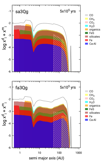
Following the evolution of refractories and volatiles as they are transported throughout the nebula allows us to say something about what the bulk composition of a planetesimal might be if it formed at a particular location in the protoplanetary disk, and at a given time. A general idea can be gleaned from the various evolutionary plots in Sec. 3.2, but here we generate a more direct visualization for specificity at 0.5 Myr, when silicates are condensed everywhere. We caution again that our simulations do not include a chemical model, but merely track our selected species as they evolve and change phase.
Figure 8 represents a snapshot of potential planetesimal composition for different values of . The left panel shows the compact growth models and the right panel the fractal aggregate growth models for turbulent intensities, from top to bottom, , and (Table 2.4). The locations of EFs, of which there are six still present in each simulation, are more easily seen in these figures as the radial location of the innermost boundary of a given species. The inner disk (region inside the snowline) is naturally the most refractory, but the variation in composition can be quite dramatic depending on and model type. In the outer nebula, temperatures are determined by stellar irradiation and not viscosity, so the locations of the EFs do not vary with ; the contents do, however. In the inner nebula, the fiducial case remains the hottest after this amount of time in the simulations (see Sec. 3.2.1), so even as far out as 1 AU, composition is dominated by silicates, iron and “CAIs”. In the colder models at other , or beyond 1 AU for , FeS contributes a significant fraction to the bulk composition. As we explained in Sec. 3.2.2, the models for actually have no refractory iron over a wide region from 0.4AU - 2AU, as it has all been incorporated in troilite leaving a large reservoir of H2S gas. It may be that this reservoir of H2S gas goes on to affect mineralogy in other ways that are beyond the scope of this paper (Lehner et al., 2013, 2017, see section 4.3). Alternately, some of the iron could be sequestered in silicates. For example, our models initially begin with Mg-rich orthopyroxene (enstatite) and olivine (forsterite) silicates only, but once silicates are evaporated and recondense, the emergence of Fe-rich silicates (e.g., fayalite and ferrosilite) might be possible. As mentioned earlier, we have not included chemistry or mineralogy in our model yet because it depends in a complicated way on the oxidation-reduction state of the local nebula, which can be influenced by the changing state or abundance of carbon as well as by variation in the silicate and/or H2O vapor abundance (Ebel & Grossman, 2000; Tenner et al., 2015, see also below and section 4.3). Further out still, “moderately refractory” organics (Pollack et al., 1994) which contain much of the C, can begin to dominate composition even creating a strong band of organics for the low turbulence case. This would suggest the possibility of very organic-rich bodies (a “tarline”, e.g., see Lodders, 2004), though as we have already mentioned, the enhancement of solid material outside the organics EF is likely overestimated in our current models because the organics probably break down into other constituents such as CO, NH3 and/or hydrocarbons (e.g., C2H2) which would not recondense locally or in their “moderately refractory” original form.
Just outside the H2O snowline ( AU in these models), there can be a large enhancement in water ice which can extend up to an AU or more outwards. If Jupiter’s core formed at the snowline, this effect suggests that it might have benefited from a spike of enhanced water relative to silicates (see also Kalyaan & Desch, 2019). However, the composition of the Jovian “core” is not clear, and results from Juno imply that the atmosphere is depleted in water relative to other heavy element abundances, and could even be sub-solar (Helled et al., 2022). Further outside the snowline out to about AU the composition is fairly uniform over the rest of the giant planet forming region (due to a lack of EFs there). Recall that this region is also expected to show a systematic depletion of solids due to inward radial drift. The lack of EFs suggests that the inwardly migrating particles may be able to drift relatively unaltered over much of this region, even as temperature increases. Jupiter is enhanced in C/H (as well as for noble gases and other volatiles) by a factor of (Mahaffy et al., 2000; Wong et al., 2008; Bolton et al., 2017; Li et al., 2020a). One suggestion has been to attribute this enhancement to supervolatiles being trapped in crystalline ice as clathrate-hydrates (e.g., Hersant et al., 2008; Mousis et al., 2009). An alternative is for supervolatiles to be trapped in amorphous ice in the colder regions of the disk (e.g., Bar-Nun et al., 2007, also see Monga & Desch 2015) that can be delivered to the giant planet region, but would have to be retained when amorphous ice transitions to crystalline (e.g., Ruaud et al., 2016). The presence of Ar, which clathrates only at very low temperatures ( K), as well as the presence of supervolatile ices on the giant planet moons, may favor the latter scenario (e.g., see Estrada et al., 2009, for more discussion).
Interestingly, in the very outermost portions of the disk, the supervolatile bands seen in models with suggests that it may be possible to have extremely supervolatile rich bodies that are essentially devoid of water forming in the coldest portions of the nebula, if planetesimals could form from the material “trapped” in these bands. Intriguing evidence along these lines may be found in the rare comets that are highly depleted in H2O relative to CO, such as Comets C/2016 R2/PanSTARRS, C/1908 R1 Morehouse, and C/1961 Humason (Biver et al., 2018; Cochran & McKay, 2018; McKay et al., 2019). In R2/PanSTARRS, CO/H2O was enhanced by a factor of 1000 over normal comets. These condensation bands will continue to evolve inwards as the disk cools further, and advected nebula gas that still contains a vapor fraction of these supervolatiles could continue to replenish or even enhance these regions with time, but any planetesimals formed would remain where they formed. Recall that these regions have very little mass ( g/cm2, or even much lower), at least at this stage, though the model for has advected a significant amount of material to these cold regions which is why the composition there is not extremely tilted in favor of the more volatile species.
It is easier to visualize the possibilities by examining the amount of material available to form planetesimals at this epoch, which we show in Figure 9. In the left panel we show the total mass of solids in each radial bin777We take the mass within a radial bin to be the solids surface density times the area of an annulus centered about , . In our code, we use logarithmic spacing for radial bins (Paper I). in terms of earth masses as a function of semimajor axis (note the different scales covered for each ), while in the right panels we show the cumulative amount of solids (black curves) and vapor (blue curves) over the disk’s radial extent. The top panels clearly demonstrate that the highest turbulent intensity model () systematically transports material outwards while in the innermost regions where the gas velocity is inward, much of the depletion seen is due to material being lost to the star (left top panel), both in solid and vapor form. Indeed, the cumulative vapor fraction (right panels) is increasingly smaller than the cumulative solids fraction outside the snow line ( AU), indicating that the enhancement (vaporization) at EFs has been muted due to both a lower radial drift mass flux, rapid outward advection and diffusion. Overall, for this there is as much solids mass inside AU ( M⊕) as outside 100 AU, and it remains relatively uniformly mixed throughout the disk (Fig. 8, top panels).
On the other hand, lower turbulent intensities show distinct differences between the compact (dashed) and fractal models (solid). The compact growth models (dashed curves) lose more outer nebula material via radial drift to inside the snowline with decreasing (Paper I), while the fractal models retain much of the mass in the outer disk (beyond AU) for much longer timescales owing to the low , and thus slow radial drift times of the porous aggregates there (Paper II). Radial drift leads to a large enhancement of solids for both the compact and fractal models in the inner disk inside the snowline with M⊕ of material inside AU (whereas the has M⊕), but the retention of material in the outer disk by the fractal models means that the total mass in solids out to AU for the fiducial () model is M⊕, and M⊕ for (compared to and M⊕ for the compact growth models, respectively). The retained solids mass in the outer nebula (that includes significant amounts of all species) and weaker radial drift in the fractal models also explains the lack of belts of CO2 (and CH4 for the fiducial model) seen in Fig. 8, which appear as notable bands in the compact growth model cases. Perhaps most striking is that most of the mass in the lowest model is in the vapor phase and close to the star, suggesting that this vast reservoir could eventually contribute to these bands as the disk cools and the vapor recondenses. Planetesimals that may form within these bands at an early time are resistant to inward migration as the EF itself evolves inwards, this may give rise to debris belts - “fossils” of a previous radial location of the EF - that may constantly produce pebbles and visible dust via collisions which may be reaccreted or drift inwards, as seen in the so-called “Exo-Kuiper Belts” seen in exoplanetary systems (Wyatt, 2020).
4.2 Variation of Gas-phase C/O and C/H
In the previous section, we made some inferences about the composition of a Jovian core depending on where it formed in the disk. The composition of the giant planet’s envelope, and ultimately its atmosphere once runaway gas accretion begins (Hubickyj et al., 2005; Lissauer et al., 2009), will also depend on the composition of the gas in the planet forming region in addition to subsequent planetesimal interactions with the envelope (e.g., Podolak et al., 2020) and core-envelope interactions (e.g., Debras & Chabrier, 2019; Liu et al., 2019). The composition of the nebula gas outside the snowline will be affected by the inward drift of compact particles and aggregates of higher volatility, as well as by outwardly advected and diffused small grains and vapor. As pointed out by Öberg et al. (2011), because there would be large zones in the giant planet forming region where the nebula gas is enhanced in carbon with respect to oxygen but depleted with respect to hydrogen, the C/O and C/H ratios in giant planet atmospheres can potentially elucidate details of their formation history, environment, and precursor planetesimals.
Öberg & Bergin (2016) constructed simple models of the nebula in which they accounted for particle growth, settling and radial drift in an approximate way to show that one can get an excess of gas-phase C/H interior to the CO snow line (where ) due to the freezing out of carbon and oxygen-bearing species which drift across the CO EF and are sublimated. These authors concluded from their models that one might expect to find that gas giants that form in these types of environments would be enhanced over solar not only in C/O, but also in C/H - in contrast to their previous study (Öberg et al., 2011). Since in this work we model these processes explicitly, we may also look for these trends.

In Figure 10 we plot the gas-phase C/O ratio (black curves) which has a value of 0.5 for solar abundance (Lodders, 2003), and C/H (blue curves) relative to solar ratio after 0.5 Myr for both fractal (solid curves) and compact particle (dashed curves) growth models with the different turbulent intensities shown. We note that these gas-phase profiles are generally weakly dependent on the growth model, or even the value of . Most of the variation occurs at EFs, or in their vicinity. The various changes seen in the C/O ratio mark the CO EF ( AU), methane EF ( AU), CO2 EF ( AU), water ice EF ( AU), and the organics EF ( AU). The C/O ratio is roughly unity inside the CO snowline, but increases by an additional factor of about 2 over solar as expected at the CH4 EF. More highly localized increases above this value at the CH4 EF are due to varying amounts of radial drift and rates of diffusion across the EF, that lead to enhancement of CH4 vapor there. Once the CO2 EF is reached, the C/O ratio returns close to unity except locally where excess CO2 vapor enhancement can cause . Inside the H2O snow line, the ratio drops considerably as water is sublimated, only to increase again substantially as refractory carbon is released into the gas-phase at the organics (tar line) EF.
The story for C/H proceeds somewhat similarly from the outer nebula inwards with subtle differences. We do see the trend of buildup of excess C/H inside the CO EF, and also at the methane and CO2 EFs though less pronounced, largely in agreement with the models of Öberg & Bergin (2016). We do not achieve the large enhancement factors above solar C/H (, Lodders 2003), but this is for a few reasons in addition to our models having a significant amount of C in refractory organics. First, these authors use a disk temperature profile that places the CO snowline at AU where there is considerably more solids material to contribute to the C/H excess. Second, the dynamical times there are much shorter so there has been more time in a relative sense for material to radially drift, sublimate and diffuse and recondense. Lastly, the model of Öberg & Bergin (2016) considers only CO, CO2 and water, and does not include CH4 which allows C to evolve in a carrier that is not related to O. Thus it should not be surprising that different ratios are achieved that may partly be based on model assumptions, and not the process involved. We expect that we would likely achieve large enhancements above unity under similar circumstances.
Where we do see large excesses in C/H, of x solar, is inside the tar line. As we have mentioned already, much of the refractory carbon may be irreversibly transformed into CO which can diffuse back across the organics EF, which would then lessen the inner nebula C/H excess somewhat, but this CO component likely would not diffuse much beyond AU over the simulation times here. The simple-minded view from these simulations is that a hot Jupiter forming inside the organics EF would have its atmosphere enhanced in CO and H2O (e.g., Fortney et al., 2010), and perhaps H2S. On the other hand, a Jupiter forming just outside the water ice EF would have supersolar C/O, and perhaps remain subsolar in C/H depending on disk properties, but the C/H relative to solar should increase with radial distance in the disk out to the CO snowline. We note that the large C/H excesses inside the tarline in the vapor might have redox implications for meteoritic components - mineral stability and condensation temperature - that are beyond the scope of this paper.
4.3 Caveats and Future Work
In our evolution code we employ a simplified approach to the treatment of EFs by allowing the local fractional abundance of a species to evaporate or condense linearly over a small temperature range about its associated condensation temperature (see Paper I, ). This phase change implementation avoids abrupt changes in opacity which may lead to unrealistic drops in temperature, and is meant to mimic the condensation process in which material first evaporates at the midplane, and then at higher altitudes in the disk with decreasing distance from the central star. This physical effect can buffer the midplane temperature near a constant value for some radial distance inwards, until the disk photosphere warms to the EF temperature. We have found this approach works well for compact particles that are not too large, but for larger particles such as the especially fluffy porous aggregates that we find in our fractal growth models (Paper II), it probably does not capture a more realistic scenario in which an aggregate’s surface layers may insulate volatile material in their interiors. Under such circumstances, aggregates may be able to drift further past an EF releasing their associated volatile content more slowly. Moreover, volatile material could perhaps even be retained as inward drifting aggregates sweep up layers of more refractory material. Thus an improved model would treat the kinetics of evaporation and condensation at EFs (e.g., see Ros & Johansen, 2013; Schoonenberg & Ormel, 2017), which we will implement in future work.
For simplicity, we have also assumed that evaporation and condensation are reversible processes, but this is almost certainly not the case for all species. We have noted in this paper very large enhancements in both solids and vapor at the organics EF. However, we’d expect that these refractory organics would more realistically break down irreversibly into CO, CO2, NH3 and “carbon chains” like C2H2 and would not simply recondense on the cold side of the organics EF. Thus the large enhancement seen in the solid phase just outside the “tar line”, for instance in Fig. 6 or Figure 8, would likely not occur. We have already relaxed this assumption in (Sengupta et al., 2022). This would seemingly be more consistent with the observation that the most primitive carbonaceous chondrites contain only % of the carbon found in comets (see Cuzzi et al., 2003; Woodward et al., 2021). On the other hand, organics may be stickier (Kouchi et al., 2002; Homma et al., 2019, though see Bischoff et al. 2020) than what we assume in this work, which might facilitate faster growth to larger sizes before encountering the organics EF, and/or also allow for retention of some organics inwards of the EF if a proper model for evaporation of a larger aggregate were implemented. Naturally, releasing more CO into the disk would also affect the distribution of the gas-phase C/O ratio.
We have also implicitly assumed that sublimation and condensation of FeS is completely reversible, based on experimental results that suggest that the reaction between H2S and free Fe is fast and progresses in such a way that it may likely consume all available Fe (Arm et al., 1960). More recent experimental work shows that how fast FeS can form depends on the temperature, Fe grain size and H2S and H2 partial pressures (Lauretta et al., 1996, 1997, 1998); that is, it is kinetically limited to some degree. Models by Pasek et al. (2005) calculated an upper limit on the timescale for formation of FeS for different Fe grain sizes assuming that the reaction temperature ranges from K where FeS decomposes to K below which formation of FeS is taken to be kinetically inhibited. They find S condensation onto small refractory Fe grains (such as our monomers) is quite short in the inner nebula at K, but the timescale increases by two orders of magnitude at K. In our models, if we did allow for the cutoff at K, we believe the effect would be to decrease the width of any band of depleted Fe (see e.g., Fig. 6 where the band width extends as far out as AU where K), and further out beyond this band we would likely see coexisting refractory Fe, FeS and gas phase H2S, with the latter possibly diffusing further outward or being involved in different chemical reactions. We will explore this in future models.
As discussed in Paper II, we have used the optical constants for (crystalline) silicates from Pollack et al. (1994, see also ) in our calculations of the Rosseland and Planck mean opacities. However, more recent applications (e.g., Birnstiel et al., 2018) tend to use (amorphous) astronomical silicates (Draine, 2003) which are more absorbing (especially at shorter wavelengths, by up to an order of magnitude). We should thus consider these as well, because particle opacity determines the conditions under which several recently discovered hydrodynamical instabilities leading to sustained turbulence may operate (see Lyra & Umurhan, 2019). In our simulations, we regularly find Rosseland mean opacities of cm2 g-1 which may be close to the limiting opacities that allow for these mechanisms. As the disk evolves, opacities can remain high in the inner disk and decrease in the outer disk for compact growth models, but can be sustained at higher values in the fractal aggregate models. We are actively pursuing better constraints on how particle growth can affect these turbulent instabilities.
For this work, we have assumed a constant background gas opacity of cm2 g-1 (see Paper I, ), and have not calculated the Rosseland and Planck gas opacities. We have included these in a followup paper ( which also includes a model for disk winds, Sengupta et al., 2022) as a table lookup derived from the work of Freedman et al. (2014) and find that it does not add any overhead to our code. For our simulations here, it is probably not as important because there is never a situation where all species have evaporated (ie, where temperatures exceed 2000 K). However, in models where the inner boundary is closer to the star (Sengupta et al., 2022), where almost all species are in the vapor phase (or for very high ), the gas opacity dominates. The gas opacity can even be higher than the solids opacity and able to produce higher inner nebula temperatures, leading to steep gradients in , and possibly outward mass flux which might create a cavity. Studying the potential for strong outflow events will be the subject of future work. For full consistency with the epoch of interest, we will also incorporate infall into our code. During the infall phase there is the possibility for significant growth and redistribution as the disk forms (e.g., see Hueso & Guillot, 2005; Visser et al., 2009; Yang & Ciesla, 2012; Drażkowska & Dullemond, 2018; Homma & Nakamoto, 2018).
Finally, we note that the potential for large enhancements in vapor of the various species means that the molecular weight of the gas might be significantly altered, which would affect the local sound speed, and thus the gas viscosity (see, e.g. Schoonenberg & Ormel, 2017; Charnoz et al., 2021). In our simulations we include the vapor content in the evolution of the gas surface density, but we have thus far not included the molecular weight effect. We have found that for the lowest turbulent intensity models the enhancement in vapor phase can be quite large. Thus, a significant decrease in sound speed at EFs might lead to a pressure bump that can produce even stronger enhancements in solids, and expand the conditions under which, for example, leap-frog planetesimal formation mechanisms may be satisfied. Our code can easily handle such a modification and we will include it in future work.
5 Summary
In this paper, and in our companion paper (Paper II) we have conducted simulations that compare compact particle and fractal aggregate growth models in globally evolving early stage (class 0/I) protoplanetary disks. In this paper, we have examined a small subset of the parameter space available, in particular the effects of varying the turbulent intensity within the models, in studying how the bulk fractions of solids and condensables of multiple species are redistributed in the nebula over time. We have shown how global evolution, including growth and drift of solids, and various EFs, likely had a significant influence on the radial distribution and composition of the most primitive bodies.
We find that compared to compact particle growth, fractal aggregate growth models for are characterized by a precipitous drop in the local metallicity outside the water snowline and extending over much of the outer planet forming region (AU) much earlier in the simulations (e.g., compare models after 0.1 Myr). This is due to the more rapid growth of the porous aggregates to very large masses (and sizes) owing to their enhanced cross sections coupled with the higher fragmentation threshold for water ice (though see below for “cold ice”). As a result these aggregates have stronger radial drift which more quickly transports their material to the inner disk inside the snow line. Outside AU, while growth remains more rapid compared to compact growth models, the Stokes numbers of these porous aggregates remain much smaller than for the compact particles, keeping drift speeds low, which allows for the retention of significant amounts of mass in the outer disk even after 0.5 Myr (see Fig. 1, panel f). compact growth models are thus characterized by a more uniform, systematic loss of material from the outer disk to the inner disk due to radial drift. This is discussed in more detail in Paper II.
The magnitude of turbulent intensity unsurprisingly has a significant effect on the amount of mixing and redistribution of solids and vapors in the disk over time. We find that on average our fiducial for either fractal or compact growth tends to lead to the largest buildup in solids in the inner disk (inside the snowline) that is retained at least until 0.5 Myr. The model never sees significant inner disk buildup, while lower turbulent intensities lead to loss of inner disk solids into the star at an increasingly rapid rate. For , particle masses (and even more so sizes, and thus ultimately Stokes numbers) stay small enough that particles or aggregates remain well coupled to the nebula gas. This explains the relatively featureless solids profiles, and neither they nor the corresponding vapor profiles see much enhancement (i.e., exceed the initial much) anywhere in the disk. This lack of enhancements at EFs in the case is also a result of strong radial diffusion and advection (nebula gas velocities are inwards inside of AU), which rapidly smooth out any features that develop, regardless of whether particles are fractal or compact. Indeed, the distinction between the two types of models appears to vanish with increasing turbulent intensity.
The opposite is true for the lowest turbulent intensities (). Despite significantly more disk material being processed across the snowline and feeding the inner disk region due to faster growth and stronger radial drifts in the outer disk, material in the inner disk also drains away quickly into the star because particles and aggregates can still grow quite large (having larger Stokes numbers). Because radial diffusion and advection is weaker, we see that the enhancement peaks in both solids and vapor are more prominent, and persist throughout the simulation. With decreasing turbulent intensity, the vapor enhancements continue to grow in magnitude inside their corresponding EFs because diffusion back across the EF is slow compared to the radial drift of solids. Thus a characteristic of the low turbulence models is that much of the disk mass of solids ends up in the gas phase, especially in the inner disk region. In the outer disk, the vapor fraction is higher (at least earlier on) in the compact particle growth models due to strong radial drift everywhere, further emphasizing the distinction between fractal aggregate and compact particle growth models with decreasing .
The retention of more material in the inner disk region (and a significant amount in the outer disk for the fractal growth models) by the fiducial () model compared to other values of the turbulent intensity can be explained as follows. In the inner disk inside the H2O snowline, particle or aggregate Stokes numbers are small enough that radial drift is weak (see Fig. 1, orange curves panel f), and the fiducial means advection is less influential than for higher values, even if particles are more well coupled to the gas. The fiducial model is also the hottest model (note that fractal aggregate models are hotter in general) after 0.5 Myr indicating that the opacity remains quite high (since less material is lost due to slower drift), and in fact is comparable to the models inside the snow line (Fig. 1, panel e). However, the gas density of the model is an order of magnitude smaller (Fig. 1, panel a) due to vigorous disk evolution, so the disk temperature is considerably lower by 0.5 Myr. After the same amount of time, the compact particle growth fiducial model has seen a drop in metallicity in the outer disk by an order of magnitude, while the fractal aggregate growth model still maintains comparable to the initial value beyond AU (some smaller, low Stokes number aggregates have been advected outwards with the gas, increasing the mass there). The latter effect is even more pronounced when considering the “cold H2O ice” models (Fig. 4) because the fragmentation threshold drops to a much lower value (similar to silicates) not far beyond the snowline, so both the compact particle and fractal aggregate growth models are characterized by significant retained mass in the outer regions overall.
An especially notable characteristic of the evolution of these different models - especially in the lowest simulations - is that processing of material across EFs eventually leads to bands of trapped associated volatile-rich material of radially variable compositions that can persist to much later times even if most of the mass of solids in the outer nebula has drifted radially inwards. Even for low , vapor can continue to diffuse or advect across the EF from within and condense, but for the lowest turbulent intensities, this process can be slow. Steep gradients in vapor can build up with time inside the EF though which can help to facilitate diffusion (e.g., see Fig. 6, panels 2 and 4) possibly helping to make the bands long-lived. As the outer disk cools (in our models, when the luminosity decreases significantly), these bands also would evolve further inwards also allowing for more vapor to condense. Belts of planetesimals that may be formed there or at their earlier locations would remain in place (see below). The amount of mass in these bands at the epoch of our simulations is relatively small (up to M⊕ to M⊕, or even smaller; see also Fig. 1, panel b, and Fig. 9), but this could change with longer term evolution. Recall that most condensible material mass is in the vapor phase closer to the sun for the lowest models (see Fig. 9). The EF-related banded structure, or enhancements outside the various “snow lines” in general, as well as significant radial dips in the metallicity seen in our models, may provide an explanation for ALMA observations that show well defined particle belts at large radii (Carrasco-González et al., 2019; Segura-Cox et al., 2020), or for the formation of “ExoKuiper belts” seen in revealed systems (Wyatt, 2020).
Finally, the redistribution of solids and condensables with time provides some insight into the possible bulk composition as a function of semi-major axis of planetesimals that may form through leapfrog processes like the streaming instability or turbulent concentration (Johansen et al., 2014; Umurhan et al., 2020; Hartlep & Cuzzi, 2020, see Paper II), as well as the enhancement in the atmospheres of giant planets. We find that unless the turbulent intensity is very high, planetesimals that form outside EFs will be more rich in the associated volatile. The implications can include that a Jovian core that forms at the snowline would be rich in water ice (Kalyaan & Desch, 2019), or in refractory organics if it formed further inwards, near the tarline (Lodders, 2004). We are, however, skeptical about the latter possibility (see above in this section). On the other hand, the water content in Jupiter continues to be uncertain, and remains the subject of investigation (Helled et al., 2022). A more novel and intriguing possibility may be the formation of supervolatile-rich and water-ice-poor bodies outside of various EFs (Fig. 8). As one example, the distinct supervolatile belts might help explain the different compositions of different dynamical KBO populations (e.g., Brown, 2012; Wong & Brown, 2017), including Arrokoth where water ice was not detected, but the presence of methanol on its surface may be attributed to hydrogenation of CO-ice (Pendleton et al., 2020; Grundy et al., 2020). As another example, these belts may also explain the CO-rich composition of comets like C/2016 R2/PanSTARRS (Biver et al., 2018; Cochran & McKay, 2018; Wierzchos & Womack, 2018; McKay et al., 2019). Evolutionary effects in the nebula gas could also have important implications. Giant planets forming inside the snowline (hot Jupiters) may have had their atmosphere enhanced in both water and CO (Fortney et al., 2010), especially if we consider that the evaporation of refractory organics would place a lot of the C in CO. Some of our models also generate excess H2S well inside the snowline. If the core formed outside the snow line, then its atmosphere may be supersolar in C/O.
References
- Ali-Dib et al. (2014) Ali-Dib, M., Mousis, O., Petit, J.-M., & Lunine, J. I. 2014, ApJ, 785, 125
- Arm et al. (1960) Arm, H., Delahay, P., Hudgins, C., et al. 1960, Journal of The Electrochemical Society, 107, 264. https://doi.org/10.1149/1.2427676
- Bar-Nun et al. (2007) Bar-Nun, A., Notesco, G., & Owen, T. 2007, Icarus, 190, 655
- Barucci et al. (2008) Barucci, M. A., Boehnhardt, H., Cruikshank, D. P., Morbidelli, A., & Dotson, R. 2008, The Solar System Beyond Neptune
- Birnstiel et al. (2010) Birnstiel, T., Dullemond, C. P., & Brauer, F. 2010, A&A, 513, A79
- Birnstiel et al. (2018) Birnstiel, T., Dullemond, C. P., Zhu, Z., et al. 2018, ApJ, 869, L45
- Bischoff et al. (2020) Bischoff, D., Kreuzig, C., Haack, D., Gundlach, B., & Blum, J. 2020, MNRAS, 497, 2517
- Biver et al. (2018) Biver, N., Bockelée-Morvan, D., Paubert, G., et al. 2018, A&A, 619, A127
- Bolton et al. (2017) Bolton, S. J., Adriani, A., Adumitroaie, V., et al. 2017, Science, 356, 821
- Booth et al. (2017) Booth, R. A., Clarke, C. J., Madhusudhan, N., & Ilee, J. D. 2017, MNRAS, 469, 3994
- Bosman et al. (2018) Bosman, A. D., Tielens, A. G. G. M., & van Dishoeck, E. F. 2018, A&A, 611, A80
- Brauer et al. (2008) Brauer, F., Dullemond, C. P., & Henning, T. 2008, A&A, 480, 859
- Brown (2012) Brown, M. E. 2012, Annual Review of Earth and Planetary Sciences, 40, 467
- Carrasco-González et al. (2019) Carrasco-González, C., Sierra, A., Flock, M., et al. 2019, ApJ, 883, 71
- Carrera et al. (2017) Carrera, D., Gorti, U., Johansen, A., & Davies, M. B. 2017, ApJ, 839, 16
- Chambers (2010) Chambers, J. E. 2010, Icarus, 208, 505
- Charnoz et al. (2021) Charnoz, S., Avice, G., Hyodo, R., Pignatale, F. C., & Chaussidon, M. 2021, A&A, 652, A35
- Chiang & Goldreich (1997) Chiang, E. I., & Goldreich, P. 1997, ApJ, 490, 368
- Cleeves (2016) Cleeves, L. I. 2016, ApJ, 816, L21
- Cochran & McKay (2018) Cochran, A. L., & McKay, A. J. 2018, ApJ, 854, L10
- Cridland et al. (2017) Cridland, A. J., Pudritz, R. E., & Birnstiel, T. 2017, MNRAS, 465, 3865
- Cuzzi et al. (2003) Cuzzi, J. N., Davis, S. S., & Dobrovolskis, A. R. 2003, Icarus, 166, 385
- Cuzzi et al. (2014) Cuzzi, J. N., Estrada, P. R., & Davis, S. S. 2014, ApJS, 210, 21
- Cuzzi et al. (2010) Cuzzi, J. N., Hogan, R. C., & Bottke, W. F. 2010, Icarus, 208, 518
- Cuzzi & Weidenschilling (2006) Cuzzi, J. N., & Weidenschilling, S. J. 2006, Particle-Gas Dynamics and Primary Accretion, ed. D. S. Lauretta & H. Y. McSween, 353
- D’Antona & Mazzitelli (1994) D’Antona, F., & Mazzitelli, I. 1994, ApJS, 90, 467
- Debras & Chabrier (2019) Debras, F., & Chabrier, G. 2019, ApJ, 872, 100
- Desch (2007) Desch, S. J. 2007, ApJ, 671, 878
- Desch et al. (2017) Desch, S. J., Estrada, P. R., Kalyaan, A., & Cuzzi, J. N. 2017, ApJ, 840, 86
- di Criscienzo et al. (2009) di Criscienzo, M., Ventura, P., & D’Antona, F. 2009, A&A, 496, 223
- Draine (2003) Draine, B. T. 2003, ARA&A, 41, 241
- Drażkowska & Dullemond (2018) Drażkowska, J., & Dullemond, C. P. 2018, A&A, 614, A62
- Drażkowska et al. (2013) Drażkowska, J., Windmark, F., & Dullemond, C. P. 2013, A&A, 556, A37
- Ebel & Grossman (2000) Ebel, D. S., & Grossman, L. 2000, Geochim. Cosmochim. Acta, 64, 339
- Estrada & Cuzzi (2008) Estrada, P. R., & Cuzzi, J. N. 2008, ApJ, 682, 515
- Estrada & Cuzzi (2009) Estrada, P. R., & Cuzzi, J. N. 2009, in Lunar and Planetary Science Conference, Lunar and Planetary Science Conference, 1241
- Estrada et al. (2016) Estrada, P. R., Cuzzi, J. N., & Morgan, D. A. 2016, ApJ, 818, 200
- Estrada et al. (2022) Estrada, P. R., Cuzzi, J. N., & Umurhan, O. M. 2022, ApJ
- Estrada et al. (2009) Estrada, P. R., Mosqueira, I., Lissauer, J. J., D’Angelo, G., & Cruikshank, D. P. 2009, Formation of Jupiter and Conditions for Accretion of the Galilean Satellites, ed. R. T. Pappalardo, W. B. McKinnon, & K. K. Khurana, 27
- Fortney et al. (2010) Fortney, J. J., Shabram, M., Showman, A. P., et al. 2010, ApJ, 709, 1396
- Freedman et al. (2014) Freedman, R. S., Lustig-Yaeger, J., Fortney, J. J., et al. 2014, ApJS, 214, 25
- Garaud & Lin (2004) Garaud, P., & Lin, D. N. C. 2004, ApJ, 608, 1050
- Goldreich & Ward (1973) Goldreich, P., & Ward, W. R. 1973, ApJ, 183, 1051
- Goodman & Pindor (2000) Goodman, J., & Pindor, B. 2000, Icarus, 148, 537
- Gressel et al. (2011) Gressel, O., Nelson, R. P., & Turner, N. J. 2011, MNRAS, 415, 3291
- Grundy et al. (2020) Grundy, W. M., Bird, M. K., Britt, D. T., et al. 2020, Science, 367, aay3705
- Güttler et al. (2010) Güttler, C., Blum, J., Zsom, A., Ormel, C. W., & Dullemond, C. P. 2010, A&A, 513, A56
- Hartlep & Cuzzi (2020) Hartlep, T., & Cuzzi, J. N. 2020, ApJ, 892, 120
- Hartmann et al. (1998) Hartmann, L., Calvet, N., Gullbring, E., & D’Alessio, P. 1998, ApJ, 495, 385
- Hayashi (1981) Hayashi, C. 1981, Progress of Theoretical Physics Supplement, 70, 35
- Helled et al. (2022) Helled, R., Stevenson, D. J., Lunine, J. I., et al. 2022, Icarus, 378, 114937. https://www.sciencedirect.com/science/article/pii/S0019103522000586
- Hersant et al. (2008) Hersant, F., Gautier, D., Tobie, G., & Lunine, J. I. 2008, Planet. Space Sci., 56, 1103
- Homma & Nakamoto (2018) Homma, K., & Nakamoto, T. 2018, ApJ, 868, 118
- Homma et al. (2019) Homma, K. A., Okuzumi, S., Nakamoto, T., & Ueda, Y. 2019, in AAS/Division for Extreme Solar Systems Abstracts, Vol. 51, AAS/Division for Extreme Solar Systems Abstracts, 317.03
- Hubickyj et al. (2005) Hubickyj, O., Bodenheimer, P., & Lissauer, J. J. 2005, Icarus, 179, 415
- Hudgins et al. (1993) Hudgins, D. M., Sandford, S. A., Allamandola, L. J., & Tielens, A. G. G. M. 1993, ApJS, 86, 713
- Hueso & Guillot (2005) Hueso, R., & Guillot, T. 2005, A&A, 442, 703
- Ida et al. (2008) Ida, S., Guillot, T., & Morbidelli, A. 2008, ApJ, 686, 1292
- Jacquet et al. (2019) Jacquet, E., Pignatale, F. C., Chaussidon, M., & Charnoz, S. 2019, ApJ, 884, 32
- Johansen et al. (2014) Johansen, A., Blum, J., Tanaka, H., et al. 2014, in Protostars and Planets VI, ed. H. Beuther, R. S. Klessen, C. P. Dullemond, & T. Henning, 547
- Johansen et al. (2007) Johansen, A., Oishi, J. S., Mac Low, M.-M., et al. 2007, Nature, 448, 1022
- Kalyaan & Desch (2019) Kalyaan, A., & Desch, S. J. 2019, ApJ, 875, 43
- Kataoka et al. (2013) Kataoka, A., Tanaka, H., Okuzumi, S., & Wada, K. 2013, A&A, 554, A4
- Kenyon & Hartmann (1987) Kenyon, S. J., & Hartmann, L. 1987, ApJ, 323, 714
- Kouchi et al. (2002) Kouchi, A., Kudo, T., Nakano, H., et al. 2002, ApJ, 566, L121
- Krijt et al. (2020) Krijt, S., Bosman, A. D., Zhang, K., et al. 2020, ApJ, 899, 134
- Krijt et al. (2018) Krijt, S., Schwarz, K. R., Bergin, E. A., & Ciesla, F. J. 2018, ApJ, 864, 78
- Kruijer et al. (2017) Kruijer, T. S., Burkhardt, C., Budde, G., & Kleine, T. 2017, Proceedings of the National Academy of Science, 114, 6712
- Lauretta et al. (1996) Lauretta, D. S., Kremser, D. T., & Fegley, Bruce, J. 1996, Icarus, 122, 288
- Lauretta et al. (1997) Lauretta, D. S., Lodders, K., & Fegley, B., J. 1997, Science, 277, 358
- Lauretta et al. (1998) —. 1998, \maps, 33, 821
- Lehner et al. (2017) Lehner, S. W., Németh, P., Petaev, M. I., & Buseck, P. R. 2017, Meteoritics and Planetary Science, 52, 2424
- Lehner et al. (2013) Lehner, S. W., Petaev, M. I., Zolotov, M. Y., & Buseck, P. R. 2013, Geochim. Cosmochim. Acta, 101, 34
- Li et al. (2020a) Li, C., Ingersoll, A., Bolton, S., et al. 2020a, Nature Astronomy, 4, 609
- Li et al. (2020b) Li, M., Huang, S., Petaev, M. I., Zhu, Z., & Steffen, J. H. 2020b, MNRAS, 495, 2543
- Li et al. (2021) Li, M., Huang, S., Zhu, Z., Petaev, M. I., & Steffen, J. H. 2021, MNRAS, 503, 5254
- Lissauer et al. (2009) Lissauer, J. J., Hubickyj, O., D’Angelo, G., & Bodenheimer, P. 2009, Icarus, 199, 338
- Liu et al. (2019) Liu, S.-F., Hori, Y., Müller, S., et al. 2019, Nature, 572, 355
- Lodders (2003) Lodders, K. 2003, ApJ, 591, 1220
- Lodders (2004) —. 2004, ApJ, 611, 587
- Lynden-Bell & Pringle (1974) Lynden-Bell, D., & Pringle, J. E. 1974, MNRAS, 168, 603
- Lyra & Umurhan (2019) Lyra, W., & Umurhan, O. M. 2019, PASP, 131, 072001
- Mahaffy et al. (2000) Mahaffy, P. R., Niemann, H. B., Alpert, A., et al. 2000, J. Geophys. Res., 105, 15061
- Martonchik & Orton (1994) Martonchik, J. V., & Orton, G. S. 1994, Appl. Opt., 33, 8306
- McKay et al. (2019) McKay, A. J., DiSanti, M. A., Kelley, M. S. P., et al. 2019, AJ, 158, 128
- Monga & Desch (2015) Monga, N., & Desch, S. 2015, ApJ, 798, 9
- Morbidelli et al. (2009) Morbidelli, A., Bottke, W. F., Nesvorný, D., & Levison, H. F. 2009, Icarus, 204, 558
- Mousis et al. (2009) Mousis, O., Marboeuf, U., Lunine, J. I., et al. 2009, ApJ, 696, 1348
- Mumma & Charnley (2011) Mumma, M. J., & Charnley, S. B. 2011, ARA&A, 49, 471
- Musiolik et al. (2016) Musiolik, G., Teiser, J., Jankowski, T., & Wurm, G. 2016, ApJ, 827, 63
- Musiolik & Wurm (2019) Musiolik, G., & Wurm, G. 2019, ApJ, 873, 58
- Nagahara et al. (1994) Nagahara, H., Kushiro, I., & Mysen, B. O. 1994, Geochim. Cosmochim. Acta, 58, 1951
- Nanne et al. (2019) Nanne, J. A. M., Nimmo, F., Cuzzi, J. N., & Kleine, T. 2019, Earth and Planetary Science Letters, 511, 44
- Nelson & Gressel (2010) Nelson, R. P., & Gressel, O. 2010, MNRAS, 409, 639
- Öberg & Bergin (2016) Öberg, K. I., & Bergin, E. A. 2016, ApJ, 831, L19
- Öberg et al. (2011) Öberg, K. I., Murray-Clay, R., & Bergin, E. A. 2011, ApJ, 743, L16
- Okuzumi et al. (2012) Okuzumi, S., Tanaka, H., Kobayashi, H., & Wada, K. 2012, ApJ, 752, 106
- Pasek et al. (2005) Pasek, M. A., Milsom, J. A., Ciesla, F. J., et al. 2005, Icarus, 175, 1
- Pendleton et al. (2020) Pendleton, Y. J., Cruikshank, D. P., Stern, S. A., et al. 2020, in Laboratory Astrophysics: From Observations to Interpretation, ed. F. Salama & H. Linnartz, Vol. 350, 91–95
- Pignatale et al. (2019) Pignatale, F. C., Jacquet, E., Chaussidon, M., & Charnoz, S. 2019, ApJ, 884, 31
- Piso et al. (2015) Piso, A.-M. A., Öberg, K. I., Birnstiel, T., & Murray-Clay, R. A. 2015, ApJ, 815, 109
- Piso et al. (2016) Piso, A.-M. A., Pegues, J., & Öberg, K. I. 2016, ApJ, 833, 203
- Podolak et al. (2020) Podolak, M., Haghighipour, N., Bodenheimer, P., Helled, R., & Podolak, E. 2020, ApJ, 899, 45
- Pollack et al. (1994) Pollack, J. B., Hollenbach, D., Beckwith, S., et al. 1994, ApJ, 421, 615
- Pringle (1981) Pringle, J. E. 1981, ARA&A, 19, 137
- Qi et al. (2013a) Qi, C., Öberg, K. I., & Wilner, D. J. 2013a, ApJ, 765, 34
- Qi et al. (2013b) Qi, C., Öberg, K. I., Wilner, D. J., et al. 2013b, Science, 341, 630
- Ros & Johansen (2013) Ros, K., & Johansen, A. 2013, A&A, 552, A137
- Ruaud et al. (2016) Ruaud, M., Wakelam, V., & Hersant, F. 2016, MNRAS, 459, 3756
- Ruden & Pollack (1991) Ruden, S. P., & Pollack, J. B. 1991, ApJ, 375, 740
- Schmitt et al. (1989) Schmitt, B., Greenberg, J. M., & Grim, R. J. A. 1989, ApJ, 340, L33
- Schoonenberg & Ormel (2017) Schoonenberg, D., & Ormel, C. W. 2017, A&A, 602, A21
- Segura-Cox et al. (2020) Segura-Cox, D. M., Schmiedeke, A., Pineda, J. E., et al. 2020, Nature, 586, 228
- Sengupta et al. (2022) Sengupta, D., Estrada, P. R., Cuzzi, J. N., & Humayun, M. 2022, ApJ
- Siess et al. (2000) Siess, L., Dufour, E., & Forestini, M. 2000, A&A, 358, 593
- Suyama et al. (2012) Suyama, T., Wada, K., Tanaka, H., & Okuzumi, S. 2012, ApJ, 753, 115
- Tenner et al. (2015) Tenner, T. J., Nakashima, D., Ushikubo, T., Kita, N. T., & Weisberg, M. K. 2015, Geochim. Cosmochim. Acta, 148, 228
- Thiabaud et al. (2015) Thiabaud, A., Marboeuf, U., Alibert, Y., Leya, I., & Mezger, K. 2015, A&A, 574, A138
- Tognelli et al. (2011) Tognelli, E., Prada Moroni, P. G., & Degl’Innocenti, S. 2011, A&A, 533, A109
- Turner et al. (2014) Turner, N. J., Fromang, S., Gammie, C., et al. 2014, in Protostars and Planets VI, ed. H. Beuther, R. S. Klessen, C. P. Dullemond, & T. Henning, 411
- Umurhan et al. (2020) Umurhan, O. M., Estrada, P. R., & Cuzzi, J. N. 2020, ApJ, 895, 4
- van der Marel et al. (2021) van der Marel, N., Bosman, A. D., Krijt, S., Mulders, G. D., & Bergner, J. B. 2021, A&A, 653, L9
- Villeneuve et al. (2009) Villeneuve, J., Chaussidon, M., & Libourel, G. 2009, Science, 325, 985
- Visser et al. (2009) Visser, R., van Dishoeck, E. F., Doty, S. D., & Dullemond, C. P. 2009, A&A, 495, 881
- Wada et al. (2009) Wada, K., Tanaka, H., Suyama, T., Kimura, H., & Yamamoto, T. 2009, ApJ, 702, 1490
- Warren (1986) Warren, S. G. 1986, Appl. Opt., 25, 2650
- Weidenschilling (1977) Weidenschilling, S. J. 1977, MNRAS, 180, 57
- Wierzchos & Womack (2018) Wierzchos, K., & Womack, M. 2018, AJ, 156, 34
- Williams (2012) Williams, J. P. 2012, \maps, 47, 1915
- Wong & Brown (2017) Wong, I., & Brown, M. E. 2017, AJ, 153, 145
- Wong et al. (2008) Wong, M. H., Lunine, J. I., Atreya, S. K., et al. 2008, Reviews in Mineralogy and Geochemistry, 68, 219
- Woodward et al. (2021) Woodward, C. E., Wooden, D. H., Harker, D. E., et al. 2021, The Planetary Science Journal, 2, 25
- Wyatt (2020) Wyatt, M. 2020, Extrasolar Kuiper belts, ed. D. Prialnik, M. A. Barucci, & L. Young, 351–376
- Yang et al. (2017) Yang, C. C., Johansen, A., & Carrera, D. 2017, A&A, 606, A80
- Yang & Ciesla (2012) Yang, L., & Ciesla, F. J. 2012, Meteoritics and Planetary Science, 47, 99
- Youdin & Goodman (2005) Youdin, A. N., & Goodman, J. 2005, ApJ, 620, 459
- Zanda et al. (2018) Zanda, B., Lewin, É., & Humayun, M. 2018, The Chondritic Assemblage. Complementarity Is Not A Required Hypothesis, ed. S. S. Russell, J. Connolly, Harold C., & A. N. Krot, 122–150
- Zhang et al. (2020a) Zhang, K., Bosman, A. D., & Bergin, E. A. 2020a, ApJ, 891, L16
- Zhang et al. (2020b) Zhang, K., Schwarz, K. R., & Bergin, E. A. 2020b, ApJ, 891, L17
- Zolensky et al. (2006) Zolensky, M. E., Zega, T. J., Yano, H., et al. 2006, Science, 314, 1735
- Zsom et al. (2010) Zsom, A., Ormel, C. W., Güttler, C., Blum, J., & Dullemond, C. P. 2010, A&A, 513, A57