Global efficiency and network structure of urban traffic flows: A percolation-based empirical analysis

A fundamental issue in complex systems and network science is understanding the relationship between the structure and function of networked systems Newman (2018); Barabási and Pósfai (2016); Holovatch, Kenna, and Thurner (2017). It is well known, for example, that the degree distribution of a given network can tell us about how epidemics spread out in the network Pastor-Satorras and Vespignani (2001); Pastor-Satorras et al. (2015) and how robust the network is to node or link removal Albert, Jeong, and Barabasi (2000); Callaway et al. (2000).

Urban traffic flows are an emergent phenomenon relevant to various issues such as congestion De Martino et al. (2009); Zhao et al. (2005); Tan et al. (2014); Solé-Ribalta, Gómez, and Arenas (2016); Çolak, Lima, and González (2016); Olmos et al. (2018), pollution Rosenlund et al. (2008); Zhang and Batterman (2013), and well-being Weisbrod, Vary, and Treyz (2003); Sweet (2014); Hennessy and Wiesenthal (1999) in cities. An effective way to understand the traffic flows of a city is to represent them as a network of local traffic flows between intersections on the underlying road network, the conduits for those flows. In this traffic flow network, each link is characterized by the quality of the local traffic flow corresponding to that link. Like other studies Li et al. (2015); Zeng et al. (2019, 2020); Ruan et al. (2019); Zhang et al. (2017), we use a relative velocity of a flow as its quality. See Sec. II.1 for the details. Therefore, the structure of a traffic flow network is, in general, different from that of its underlying road network. We are interested in what structure real-world traffic flow networks have Hamedmoghadam-Rafati et al. (2017); Taillanter and Barthelemy (2021), how the structure of the networks changes over time, and the relationship between the structure and function of the networks Berezin et al. (2015); Hamedmoghadam et al. (2022); Gao et al. (2022); Louf and Barthelemy (2013, 2014).

A percolation-based approach Li et al. (2015); Zeng et al. (2019, 2020); Hamedmoghadam et al. (2021); Cogoni and Busonera (2021); Ruan et al. (2019); Zhang et al. (2017) to traffic flow networks is recently attracting attention as it quantifies the global efficiency of the networks based on their structural properties. The basic idea is that how quickly vehicles can reach most of a given traffic flow network represents its global efficiency. In this approach, a given traffic flow network fragments into parts when one removes all the links whose quality is lower than or equal to the percolation threshold from the network. The percolation threshold indicates the maximum quality that one can travel over the main part of the network and, thus, can be interpreted as a proxy for the global efficiency of the network. This approach identified bottleneck links Li et al. (2015); Hamedmoghadam et al. (2021), stable breakup patterns at criticality Cogoni and Busonera (2021), the impacts of weather on urban traffic Ruan et al. (2019), and multiple functional states in traffic flow networks Zeng et al. (2020), to name a few. A recent work Zeng et al. (2019) also reported that the value of a percolation critical exponent obtained from real-world traffic flow networks in rush hour is similar to the exponent observed in two-dimensional lattices, whereas in non-rush hour similar to the exponent observed in small-world networks.

However, the existing percolation approach has a resolution limit to reveal the role of the network structure in the global efficiency of traffic flow networks because their percolation threshold, the proxy for their global efficiency, can be determined by not only their spatial structure but also their link quality distribution. Let us consider, for instance, a hypothetical time-varying traffic flow network depicted in Fig. 1 whose panels (a), (b), and (c) represent the traffic flow network at time $t$, $t^{\prime}$, and $t^{\prime\prime}$, respectively. The percolation threshold, $q_{c}$, is 0.5 for the network at time $t$ (Fig. 1(a)). In other words, if we remove the links whose quality is lower than or equal to $0.5$, the network is disconnected. However, $q_{c}=0.4$ for the network at time $t^{\prime}$ (Fig. 1(b)) although the network has the identical link quality distribution at time $t$ and $t^{\prime}$. On the other hand, $q_{c}=0.4$ for the network at time $t^{\prime\prime}$, although the network has the same spatial structure at time $t$ and $t^{\prime\prime}$ in the sense that links with higher (lower) quality at time $t$ have higher (lower) quality at time $t^{\prime\prime}$ as shown in Figs. 1 (a) and (c). Note that each link in the network has a quality difference of 0.1 at time $t$ and $t^{\prime\prime}$. These examples show that the global efficiency of a traffic flow network depends on two structural features: its spatial structure and link quality distribution and that we need to separate these features for a deeper understanding. In particular, the role of the spatial structure is less clear than the role of the link quality distribution.

In this article, we compare a real-world traffic flow network and its null-model network with the same link quality distribution, yet with a randomized spatial structure, in order to identify an empirical relation between the global efficiency and the spatial structure of urban traffic flow networks. We observed that the real-world network is less efficient than its null-model network during rush hour, but more efficient during non-rush hour. This indicates that the spatial structure of urban traffic flow networks during rush hour is qualitatively different from the spatial structure during non-rush hour. We identified that links with the highest betweenness Freeman (1977); Girvan and Newman (2002); Newman (2012) tend to have lower quality than links with low betweenness during rush hour, whereas higher quality during non-rush hour. Since the top betweenness links tend to be the bridges that connect the network together, their congestion has a stronger impact on the network efficiency. Our results suggest that real urban traffic congestion might arise when such top betweenness links are severely congested rather than the whole system is slowing down, and the relationship between the structure and function of traffic flow networks helps to understand urban traffic congestion.

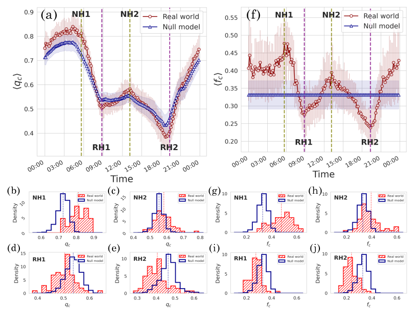
We obtain the percolation threshold $q_{c}(t)$ at a given time $t$, which quantifies the global efficiency of the Seoul traffic flow network at that time, by removing the links from the network based on their quality. The detailed procedure of the percolation process is described in Sec. II.2. Fig. 2(a) shows the intra-day fluctuations in the average percolation threshold, $\langle q_{c}(t)\rangle$, of the Seoul traffic flow network (empty circle symbols). The average value $\langle q_{c}(t)\rangle$ for a given time $t$ is obtained by averaging the percolation thresholds of 57 workdays. Roughly speaking, the value of $\langle q_{c}(t)\rangle$ is very high from 0:00 a.m. to 6:00 a.m., but it decreases rapidly from 6:00 a.m. to 9:00 a.m. It slightly recovers from 9:00 a.m. to 1:00 p.m., declines from 1:00 p.m. to 7:00 p.m., and rapidly recovers after 7:00 p.m. Similar patterns were observed in Beijing, although the values of $q_{c}(t)$ in the morning rush hour tend to be lower than the values in the evening rush hour in the case of Beijing Li et al. (2015). However, it is not clear what makes the observed fluctuating patterns in the global efficiency of the real-world traffic flow networks in Seoul and Beijing.

To identify the effect of the spatial structure of traffic flow networks on their global efficiency, we compare the Seoul traffic flow network with its corresponding null-model network with the same link quality distribution but with a randomly shuffled structure at each time. The detailed procedure for generating the null-model network is described in Sec. II.2. As depicted in Fig. 2(a), the average critical threshold $\langle q_{c}(t)\rangle$ of the Seoul traffic flow network is lower than that of its null model during rush hour (e.g., from 8:00 a.m. to 11:25 a.m. and from 4:10 p.m. to 8:45 p.m.), whereas higher during non-rush hour (e.g., from 11:25 a.m. to 4:10 p.m. and from 8:45 p.m. to 8:00 a.m.). Due to the large standard deviation in the average thresholds, we estimate the distribution of the percolation threshold $q_{c}(t)$ at 5:40 a.m. (Fig. 2(b)), 1:10 p.m. (Fig. 2(c)), 8:50 a.m. (Fig. 2(d)), and 7:20 p.m. (Fig. 2(e)). These distributions support the observation that the Seoul traffic flow network tends to be globally less efficient than its null-model network during rush hour, but more efficient during non-rush hour, indicating that there are qualitatively different efficiency states in the Seoul traffic flow network depending on its spatial structure.

To address the difference in the spatial structure of the real-world networks during rush hour and non-rush hour, first we check the critical removal fraction, $f_{c}(t)$, which represents the fraction of removed links when the percolation process based on link quality reaches the percolation threshold at time $t$. In other words, the critical removal fraction $f_{c}(t)$ is the ratio of the links in the network whose qualities are equal to or lower than $q_{c}(t)$. The time series of the average critical removal fraction, $\langle f_{c}(t)\rangle$, is depicted in Fig. 2(f). Note that $\langle f_{c}(t)\rangle$ of the null-model network appears to be constant because the percolation process is equivalent to random percolation as the link quality is randomly distributed in the network. The average removal fraction $\langle f_{c}(t)\rangle$ of the Seoul traffic flow network is lower than that of its null model during rush hour, while higher during non-rush hour. We also estimate the distribution of the critical removal fraction $f_{c}(t)$ at 5:40 a.m. (Fig. 2(g)) and 1:10 p.m. (Fig. 2(h)), 8:50 a.m. (Fig. 2(i)), and 7:20 p.m. (Fig. 2(j)). These results show that, when we remove low quality links from the real-world network, the smaller fraction of link removal is sufficient to break the network compared to the null model during rush hour, but the larger fraction of link removal is necessary during non-rush hour. This indicates that the quality of links that are important to keep the real-world network connected tends to be lower than the quality of other links during rush hour, but higher during non-rush hour.

Then which links are more important for the global connectivity of a given network? A possible answer would be links with high edge betweenness (EB) Akbarzadeh et al. (2019); Akbarzadeh and Estrada (2018). Since the EB of a link quantifies the number of shortest paths that run along the edge Girvan and Newman (2002), links with high EB of a given network are expected to act as bridges that connect the entire network. Links with EB in the Seoul traffic flow network are depicted in Fig. 3(a). Note that we obtained the EB of each link based on the unweighted version of the Seoul traffic flow network, whose topology is equivalent to the topology of the underlying road network. High EB links tend to be located at the center of the network and have a structure spanning the entire network, whereas low EB links are clustered, localized, and located at the periphery of the network. Hence we can hypothesize that these high EB links are important for keeping the whole network connected. To verify the above hypothesis, we performed a numerical experiment, which removes links from the Seoul traffic flow network in three specific orders: (i) ascending order of EB (i.e., from the lowest to the highest), (ii) random order, and (iii) descending order of EB (i.e., from the highest to the lowest). Figs. 3 (b) and (c) show that, when we remove links with descending order of EB, the critical removal fraction is $f_{c}=0.164$, which is much lower than the critical removal fraction of $f_{c}=0.33$ in the case of random link removal. On the other hand, if we remove links with ascending order of EB, the critical fraction is estimated to be a very high value of $f_{c}=0.958$, indicating that there is virtually no dramatic fragmentation of the GC. The numerical experiment indicates that links with high (low) EB are more (less) important to keep the real-world network connected.

To check whether the highest EB links are more prone to congestion during rush hour than other links, we measure the probability $P(t)$ for each link that the link’s quality is below the critical percolation threshold $q_{c}(t)$ among 57 working days (and thus, the link is removed before the network breaks during the percolation process) at each time $t$. Fig. 4 shows the obtained probabilities averaged over links with a specific range of EB during the day. As shown in Fig. 4(a), top $0-1.6\%$ EB links are much more likely to have lower quality than $q_{c}(t)$ than other links during rush hour. For example, at 6 p.m., $P(t)$ is almost $0.6$ for top $0-0.8\%$ EB links, whereas $f_{c}=0.2702$, indicating that top $0-0.8\%$ EB links are more than twice as likely as all other links to have qualities below $q_{c}$. Moreover, we shuffled the qualities of top $0-1.6\%$ EB links and found that there is no change in $q_{c}$ and $f_{c}$, indicating that congestion of the top EB links still have a strong impact on the network efficiency even if not all of the top EB links are congested. Top $1.6-2.4\%$ EB links show higher $P(t)$ during the morning rush hour but not quite higher $P(t)$ during the evening rush hour. Top $2.4-4.0\%$ EB links show higher $P(t)$ during the evening rush hour but even lower $P(t)$ during the morning rush hour. These results indicate that the highest EB links tend to have lower quality during rush hour compared to links with lower EB, but higher quality during non-rush hour. Fig. 4(b) and (c) show the $P(t)$ of the intermediate EB links and the lowest EB links, respectively. The lowest EB links tend to have $P(t)$ similar to the average during rush hour, but significantly higher $P(t)$ (i.e., their qualities are relatively low) during non-rush hour. Such a difference in the spatial structure leads to the difference in the global efficiency of the real-world traffic flow network.

Finally, we consider two additional topological properties of links to explore whether there is a topological property better than EB: edge degree Holme et al. (2002) and tie range Park, Blumenstock, and Macy (2018). Note that links, edges, and ties are equivalent terms in this article. The degree of an edge connecting node $i$ and $j$ can be defined as: (i) $k_{i}k_{j}$ or (ii) $k_{i}+k_{j}$, where $k_{i}$ is the sum of in-degree and out-degree of node $i$. Tie range is defined as the second-shortest path length, i.e., the number of intermediary ties required to reach from a node to its neighbor if their direct tie are removed. We consider these properties because they quantify how much a given link contributes to the network connectivity. Both properties, however, do not perform better than EB in our data. Although this result does not rule out all other possibilities, we think that EB is an effective topological property for our analysis.

To identify an empirical relation between the network structure and function of urban traffic flows, we analyzed a time-varying real-world traffic flow network and its null-model network with a quality-based percolation method and observed that the real-world network is less efficient than the null model during rush hour, whereas more efficient during non-rush hour. We demonstrate that a difference in the spatial structure of the real-world network during rush hour and non-rush hour is that the quality of the highest EB links is lower than other links during rush hour but higher during non-rush hour, resulting in the difference in the global efficiency.

Our results indicate that urban traffic congestion may not be caused by all traffic flows on the road network being similarly congested, but rather by congestion on parts of the road network that are critical for connecting the whole flow network together. This suggests that these backbone flows and the underlying roads should be considered first when planning urban traffic congestion measures. In the Seoul traffic flow networks, the highest EB links tend to be flows on the highways although there are some exceptions. A recent work also suggests that highways are a key to determine the nature of the percolation transition in urban traffic networks Zeng et al. (2019). Currently, many cities, including Seoul SMG ; TOP , use citywide or city center average speeds as an indication of how well urban traffic flows are working Llorca et al. (2010); He et al. (2016); Rahman et al. (2022), but our research shows that this can be misleading because such average speeds overlook the spatial structure of local traffic flows. We believe that our network approach can provide richer information about how urban traffic flows function.

The data that support the findings of this study are available from the Seoul metropolitan government. Restrictions apply to the availability of these data, which were used under license for this study. Data are available from the authors upon reasonable request and with the permission of the Seoul metropolitan government.

References

- Newman (2018) M. E. J. Newman, Networks, 2nd ed. (Oxford University Press, Oxford, United Kingdom ; New York, NY, United States of America, 2018).
- Barabási and Pósfai (2016) A.-L. Barabási and M. Pósfai, Network Science (Cambridge University Press, Cambridge, 2016).
- Holovatch, Kenna, and Thurner (2017) Y. Holovatch, R. Kenna, and S. Thurner, “Complex systems: physics beyond physics,” European Journal of Physics 38, 023002 (2017).
- Pastor-Satorras and Vespignani (2001) R. Pastor-Satorras and A. Vespignani, “Epidemic spreading in scale-free networks,” Physical Review Letters 86, 3200 (2001).
- Pastor-Satorras et al. (2015) R. Pastor-Satorras, C. Castellano, P. Van Mieghem, and A. Vespignani, “Epidemic processes in complex networks,” Reviews of Modern Physics 87, 925 (2015).
- Albert, Jeong, and Barabasi (2000) R. Albert, H. Jeong, and A.-L. Barabasi, “Error and attack tolerance of complex networks,” Nature 406, 378–382 (2000).
- Callaway et al. (2000) D. S. Callaway, M. E. J. Newman, S. H. Strogatz, and D. J. Watts, “Network robustness and fragility: Percolation on random graphs,” Physical Review Letters 85, 5468 (2000).
- De Martino et al. (2009) D. De Martino, L. Dall’Asta, G. Bianconi, and M. Marsili, “Congestion phenomena on complex networks,” Physical Review E 79, 015101 (2009).
- Zhao et al. (2005) L. Zhao, Y.-C. Lai, K. Park, and N. Ye, “Onset of traffic congestion in complex networks,” Physical Review E 71, 026125 (2005).
- Tan et al. (2014) F. Tan, J. Wu, Y. Xia, and K. T. Chi, “Traffic congestion in interconnected complex networks,” Physical Review E 89, 062813 (2014).
- Solé-Ribalta, Gómez, and Arenas (2016) A. Solé-Ribalta, S. Gómez, and A. Arenas, “Congestion induced by the structure of multiplex networks,” Physical Review Letters 116, 108701 (2016).
- Çolak, Lima, and González (2016) S. Çolak, A. Lima, and M. C. González, “Understanding congested travel in urban areas,” Nature Communications 7, 10793 (2016).
- Olmos et al. (2018) L. E. Olmos, S. Çolak, S. Shafiei, M. Saberi, and M. C. González, “Macroscopic dynamics and the collapse of urban traffic,” Proceedings of the National Academy of Sciences 115, 12654–12661 (2018).
- Rosenlund et al. (2008) M. Rosenlund, F. Forastiere, M. Stafoggia, D. Porta, M. Perucci, A. Ranzi, F. Nussio, and C. A. Perucci, “Comparison of regression models with land-use and emissions data to predict the spatial distribution of traffic-related air pollution in rome,” Journal of Exposure Science & Environmental Epidemiology 18, 192–199 (2008).
- Zhang and Batterman (2013) K. Zhang and S. Batterman, “Air pollution and health risks due to vehicle traffic,” Science of the Total Environment 450, 307–316 (2013).
- Weisbrod, Vary, and Treyz (2003) G. Weisbrod, D. Vary, and G. Treyz, “Measuring economic costs of urban traffic congestion to business,” Transportation Research Record 1839, 98–106 (2003).
- Sweet (2014) M. Sweet, “Traffic congestion’s economic impacts: Evidence from us metropolitan regions,” Urban Studies 51, 2088–2110 (2014).
- Hennessy and Wiesenthal (1999) D. A. Hennessy and D. L. Wiesenthal, “Traffic congestion, driver stress, and driver aggression,” Aggressive Behavior: Official Journal of the International Society for Research on Aggression 25, 409–423 (1999).
- Li et al. (2015) D. Li, B. Fu, Y. Wang, G. Lu, Y. Berezin, H. E. Stanley, and S. Havlin, “Percolation transition in dynamical traffic network with evolving critical bottlenecks,” Proceedings of the National Academy of Sciences 112, 669–672 (2015).
- Zeng et al. (2019) G. Zeng, D. Li, S. Guo, L. Gao, Z. Gao, H. E. Stanley, and S. Havlin, “Switch between critical percolation modes in city traffic dynamics,” Proceedings of the National Academy of Sciences 116, 23–28 (2019).
- Zeng et al. (2020) G. Zeng, J. Gao, L. Shekhtman, S. Guo, W. Lv, J. Wu, H. Liu, O. Levy, D. Li, Z. Gao, et al., “Multiple metastable network states in urban traffic,” Proceedings of the National Academy of Sciences 117, 17528–17534 (2020).
- Ruan et al. (2019) Z. Ruan, C. Song, X.-H. Yang, G. Shen, and Z. Liu, “Empirical analysis of urban road traffic network: A case study in hangzhou city, china,” Physica A: Statistical Mechanics and its Applications 527, 121287 (2019).
- Zhang et al. (2017) L. Zhang, G. Zeng, S. Guo, D. Li, and Z. Gao, “Comparison of traffic reliability index with real traffic data,” EPJ Data Science 6, 1–15 (2017).
- Hamedmoghadam-Rafati et al. (2017) H. Hamedmoghadam-Rafati, I. Steponavice, M. Ramezani, and M. Saberi, “A complex network analysis of macroscopic structure of taxi trips,” IFAC-PapersOnLine 50, 9432–9437 (2017).
- Taillanter and Barthelemy (2021) E. Taillanter and M. Barthelemy, “Empirical evidence for a jamming transition in urban traffic,” Journal of the Royal Society Interface 18, 20210391 (2021).
- Berezin et al. (2015) Y. Berezin, A. Bashan, M. M. Danziger, D. Li, and S. Havlin, “Localized attacks on spatially embedded networks with dependencies,” Scientific Reports 5, 1–5 (2015).
- Hamedmoghadam et al. (2022) H. Hamedmoghadam, N. Zheng, D. Li, and H. L. Vu, “Percolation-based dynamic perimeter control for mitigating congestion propagation in urban road networks,” Transportation Research Part C: Emerging Technologies 145, 103922 (2022).
- Gao et al. (2022) S. Gao, D. Li, N. Zheng, R. Hu, and Z. She, “Resilient perimeter control for hyper-congested two-region networks with mfd dynamics,” Transportation Research Part B: Methodological 156, 50–75 (2022).
- Louf and Barthelemy (2013) R. Louf and M. Barthelemy, “Modeling the polycentric transition of cities,” Physical Review Letters 111, 198702 (2013).
- Louf and Barthelemy (2014) R. Louf and M. Barthelemy, “How congestion shapes cities: from mobility patterns to scaling,” Scientific Reports 4, 5561 (2014).
- Hamedmoghadam et al. (2021) H. Hamedmoghadam, M. Jalili, H. L. Vu, and L. Stone, “Percolation of heterogeneous flows uncovers the bottlenecks of infrastructure networks,” Nature Communications 12, 1–10 (2021).
- Cogoni and Busonera (2021) M. Cogoni and G. Busonera, “Stability of traffic breakup patterns in urban networks,” Physical Review E 104, L012301 (2021).
- Freeman (1977) L. C. Freeman, “A set of measures of centrality based on betweenness,” Sociometry , 35–41 (1977).
- Girvan and Newman (2002) M. Girvan and M. E. Newman, “Community structure in social and biological networks,” Proceedings of the National Academy of Sciences 99, 7821–7826 (2002).
- Newman (2012) M. E. Newman, “Communities, modules and large-scale structure in networks,” Nature Physics 8, 25–31 (2012).
- Wang et al. (2022) F. Wang, G. Dong, L. Tian, and H. E. Stanley, “Percolation behaviors of finite components on complex networks,” New Journal of Physics 24, 043027 (2022).
- Hébert-Dufresne and Allard (2019) L. Hébert-Dufresne and A. Allard, “Smeared phase transitions in percolation on real complex networks,” Physical Review Research 1, 013009 (2019).
- Li et al. (2021) M. Li, R.-R. Liu, L. Lü, M.-B. Hu, S. Xu, and Y.-C. Zhang, “Percolation on complex networks: Theory and application,” Physics Reports 907, 1–68 (2021).
- Akbarzadeh et al. (2019) M. Akbarzadeh, S. Memarmontazerin, S. Derrible, and S. F. Salehi Reihani, “The role of travel demand and network centrality on the connectivity and resilience of an urban street system,” Transportation 46, 1127–1141 (2019).
- Akbarzadeh and Estrada (2018) M. Akbarzadeh and E. Estrada, “Communicability geometry captures traffic flows in cities,” Nature human behaviour 2, 645–652 (2018).
- Holme et al. (2002) P. Holme, B. J. Kim, C. N. Yoon, and S. K. Han, “Attack vulnerability of complex networks,” Physical review E 65, 056109 (2002).
- Park, Blumenstock, and Macy (2018) P. S. Park, J. E. Blumenstock, and M. W. Macy, “The strength of long-range ties in population-scale social networks,” Science 362, 1410–1413 (2018).
- (43) “Seoul Metropolitan Government,” https://data.seoul.go.kr/, 2020.
- (44) “Seoul Transport Operation and Information Services,” https://topis.seoul.go.kr/, 2020.
- Llorca et al. (2010) D. F. Llorca, M. Sotelo, S. Sánchez, M. Ocaña, J. Rodríguez-Ascariz, and M. García-Garrido, “Traffic data collection for floating car data enhancement in v2i networks,” EURASIP Journal on Advances in Signal Processing 2010, 1–13 (2010).
- He et al. (2016) F. He, X. Yan, Y. Liu, and L. Ma, “A traffic congestion assessment method for urban road networks based on speed performance index,” Procedia Engineering 137, 425–433 (2016).
- Rahman et al. (2022) M. M. Rahman, P. Najaf, M. G. Fields, and J.-C. Thill, “Traffic congestion and its urban scale factors: Empirical evidence from american urban areas,” International Journal of Sustainable Transportation 16, 406–421 (2022).