This paper was converted on www.awesomepapers.org from LaTeX by an anonymous user.
Want to know more? Visit the Converter page.

Global Bifurcation of Non-Radial Solutions for Symmetric Sub-linear Elliptic Systems on the Planar Unit Disc

Ziad Ghanem Department of Mathematical Sciences, University of Texas at Dallas, Richardson, TX 75080, USA [email protected] Casey Crane Department of Mathematical Sciences, University of Texas at Dallas, Richardson, TX 75080, USA [email protected]  and  Jingzhou Liu Department of Mathematical Sciences, University of Texas at Dallas, Richardson, TX 75080, USA [email protected]
Abstract.

In this paper, we prove a global bifurcation result for the existence of non-radial branches of solutions to the paramterized family of Γ\Gamma-symmetric equations Δu=f(α,z,u)-\Delta u=f(\alpha,z,u), u|D=0u|_{\partial D}=0 on the unit disc D:={z:|z|<1}D:=\{z\in{\mathbb{C}}:|z|<1\} with u(z)ku(z)\in\mathbb{R}^{k}, where k\mathbb{R}^{k} is an orthogonal Γ\Gamma-representation, f:×D¯×kkf:\mathbb{R}\times\overline{D}\times\mathbb{R}^{k}\to\mathbb{R}^{k} is a sub-linear Γ\Gamma-equivariant continuous function, differentiable with respect to uu at zero and satisfying the conditions f(α,eiθz,u)=f(α,z,u)f(\alpha,e^{i\theta}z,u)=f(\alpha,z,u) for all θ\theta\in\mathbb{R} and f(z,u)=f(z,u)f(z,-u)=-f(z,u).

Mathematics Subject Classification: Primary: 37G40, 35B06; Secondary: 47H11, 35J57, 35J91, 35B32, 47J15

Key Words and Phrases: global bifurcation, non-linear Laplace equation, symmetric bifurcation, bifurcation invariant, non-radial solutions, equivariant Brouwer degree.

1. Introduction

We draw our motivation from natural phenomena that are modeled by parameterized systems of autonomous Partial Differential Equations (PDEs), where the possible states of each phenomenon are represented by solutions of the associated system of equations at corresponding parameter values. These solutions can be categorized as trivial or non-trivial. Trivial solutions are so-named because they persist for all parameter values and their existence is straightforward to determine. In contrast, non-trivial solutions may only exist for a particular range of parameter values and often exhibit exotic properties that enhance our understanding of the model. The classical bifurcation problem is concerned with the existence and global behaviour of branches of non-trivial solutions emerging from their trivial counterparts. Phenomena which admit the symmetries of a certain group GG (represented by the GG-equivariance of the associated equations) may be studied as equivariant bifurcation problems, with additional consideration placed on the symmetric properties of these branches (cf. [1, 3, 9, 11, 19, 21, 22, 23, 24, 25]). The application of topological methods to the study of differential equations, as with most tools in the arsenal of the nonlinear analyst, traces back to M. Poincare [13]. More recently, the Local/Equivariant Brouwer Degrees and their infinite dimensional generalizations – the Local/Equivariant Leray-Schauder Degrees – have proven prodigiously effective in obtaining existence results for solutions to a wide class of nonlinear differential equations. Somewhat remarkably, these degree theories are also instrumental in solving classical and equivariant bifurcation problems. The first use of the Leray-Schauder degree for the detection of (local) bifurcation in a parameterized system of nonlinear differential equations is attributed to the seminal work of M.A. Krasnosel’skii, in which sufficient conditions for the existence of a branch of non-trivial solutions are established (cf. [17]). Only a decade later, P. Rabinowitz (cf. [20]) proposed his famous Rabinowitz alternative, which provides sufficient conditions for the unboundedness of a branch of non-trivial solutions. In this paper, we employ equivariant analogues of Krasnosel’skii and Rabinowitz type results to solve an equivariant bifurcation problem. Specifically, our objective is to study the equivariant bifurcation problem for a symmetric system of parameterized nonlinear Laplace equations subject to Dirichlet boundary conditions. The bifurcation and global behaviour of solutions for such systems has been extensively studied, due to their significance in applied mathematics and physics. In the case that the nonlinearity arises as the gradient of some potential function, the bifurcation problem can be studied as a parameterized variational problem and appropriate topological methods such as Morse theory, index theory, and the equivariant gradient degree (cf. [14]) can be administered (cf. [6, 7, 8, 10, 12, 11, 21, 22, 23, 24, 25, 26]). However, these approaches are not applicable for systems which lack variational structure. The degree theoretic methods used in this paper impose no variational requirements on the equations and, as such, are broadly applicable to a wider class of problems. Consider the following parameterized family of symmetric Laplace equations:

(1) {Δu=f(α,z,u),α,zD,u(z)Vu|D=0,\begin{cases}-\Delta u=f(\alpha,z,u),\quad\alpha\in\mathbb{R},\;z\in D,\;u(z)\in V\\ u|_{\partial D}=0,\end{cases}

where D:={z:|z|<1}D:=\{z\in{\mathbb{C}}:|z|<1\} is the unit planar disc, V:=kV:=\mathbb{R}^{k} is an orthogonal representation of a finite group Γ\Gamma and f:×D¯×VVf:\mathbb{R}\times\overline{D}\times V\to V is a continuous, odd, radially symmetric and Γ\Gamma-equivariant family of functions of sub-linear growth, which are differentiable with respect to uu at the origin in VV. In particular, we assume that ff satisfies the following conditions:

  1. (A1A_{1})

    f(α,eiθz,u)=f(α,z,u)f(\alpha,e^{i\theta}z,u)=f(\alpha,z,u)   for all α,zD\alpha\in\mathbb{R},\;z\in D,   uVu\in V and θ\theta\in\mathbb{R};

  2. (A2A_{2})

    f(α,z,γu)=γf(α,z,u)f(\alpha,z,\gamma u)=\gamma f(\alpha,z,u)   for all α,zD\alpha\in\mathbb{R},\;z\in D,   uVu\in V and γΓ\gamma\in\Gamma;

  3. (A3A_{3})

    f(α,z,u)=f(α,z,u)f(\alpha,z,-u)=-f(\alpha,z,u)   for all α\alpha\in\mathbb{R},   zDz\in D and uVu\in V;

  4. (A4A_{4})

    there exist continuous functions A:L(k,)A:\mathbb{R}\to L(k,\mathbb{R}), c:(0,)c:\mathbb{R}\rightarrow(0,\infty) and a number β>1\beta>1 such that for each α\alpha\in\mathbb{R} one has

    |f(α,z,u)A(α)u|c(α)|u|βfor allzD¯,uV;\displaystyle|f(\alpha,z,u)-A(\alpha)u|\leq c(\alpha)|u|^{\beta}\quad\text{for all}\;{z\in\overline{D}},\;{u\in V};
  5. (A5A_{5})

    there exist continuous functions a,b:(0,)a,b:\mathbb{R}\rightarrow(0,\infty) and a number ν(0,1)\nu\in(0,1) such that for each α\alpha\in\mathbb{R} the following inequality holds

    |f(α,z,u)|<a(α)|u|ν+b(α)for allzD¯,uV.\displaystyle|f(\alpha,z,u)|<a(\alpha)|u|^{\nu}+b(\alpha)\quad\text{for all}\;{z\in\overline{D}},{u\in V}.

Conditions (A1A_{1}) (A2A_{2}) and (A3A_{3}) imply the O(2)×Γ×2O(2)\times\Gamma\times\mathbb{Z}_{2}-symmetry of system (1) in the sense that f:×D¯×VVf:\mathbb{R}\times\overline{D}\times V\to V is O(2)O(2)-invariant with respect to the O(2)O(2)-action O(2)×DDO(2)\times D\rightarrow D given by (θ,z)eiθz(\theta,z)\rightarrow e^{i\theta}z, (κ,z)z¯(\kappa,z)\rightarrow\overline{z} and Γ×2\Gamma\times\mathbb{Z}_{2}-equivariant with respect to the Γ×2\Gamma\times\mathbb{Z}_{2} action (Γ×2)×VV(\Gamma\times\mathbb{Z}_{2})\times V\rightarrow V given by (γ,±1,u)±γu(\gamma,\pm 1,u)\rightarrow\pm\gamma u. On the other hand, conditions (A4A_{4}) and (A5A_{5}) guarantee differentiability at the origin and sublinearity, respectively.

Remark 1.1.

Since the zero function is a solution to (1) for all values α\alpha\in\mathbb{R}, all trivial solutions to the system are of the form (α,0)(\alpha,0). Non-trivial solutions to (1), on the other hand, fall into two categories, namely:

  • (i)

    radial solutions, which depend only on the magnitude |z||z| of any disc element zDz\in D (although less obvious than the trivial solution, radial solutions can often be identified using classical methods, eg. by reducing (1) to a second order ODE);

  • (ii)

    and non-radial solutions, which exhibit dependency on the angular variable.

Our objective is to identify branches of non-radial solutions to (1), describe their possible symmetric properties, and characterize their global behavior.

The methods used in this paper are inspired by [2], where an existence result was obtained for a similar sublinear elliptic system using equivariant degree theory. For a more thorough exposition of these topics, we direct readers to the recent monograph [4] or, alternatively, the older text [5]. The equivariant degree is intimately connected with the classical Brouwer degree. Although its application is relatively simple, technical difficulties arise when dealing with algebraic computations related to unfamiliar group structures. Many of these issues can be resolved with usage of the G.A.P. system, and the G.A.P. package EquiDeg (created by Haopin Wu), which is available online at https://github.com/psistwu/equideg (cf. [28]). In the remainder of this paper, we employ tools from the equivariant degree theory to determine (i)(i) under what conditions branches of non-trivial solutions may bifurcate from a trivial solution, (ii)(ii) under what conditions these branches consist only of non-radial solutions and (iii)(iii) under what conditions these branches are unbounded. Subsequent sections are organized as follows: In Section 2 the problem (1) is reformulated in an appropriate functional setting. In Section 3 we recall the abstract equivariant bifurcation results, including the equivariant analogues of the classical Krasnosel’skii and Rabinowitz theorems. In Section 4, we apply the equivariant degree theory methods to establish local and global bifurcation results for (1). Finally, in Section 5 we present a motivating example of vibrating membranes where our main results, Theorem 4.1 and 4.3, are applied to demonstrate the existence of unbounded branches of non-radial solutions admitting all possible maximal orbit types. For convenience, the Appendices include an explanation of notations used, a summary of the spectral properties of the Laplace operator on the unit disc, and a brief introduction to the Brouwer equivariant degree theory. Acknowledgment: We are deeply grateful to our advisor, Professor Krawcewicz, whose invaluable guidance and unwavering support made this work possible. We would also like to acknowledge Professor Garcia-Azpetia for insightful discussions regarding the estimation of the behaviour of our system near a bifurcation point.

2. Functional Space Reformulation and a priori Bounds

Consider the Sobolev space :=H2(D,V)H01(D,V)\mathscr{H}:=H^{2}(D,V)\cap H^{1}_{0}(D,V) equipped with the usual norm

u:=max{Dsu2:|s|2},\displaystyle\|u\|_{\mathscr{H}}:=\max\{\|D^{s}u\|_{2}:|s|\leq 2\},

where s:=(s1,s2)s:=(s_{1},s_{2}), |s|:=s1+s22|s|:=s_{1}+s_{2}\leq 2, and Dsφ:=|s|φs1xs2yD^{s}\varphi:=\frac{\partial^{|s|}\varphi}{\partial^{s_{1}}x\partial^{s_{2}}y}. It is well known that the Laplacian operator :L2(D,V)\mathscr{L}:\mathscr{H}\to L^{2}(D,V) given by

(2) u:=Δu,\displaystyle\mathscr{L}u:=-\Delta u,

is a linear isomorphism. Let ν(0,1)\nu\in(0,1) be the scalar from condition (A5A_{5}). If one chooses q>max{1,2ν}q>\max\{1,2\nu\} (for example, it is enough to take q:=2βq:=2\beta (cf. assumption (A4A_{4})), then there is the standard Sobolev embedding j:Lq(D,V)j:\mathscr{H}\to L^{q}(D,V)

(3) j(u)(z):=u(z),u,j(u)(z):=u(z),\quad u\in\mathscr{H},

and also its associated Nemytski operator Nα:Lq(D,V)L2(D,V)N_{\alpha}:L^{q}(D,V)\rightarrow L^{2}(D,V)

(4) Nα(v)(z):=f(α,z,v(z)),zD,α.N_{\alpha}(v)(z):=f(\alpha,z,v(z)),\quad z\in D,\;\alpha\in\mathbb{R}.
Lemma 2.1.

Under conditions (A1A_{1})(A5A_{5}), The Nemystiki operator (4) is well-defined.

Proof.

It suffices to demonstrate that for any vLq(D,V)v\in L^{q}(D,V) and α\alpha\in\mathbb{R} one has Nα(v)L2(D,V)N_{\alpha}(v)\in L^{2}(D,V). Combining (A5A_{5}) with the Hölder inequality, one has:

Nα(v)L2\displaystyle\|N_{\alpha}(v)\|_{L^{2}} =f(α,z,v)L2\displaystyle=\|f(\alpha,z,v)\|_{L^{2}}
a(α)|v|νL2+b(α)L2\displaystyle\leq\|\,a(\alpha)|v|^{\nu}\|_{L^{2}}+\|\,b(\alpha)\|_{L^{2}}
=a(α)|v|νL2+b(α)π\displaystyle=a(\alpha)\|\,|v|^{\nu}\|_{L^{2}}+b(\alpha)\sqrt{\pi}
=a(α)(D|v|2ν)12+b(α)π\displaystyle=a(\alpha)\left(\int_{D}|v|^{2\nu}\right)^{\frac{1}{2}}+b(\alpha)\sqrt{\pi}
a(α)π12ν/q2(D|v|2νq2ν)2ν2q+b(α)π\displaystyle\leq a(\alpha)\pi^{{1-2\nu/q}\over 2}\left(\int_{D}|v|^{\frac{2\nu q}{2\nu}}\right)^{\frac{2\nu}{2q}}+b(\alpha)\sqrt{\pi}
(5) =a(α)π1/2ν/qvLqν+b(α)π,\displaystyle=a(\alpha)\pi^{1/2-\nu/q}\|v\|^{\nu}_{L^{q}}+b(\alpha)\sqrt{\pi},

where the result follows from b(α),a(α),vq<b(\alpha),a(\alpha),\|v\|_{q}<\infty. \square Notice that the equation

(6) u=Nα(ju),α,u,\mathscr{L}u=N_{\alpha}(ju),\quad\alpha\in\mathbb{R},u\in\mathscr{H},

is equivalent to system (1) in the sense that uu\in\mathscr{H} is a solution to (1) for some α\alpha\in\mathbb{R} if and only if (α,u)×(\alpha,u)\in\mathbb{R}\times\mathscr{H} satisfies (6). In turn, the invertibility of \mathscr{L} together with Lemma (2.1) imply that the map :×\mathscr{F}:\mathbb{R}\times\mathscr{H}\to\mathscr{H} given by

(7) (α,u):=u1Nα(ju),\mathscr{F}(\alpha,u):=u-\mathscr{L}^{-1}N_{\alpha}(ju),

is well-defined. Hence, system (1) is also equivalent to the equation

(8) (α,u)=0,α,u.\mathscr{F}(\alpha,u)=0,\quad\alpha\in\mathbb{R},\;u\in\mathscr{H}.

In what follows, we will call (8) the operator equation associated with (1).

Lemma 2.2.

Let f:×D¯×VVf:\mathbb{R}\times\overline{D}\times V\rightarrow V be a continuous function satisfying the assumption (A5A_{5}). For every α\alpha\in\mathbb{R}, there exists a constant R(α)>0R(\alpha)>0 such that, if (α,u)×(\alpha,u)\in\mathbb{R}\times\mathscr{H} is a solution to system (1), then u<R(α)\|u\|_{\mathscr{H}}<R(\alpha).

Proof.

Assume that (α,u)×(\alpha,u)\in\mathbb{R}\times\mathscr{H} is a solution to system (1). Combining (5) with u=1Nα(ju)u=\mathscr{L}^{-1}N_{\alpha}(ju), one has

(9) ua(α)π1/2ν/q1uL2ν+b(α)π1,\|u\|_{\mathscr{H}}\leq a(\alpha)\pi^{1/2-\nu/q}\|\mathscr{L}^{-1}\|\,\|u\|_{L_{2}}^{\nu}+b(\alpha)\sqrt{\pi}\|\mathscr{L}^{-1}\|,

which, together with uuL2\|u\|_{\mathscr{H}}\geq\|u\|_{L^{2}}, implies

(10) uL2cuL2ν+d,\displaystyle\|u\|_{L^{2}}\leq c\|u\|^{\nu}_{L^{2}}+d,

where c:=a(α)π1/2ν/q1c:=a(\alpha)\pi^{1/2-\nu/q}\|\mathscr{L}^{-1}\|, d:=b(α)π1d:=b(\alpha)\sqrt{\pi}\|\mathscr{L}^{-1}\|. Finally, since 0<ν<10<\nu<1, there exists R0(α)>0R_{0}(\alpha)>0 such that ψ(t):=tctνd>0\psi(t):=t-ct^{\nu}-d>0 for tR0(α)t\geq R_{0}(\alpha). Consequently, uL2<R0(α)\|u\|_{L^{2}}<R_{0}(\alpha), and by (9),

ucuL2ν+d<cR0(α)ν+d=:R(α)\|u\|_{\mathscr{H}}\leq c\|u\|^{\nu}_{L^{2}}+d<cR_{0}(\alpha)^{\nu}+d=:R(\alpha)

is the required constant. \square

3. Abstract Local and Global Equivariant Bifurcation

In this section we present a concise exposition, following [4] and [5], of an equivariant Brouwer degree method to study symmetric bifurcation problems. Given a compact Lie group 𝒢\mathcal{G}, an isometric Banach 𝒢\mathcal{G}-representation \mathcal{H} and a completely continuous 𝒢\mathcal{G}-equivariant field :×\mathcal{F}:\mathbb{R}\times\mathcal{H}\rightarrow\mathcal{H}, we use the Leray-Schauder Equivariant 𝒢\mathcal{G}-Degree to describe local and global properties of the solution set to the equation,

(11) (α,u)=0,α,u.\mathcal{F}(\alpha,u)=0,\quad\alpha\in\mathbb{R},\;u\in\mathcal{H}.

To simplify our exposition and for compatibility with the system of interest (8), we make the following two assumptions.

  1. (B1B_{1})

    The set of trivial solutions to (11) is given by

    M:={(α,0)×}.\displaystyle M:=\{(\alpha,0)\in\mathbb{R}\times\mathcal{H}\}.
  2. (B2B_{2})

    There exists a continuous family of linear operators 𝒜(α):\mathcal{A}(\alpha):\mathcal{H}\rightarrow\mathcal{H} such that, for every α\alpha\in\mathbb{R}, the derivative Du(α,0)D_{u}\mathcal{F}(\alpha,0) exists and

    𝒜(α):=D(α,0).\displaystyle\mathcal{A}(\alpha):=D\mathcal{F}(\alpha,0).

Solutions to (11) which do not belong to MM are called nontrivial. Let 𝒮1(0)\mathcal{S}\subset\mathcal{F}^{-1}(0) denote the set of all non-trivial solutions, i.e.

𝒮:={(α,u)×:(α,u)=0 and u0}.\mathcal{S}:=\{(\alpha,u)\in\mathbb{R}\times\mathcal{H}\;:\;\mathcal{F}(\alpha,u)=0\text{ and }u\neq 0\}.

Clearly, the set of non-trivial solutions 𝒮×\mathcal{S}\subset\mathbb{R}\times\mathcal{H} is 𝒢\mathcal{G}-invariant.

3.1. The Local Bifurcation Invariant and Krasnosel’skii’s Theorem

Formulation of a Krasnosel’skii type local bifurcation result for equation (11) necessitates the introduction of additional notations and terminology (for more details, the reader is referred to [1, 4]). Our first definition clarifies what is meant by a bifurcation of the equation (11).

Definition 3.1.

A trivial solution (α0,0)M(\alpha_{0},0)\in M is said to be a bifurcation point for the equation (11) if every open neighborhood of the point (α0,0)(\alpha_{0},0) has non-trivial intersection with 𝒮\mathcal{S}.

It is well-known that a necessary condition for any trivial solution (α0,0)M(\alpha_{0},0)\in M to be a bifurcation point for the equation (11) is that the linear operator 𝒜(α0):\mathcal{A}(\alpha_{0}):\mathcal{H}\rightarrow\mathcal{H} is not an isomorphism. This leads to the following definition.

Definition 3.2.

A trivial solution (α0,0)M(\alpha_{0},0)\in M is said to be a regular point for the equation (11) if 𝒜(α0)\mathcal{A}(\alpha_{0}) is an isomorphism and a critical point otherwise. Moreover, a critical point (α0,0)M(\alpha_{0},0)\in M is said to be isolated if there exists a deleted ϵ\epsilon-neighborhood 0<|αα0|<ϵ0<|\alpha-\alpha_{0}|<\epsilon such that for all α(α0ϵ,α0+ϵ){α0}\alpha\in(\alpha_{0}-\epsilon,\alpha_{0}+\epsilon)\setminus\{\alpha_{0}\}, the point (α,0)M(\alpha,0)\in M is regular.

The set of all critical points for equation (11), denoted Λ\Lambda, is called the critical set, i.e.

(12) Λ:={(α,0): 𝒜(α): is not an isomorphism}.\displaystyle\Lambda:=\{(\alpha,0):\text{ $\mathcal{A}(\alpha):\mathcal{H}\rightarrow\mathcal{H}$ is not an isomorphism}\}.

The next definition concerns our interest in the continuation of non-trivial solution emerging from a bifurcation point (α0,0)M(\alpha_{0},0)\in M.

Definition 3.3.

A trivial solution (α0,0)M(\alpha_{0},0)\in M is said to be a branching point for the equation (11) if there exists a non-trivial continuum KS¯K\subset\overline{S} with KM={(α0,0)}K\cap M=\{(\alpha_{0},0)\} and the maximal connected set 𝒞S¯\mathcal{C}\subset\overline{S} containing the branching point (α0,0)(\alpha_{0},0) we call a branch of nontrivial solutions bifurcating from the point (α0,0)(\alpha_{0},0).

Whereas the classical Krasnosiel’skii bifurcation result is only concerned with the existence of a branch of nontrivial solutions for the equation (11) bifurcating from a given critical point (α0,0)Λ(\alpha_{0},0)\in\Lambda, the equivariant Krasnosiel’skii bifurcation result, which we employ in this paper, is also concerned with the symmetric properties of such a branch.

Definition 3.4.

Given a subgroup H𝒢H\leq\mathcal{G}, denote by 𝒮H\mathcal{S}^{H} the corresponding HH-fixed point space of non-trivial solutions. A branch of solutions 𝒞\mathcal{C} is said to have symmetries at least (H)(H) if 𝒞𝒮H\mathcal{C}\cap\mathcal{S}^{H}\not=\emptyset.

Let (α0,0)Λ(\alpha_{0},0)\in\Lambda be an isolated critical point with a deleted ϵ\epsilon-neighborhood

{α:0<|αα0|<ϵ},\{\alpha\in\mathbb{R}:0<|\alpha-\alpha_{0}|<\epsilon\},

on which 𝒜(α):\mathscr{A}(\alpha):\mathscr{H}\rightarrow\mathscr{H} is an isomorphism and choose α0±(α0ε,α0+ε)\alpha^{\pm}_{0}\in(\alpha_{0}-\varepsilon,\alpha_{0}+\varepsilon) with α0α0α0+\alpha^{-}_{0}\leq\alpha_{0}\leq\alpha^{+}_{0}. Since 𝒜(α±):\mathcal{A}(\alpha^{\pm}):\mathscr{H}\rightarrow\mathscr{H} are non-singular, there exists a number δ>0\delta>0 sufficiently small such that, adopting the notations ±(u):=(α0±,u)\mathcal{F}_{\pm}(u):=\mathcal{F}(\alpha^{\pm}_{0},u), Bδ:={u:u<δ}B_{\delta}:=\{u\in\mathscr{H}:\|u\|<\delta\}, one has

±1(0)Bδ=,\mathcal{F}_{\pm}^{-1}(0)\cap\partial B_{\delta}=\emptyset,

and ±\mathcal{F}_{\pm} are BδB_{\delta}-admissibly 𝒢\mathcal{G}-homotopic to 𝒜(α±)\mathcal{A}(\alpha^{\pm}). Moreover, since 𝒢\mathcal{G} acts isometrically on \mathscr{H}, the ball BδB_{\delta} is clearly 𝒢\mathcal{G}-invariant. It follows, from the homotopy property of the 𝒢\mathcal{G}-equivariant Leray-Schauder degree (cf. Appendix C), that (±,Bδ)(\mathcal{F}_{\pm},B_{\delta}) are admissible 𝒢\mathcal{G}-pairs in \mathscr{H} and also that 𝒢-deg(±,Bδ)=𝒢-deg(𝒜(α0±),B())\mathcal{G}\text{-deg}(\mathcal{F}_{\pm},B_{\delta})=\mathcal{G}\text{-deg}(\mathcal{A}(\alpha^{\pm}_{0}),B(\mathscr{H})), where B()B(\mathscr{H}) is the open unit ball in \mathscr{H}. We call the Burnside Ring element

(13) ω𝒢(α0)=𝒢-deg(𝒜(α0),B())𝒢-deg(𝒜(α0+),B()),\displaystyle\omega_{\mathcal{G}}(\alpha_{0})=\mathcal{G}\text{-deg}(\mathcal{A}(\alpha^{-}_{0}),B(\mathscr{H}))-\mathcal{G}\text{-deg}(\mathcal{A}(\alpha^{+}_{0}),B(\mathscr{H})),

the local bifurcation invariant at (λ0,0)(\lambda_{0},0). The reader is referred to [4] or [5] for proof that the invariant (13) does not depend on the choice of α0±\alpha^{\pm}_{0}\in\mathbb{R} or radius δ>0\delta>0, and also for the proof of the following local bifurcation result, which is a consequence of the equivariant version of a classical result of K. Kuratowski (cf. [18], Thm. 3, p. 170).

Theorem 3.1.

(M.A. Krasnosel’skii-Type Local Bifurcation) Let :×\mathcal{F}:\mathbb{R}\times\mathscr{H}\rightarrow\mathscr{H} be a completely continuous 𝒢\mathcal{G}-equivariant field satisfying the assumptions (B1B_{1}) and (B2B_{2}) and with an isolated critical point (α0,0)(\alpha_{0},0). If ω𝒢(α0)0\omega_{\mathcal{G}}(\alpha_{0})\neq 0, then

  • (i)

    there exists a branch of nontrivial solutions 𝒞\mathcal{C} to system (11) with branching point (α0,0)(\alpha_{0},0);

  • (ii)

    moreover, if (H)Φ0(G)(H)\in\Phi_{0}(G) is an orbit type with

    coeffH(ω𝒢(α0))0,\displaystyle\operatorname{coeff}^{H}(\omega_{\mathcal{G}}(\alpha_{0}))\neq 0,

then there exists a branch of non-trivial solutions bifurcating from (α0,0)(\alpha_{0},0) with symmetries at least (H)(H).

3.2. Global Bifurcation and the Rabinowitz Alternative

In order to employ the Leray-Schauder 𝒢\mathcal{G}-equivariant degree to describe the global properties of a branch of non-trivial solutions bifurcating from an isolated critical point of the equation (11), we need to make an additional assumption.

  1. (B3B_{3})

    The critical set ΛM\Lambda\subset M (given by (12)) is discrete.

Notice that the local bifurcation invariant ω𝒢(α0)\omega_{\mathcal{G}}(\alpha_{0}) at any critical point (α0,0)Λ(\alpha_{0},0)\in\Lambda is well-defined under assumption (B3B_{3}). Moreover, if 𝒰×\mathcal{U}\subset\mathbb{R}\times\mathscr{H} is an open bounded 𝒢\mathcal{G}-invariant set, then its intersection with the critical set is finite. These observations will be important for the statement of the following global bifurcation result, the proof of which can be found in [4], [5].

Theorem 3.2.

(The Rabinowitz Alternative) Suppose that :×\mathcal{F}:\mathbb{R}\times\mathscr{H}\rightarrow\mathscr{H} is a completely continuous 𝒢\mathcal{G}-equivariant field satisfying conditions (B1B_{1})(B3B_{3}) and let 𝒰×\mathcal{U}\subset\mathbb{R}\times\mathscr{H} be an open bounded 𝒢\mathcal{G}-invariant set with 𝒰Λ=\partial\mathcal{U}\cap\Lambda=\emptyset. If 𝒞\mathcal{C} is a branch of nontrivial solutions to (11) bifurcating from the critical point (α0,0)𝒰Λ(\alpha_{0},0)\in\mathcal{U}\cap\Lambda, then one has the following alternative:

  1. (a)(a)

    either 𝒞𝒰\mathcal{C}\cap\partial\mathcal{U}\neq\emptyset;

  2. (b)(b)

    or there exists a finite set

    𝒞Λ={(α0,0),(α1,0),,(αn,0)},\displaystyle\mathcal{C}\cap\Lambda=\{(\alpha_{0},0),(\alpha_{1},0),\ldots,(\alpha_{n},0)\},

    satisfying the following relation

    k=1nω𝒢(αk)=0.\displaystyle\sum\limits_{k=1}^{n}\omega_{\mathcal{G}}(\alpha_{k})=0.
Remark 3.1.

Suppose that Theorem 3.1 is used to demonstrate the existence of a branch 𝒞\mathcal{C} of nontrivial solutions to (11) bifurcating from a critical point (α0,0)(\alpha_{0},0) and that certain conditions are met such that, for any open bounded 𝒢\mathcal{G}-invariant neighborhood 𝒰(α0,0)\mathcal{U}\ni(\alpha_{0},0) with 𝒰Λ=\partial\mathcal{U}\cap\Lambda=\emptyset, the alternative (b)(b) is impossible. Then, according to Theorem 3.2, the branch 𝒞\mathcal{C} must be unbounded.

4. Local and Global Bifurcation of Non-radial Solutions in (1)

Returning to the functional reformulation of our original problem described in Section 2, consider the product group G:=O(2)×Γ×2G:=O(2)\times\Gamma\times\mathbb{Z}_{2} and notice that the Sobolev space \mathscr{H} is a natural Banach GG-representation with respect to the isometric GG-action G×G\times\mathscr{H}\rightarrow\mathscr{H} given by

(14) (θ,γ,±1)u(z)\displaystyle(\theta,\gamma,\pm 1)u(z) :=±γu(eiθz),zD,u;\displaystyle:=\pm\gamma u(e^{i\theta}\cdot z),\quad z\in D,\;\;u\in\mathscr{H};
(κ,γ,±1)u(z)\displaystyle(\kappa,\gamma,\pm 1)u(z) :=±γu(z¯),γΓ,κO(2),θSO(2),\displaystyle:=\pm\gamma u(\overline{z}),\quad\gamma\in\Gamma,\;\kappa\in O(2),\;\theta\in SO(2),

where z¯\overline{z} is the complex conjugation of zDz\in D and eiθze^{i\theta}\cdot z is the standard complex multiplication.

Remark 4.1.

Under assumptions (A1A_{1})-(A5A_{5}), the nonlinear operator :×\mathscr{F}:\mathbb{R}\times\mathscr{H}\rightarrow\mathscr{H} given by (7) is a completely continuous GG-equivariant field, differentiable at 00\in\mathscr{H} with

D(α,0)=Id1A(α):,\displaystyle D\mathscr{F}(\alpha,0)=\operatorname{Id}-\mathscr{L}^{-1}A(\alpha):\mathscr{H}\rightarrow\mathscr{H},

where A(α):VVA(\alpha):V\rightarrow V is the linearization of the map f(α,z,u)f(\alpha,z,u) from the equation (1) at the origin (see for example see [16, 2]). For convenience, we introduce the notation

(15) 𝒜(α)(u):=u1A(α)u,u.\mathscr{A}(\alpha)(u):=u-\mathscr{L}^{-1}A(\alpha)u,\quad u\in\mathscr{H}.

Before approaching the question of bifurcation in the equation (1), we must derive a workable formula for the computation of the degree G-deg(𝒜(α),B())G\text{\rm-deg}(\mathscr{A}(\alpha),B(\mathscr{H})), where B():={u:u<1}B(\mathscr{H}):=\{u\in\mathscr{H}:\|u\|_{\mathscr{H}}<1\} is the open unit ball in \mathscr{H} and α\alpha\in\mathbb{R} is any parameter value for which 𝒜(α):\mathscr{A}(\alpha):\mathscr{H}\rightarrow\mathscr{H} is an isomorphism. Assuming that a complete list of the irreducible Γ\Gamma-representations {𝒱j}j=1r\{\mathcal{V}_{j}\}_{j=1}^{r} is made available we denote by {𝒱j}j=1r\{\mathcal{V}_{j}^{-}\}_{j=1}^{r} the corresponding list of irreducible Γ×2\Gamma\times\mathbb{Z}_{2}-representations, where the superscript is meant to indicate that each irreducible Γ\Gamma-representation has been equipped with the antipodal 2\mathbb{Z}_{2}-action in the standard way (cf. [4], [5]). As a Γ\Gamma-representation, V=kV=\mathbb{R}^{k} is also a natural Γ×2\Gamma\times\mathbb{Z}_{2}-representation with the Γ×2\Gamma\times\mathbb{Z}_{2}-isotypic decomposition

V=V1V2Vr,\displaystyle V=V_{1}\oplus V_{2}\oplus\cdots\oplus V_{r},

where each Γ×2\Gamma\times\mathbb{Z}_{2}-isotypic component component VjV_{j} is modeled on the irreducible Γ×2\Gamma\times\mathbb{Z}_{2}-representation 𝒱j\mathcal{V}_{j}^{-} in the sense that VjV_{j} is equivalent to the direct sum of some number of copies of 𝒱j\mathcal{V}_{j}^{-}, i.e.

Vj𝒱j𝒱j.\displaystyle V_{j}\simeq\mathcal{V}_{j}^{-}\oplus\cdots\oplus\mathcal{V}_{j}^{-}.

The exact number of irreducible Γ\Gamma-representations 𝒱j\mathcal{V}_{j}^{-} ‘contained’ in the Γ×2\Gamma\times\mathbb{Z}_{2}-isotypic component VjV_{j} is called the 𝒱j\mathcal{V}_{j}^{-}-isotypic multiplicity of VV and is calculated according to the ratio,

mj:=dimVj/dim𝒱j,j{1,2,,r}.\displaystyle m_{j}:=\dim V_{j}/\dim\mathcal{V}_{j}^{-},\quad j\in\{1,2,\ldots,r\}.

To simplify our computations, we introduce an additional condition on the linearization of (1):

  1. (A0A_{0})

    For each j{1,2,,r}j\in\{1,2,\ldots,r\} there exists a continuous map μj:\mu_{j}:\mathbb{R}\rightarrow\mathbb{R} with

    Aj(α):=A(α)|Vj=μj(α)Id|Vj.A_{j}(\alpha):=A(\alpha)|_{V_{j}}=\mu_{j}(\alpha)\operatorname{Id}|_{V_{j}}.

On the other hand, for every mm\in{\mathbb{N}} we denote by 𝒲m\mathcal{W}_{m}\simeq{\mathbb{C}} the irreducible O(2)O(2)-representation equipped with the O(2)O(2)-action

(θ,z):=eimθz,(κ,z):=z¯,z𝒲m,(\theta,z):=e^{im\theta}\cdot z,\;(\kappa,z):=\overline{z},\;z\in\mathcal{W}_{m},

and by 𝒲0\mathcal{W}_{0}\simeq\mathbb{R} the irreducible O(2)O(2)-representation with the trivial O(2)O(2)-action. In pursuit of a GG-isotypic decomposition of \mathscr{H}, let us consider the spectrum of the Laplacian operator (2), understood in this context as an unbounded operator in L2(D;V)L^{2}(D;V). Namely, one has

σ()={snm:n,m=0,1,2,},\sigma(\mathscr{L})=\{s_{nm}:n\in{\mathbb{N}},\;m=0,1,2,\dots\},

where snm\sqrt{s_{nm}} denotes the nn-th positive zero of the mm-th Bessel function of the first kind JmJ_{m}. Corresponding to each eigenvalue snmσ()s_{nm}\in\sigma(\mathscr{L}), there is an associated eigenspace nm\mathscr{E}_{nm}\subset\mathscr{H} which can be expressed, using standard polar coordinates (r,θ)(r,\theta), as follows

nm:={Jm(snmr)(cos(mθ)a+sin(mθ)b):a,bV}.\displaystyle\mathscr{E}_{nm}:=\left\{J_{m}(\sqrt{s_{nm}}r)\Big{(}\cos(m\theta)\vec{a}+\sin(m\theta)\vec{b}\Big{)}:\vec{a},\,\vec{b}\in V\right\}.

Clearly, one has

nm𝒲mV,\mathscr{E}_{nm}\simeq\mathcal{W}_{m}\otimes V,

for each (n,m)×{0}(n,m)\in{\mathbb{N}}\times{\mathbb{N}}\cup\{0\} such that \mathscr{H} admits the O(2)O(2)-isotypic decomposition

:=m=0m¯,m:=n=1nm¯,\displaystyle\mathscr{H}:=\overline{\bigoplus\limits_{m=0}^{\infty}\mathscr{H}_{m}},\quad\mathscr{H}_{m}:=\overline{\bigoplus\limits_{n=1}^{\infty}\mathscr{E}_{nm}},

where the closure is taken in \mathscr{H}. In particular, adopting the notations

(16) nmj:={Jm(snmr)(cos(mθ)a+sin(mθ)b):a,bVj},\mathscr{E}_{nm}^{j}:=\left\{J_{m}(\sqrt{s_{nm}}r)\Big{(}\cos(m\theta)\vec{a}+\sin(m\theta)\vec{b}\Big{)}:\vec{a},\,\vec{b}\in V_{j}\right\},

and

𝒜n,mj(α):=𝒜(α)|nmj,\displaystyle\mathscr{A}_{n,m}^{j}(\alpha):=\mathscr{A}(\alpha)|_{\mathscr{E}_{nm}^{j}},

one has

nmj𝒲m𝒱j,(n,m)×{0},j{1,2,,r}.\mathscr{E}_{nm}^{j}\simeq\mathcal{W}_{m}\otimes\mathcal{V}_{j}^{-},\;(n,m)\in{\mathbb{N}}\times{\mathbb{N}}\cup\{0\},\;j\in\{1,2,\ldots,r\}.

Hence, \mathscr{H} admits the GG-isotypic

=j=1rm=0m,j¯,m,j:=n=1nmj¯.\displaystyle\mathscr{H}=\bigoplus_{j=1}^{r}\overline{\bigoplus\limits_{m=0}^{\infty}\mathscr{H}_{m,j}},\quad\mathscr{H}_{m,j}:=\overline{\bigoplus\limits_{n=1}^{\infty}\mathscr{E}_{nm}^{j}}.

To be clear, each GG-isotypic component m,j\mathscr{H}_{m,j} is modeled on the irreducible GG-representation 𝒱m,j:=𝒲m𝒱j\mathcal{V}_{m,j}:=\mathcal{W}_{m}\otimes\mathcal{V}_{j}^{-}.

Lemma 4.1.

Under assumption (A0A_{0}), each eigenvalue of the linear operator 𝒜(α):\mathscr{A}(\alpha):\mathscr{H}\rightarrow\mathscr{H} is of the form

ξn,m,j(α):=1μj(α)snm,\displaystyle\xi_{n,m,j}(\alpha):=1-\frac{\mu_{j}(\alpha)}{s_{nm}},

where nn\in\mathbb{N}, m{0}m\in\mathbb{N}\cup\{0\}, j{1,2,,r}j\in\{1,2,\ldots,r\} and μj(α)σ(Aj(α))\mu_{j}(\alpha)\in\sigma(A_{j}(\alpha)).

Proof.

Indeed, since 𝒜(α)\mathscr{A}(\alpha) is GG-equivariant, one has

𝒜n,mj(α):nmjnmj\displaystyle\mathscr{A}_{n,m}^{j}(\alpha):\mathscr{E}_{nm}^{j}\rightarrow\mathscr{E}_{nm}^{j}

such that

σ(𝒜(α))=m=0n=1j=1rσ(𝒜n,mj(α)),\displaystyle\sigma(\mathscr{A}(\alpha))=\bigcup\limits_{m=0}^{\infty}\bigcup\limits_{n=1}^{\infty}\bigcup\limits_{j=1}^{r}\sigma(\mathscr{A}^{j}_{n,m}(\alpha)),

where one easily obtains (see for example [2, 4])

σ(𝒜n,mj(α))\displaystyle\sigma(\mathscr{A}^{j}_{n,m}(\alpha)) ={1μj(α)snm:μj(α)σ(Aj(α))}.\displaystyle=\left\{1-\frac{\mu_{j}(\alpha)}{s_{nm}}\;:\;\mu_{j}(\alpha)\in\sigma(A_{j}(\alpha))\right\}.

\square The product property of the Leray-Schauder GG-equivariant degree (cf. Appendix C) permits us to express G-deg(𝒜(α),B())G\text{\rm-deg}(\mathscr{A}(\alpha),B(\mathscr{H})), at any regular point α\alpha\in\mathbb{R} of equation (8), in terms of a Burnside ring product of the Leray-Schauder GG-equivariant degrees of the various restrictions 𝒜n,mj(α):nmjnmj\mathscr{A}_{n,m}^{j}(\alpha):\mathscr{E}^{j}_{nm}\rightarrow\mathscr{E}^{j}_{nm} of the GG-equivariant linear isomorphism 𝒜(α):\mathscr{A}(\alpha):\mathscr{H}\rightarrow\mathscr{H} to the GG-subrepresentations nmj\mathscr{E}^{j}_{nm} on their respective open unit balls B(nmj):={unmj:u<1}B(\mathscr{E}^{j}_{nm}):=\{u\in\mathscr{E}^{j}_{nm}\;:\;\|u\|_{\mathscr{H}}<1\} as follows

(17) G-deg(𝒜(α),B())=j=1rm=0n=1G-deg(𝒜n,mj(α),B(nmj)).G\text{\rm-deg}(\mathscr{A}(\alpha),B(\mathscr{H}))=\prod\limits_{j=1}^{r}\prod\limits_{m=0}^{\infty}\prod\limits_{n=1}^{\infty}G\text{\rm-deg}(\mathscr{A}_{n,m}^{j}(\alpha),B(\mathscr{E}_{nm}^{j})).

Notice that one has G-deg(𝒜n,mj(α),B(nmj))=(G)G\text{\rm-deg}(\mathscr{A}_{n,m}^{j}(\alpha),B(\mathscr{E}_{nm}^{j}))=(G) for almost all indices mm, nn and jj, so that the product (17) is well-defined. Indeed, each Leray-Schauder GG-equivariant degree G-deg(𝒜n,mj(α),B(nmj))G\text{\rm-deg}(\mathscr{A}_{n,m}^{j}(\alpha),B(\mathscr{E}_{nm}^{j})) is fully specified by the 𝒱j\mathcal{V}_{j}^{-}-isotypic multiplicities {mj}j=1r\{m_{j}\}_{j=1}^{r} together with the real spectra of 𝒜(α)\mathscr{A}(\alpha) according to formula,

(18) G-deg(𝒜n,mj(α),B(nmj))={(deg𝒱m,j)mj if snm<μj(α);(G) otherwise,G\text{\rm-deg}(\mathscr{A}_{n,m}^{j}(\alpha),B(\mathscr{E}^{j}_{nm}))=\begin{cases}(\deg_{\mathcal{V}_{m,j}})^{m_{j}}\quad&\text{ if }s_{nm}<\mu_{j}(\alpha);\\ (G)\quad&\text{ otherwise,}\end{cases}

where deg𝒱m,jA(G)\deg_{\mathcal{V}_{m,j}}\in A(G) is the basic degree (cf. Appendix C) associated with the irreducible GG-representation 𝒱m,j\mathcal{V}_{m,j} and (G)A(G)(G)\in A(G) is the unit element of the Burnside Ring. In addition, since each basic degree is involutive in the Burnside ring (cf. Appendix C), one has

(19) (deg𝒱m,j)mj={deg𝒱m,j if 2mj;(G) otherwise.(\deg_{\mathcal{V}_{m,j}})^{m_{j}}=\begin{cases}\deg_{\mathcal{V}_{m,j}}\quad&\text{ if }2\nmid m_{j};\\ (G)\quad&\text{ otherwise.}\end{cases}

Putting together (18) and (19), we introduce some notations to keep track of the indices

Σ:={(n,m,j):n,m{0},j{1,2,,r}},\displaystyle\Sigma:=\{(n,m,j)\;:\;n\in\mathbb{N},\;m\in\mathbb{N}\cup\{0\},\;j\in\{1,2,\ldots,r\}\},

which contribute non-trivially to the Burnside Ring product (17). To begin, the negative spectrum of 𝒜(α):\mathscr{A}(\alpha):\mathscr{H}\rightarrow\mathscr{H} is accounted for with the index set

(20) Σ(α):={(n,m,j)Σ: 1μj(α)snm<0}.\displaystyle\Sigma_{-}(\alpha):=\left\{(n,m,j)\in\Sigma\;:\;1-\frac{\mu_{j}(\alpha)}{s_{nm}}<0\right\}.

As is well known (see, for example, [27], p. 486), one has

s1m>m(m+2),m0,s_{1m}>m(m+2),\;m\geq 0,

from which it follows that the set (20) is finite. Combining (20) with formulas (17) and (18), one obtains

G-deg(𝒜(α),B())=(n,m,j)Σ(α)(deg𝒱m,j)mj.\displaystyle G\text{\rm-deg}(\mathscr{A}(\alpha),B(\mathscr{H}))\;=\prod\limits_{(n,m,j)\in\Sigma_{-}(\alpha)}(\deg_{\mathcal{V}_{m,j}})^{m_{j}}.

Computation of (17) can be further reduced by accounting for the even 𝒱j\mathcal{V}_{j}-isotypic multiplicities mjm_{j}, whose corresponding basic degrees contribute trivially to the Burnside Product (17). We put,

(21) Σ(α):={(n,m,j)Σ(α): 2mj},\displaystyle\Sigma(\alpha):=\left\{(n,m,j)\in\Sigma_{-}(\alpha)\;:\;2\nmid m_{j}\right\},

which, together with (19), yields

(22) G-deg(𝒜(α),B())=(n,m,j)Σ(α)deg𝒱m,j.\displaystyle G\text{\rm-deg}(\mathscr{A}(\alpha),B(\mathscr{H}))\;=\prod\limits_{(n,m,j)\in\Sigma(\alpha)}\deg_{\mathcal{V}_{m,j}}.

4.1. Computation of the Local Bifurcation Invariant

Under the assumptions (A1A_{1})(A5A_{5}), conditions (B1B_{1}) and (B2B_{2}) are satisfied for the operator equation (8) (cf. Remarks 1.1, 4.1). Therefore, the existence of a branch of non-trivial solutions to (1) bifurcating from an isolated critical point (α0,0)Λ(\alpha_{0},0)\in\Lambda is reduced, by Theorem 3.1, to computation of the local bifurcation invariant ωG(α0)\omega_{G}(\alpha_{0}). Adopting the notations from Section 3, choose α0±(α0ϵ,α0+ϵ)\alpha^{\pm}_{0}\in(\alpha_{0}-\epsilon,\alpha_{0}+\epsilon) with α0α0α0+\alpha^{-}_{0}\leq\alpha_{0}\leq\alpha^{+}_{0}, where ϵ>0\epsilon>0 is chosen such that, for all 0<|αα0|<ϵ0<|\alpha-\alpha_{0}|<\epsilon, the solution (α,0)M(\alpha,0)\in M is a regular point and put 𝒜(α0±):=Du(α0±,0)\mathscr{A}(\alpha^{\pm}_{0}):=D_{u}\mathscr{F}(\alpha^{\pm}_{0},0). Then, the local bifurcation invariant ωG(α0)\omega_{G}(\alpha_{0}) at the isolated critical point (α0,0)×(\alpha_{0},0)\in\mathbb{R}\times\mathscr{H} is given by

(23) ωG(α0)=G-deg(𝒜(α0),B())G-deg(𝒜(α0+),B()),\omega_{G}(\alpha_{0})=G\text{\rm-deg}(\mathscr{A}(\alpha^{-}_{0}),B(\mathscr{H}))-G\text{\rm-deg}(\mathscr{A}(\alpha^{+}_{0}),B(\mathscr{H})),

where B():={u:u<1}B(\mathscr{H}):=\{u\in\mathscr{H}\;:\;\|u\|_{\mathscr{H}}<1\} is the open unit ball in \mathscr{H}. Notice that, since (α0±,0)×(\alpha^{\pm}_{0},0)\in\mathbb{R}\times\mathscr{H} are regular points of (8), computation of the local bifurcation invariant ωG(α0)\omega_{G}(\alpha_{0}) amounts to computation of the Leray-Schuader GG-equivariant degree of the GG-equivariant linear isomorphism

𝒜(α0±):=Du(α0±,0)=Id1(A(α0±)):.\displaystyle\mathscr{A}(\alpha^{\pm}_{0}):=D_{u}\mathscr{F}(\alpha^{\pm}_{0},0)=\operatorname{Id}-\mathscr{L}^{-1}(A(\alpha^{\pm}_{0})):\mathscr{H}\rightarrow\mathscr{H}.
Lemma 4.2.

Under the assumptions (A0A_{0})-(A5A_{5}) and using the notation (21), the local bifurcation invariant at an isolated critical point (α0,0)Λ(\alpha_{0},0)\in\Lambda with deleted regular neighborhood α0α0α0+\alpha^{-}_{0}\leq\alpha_{0}\leq\alpha^{+}_{0} on which 𝒜(α):\mathscr{A}(\alpha):\mathscr{H}\rightarrow\mathscr{H} is an isomorphism is given by

(24) ωG(α0)=(n,m,j)Σ(α0)deg𝒱m,j(n,m,j)Σ(α0+)deg𝒱m,j.\omega_{G}(\alpha_{0})=\prod\limits_{(n,m,j)\in\Sigma(\alpha^{-}_{0})}\deg_{\mathcal{V}_{m,j}}-\prod\limits_{(n,m,j)\in\Sigma(\alpha^{+}_{0})}\deg_{\mathcal{V}_{m,j}}.

In order to formulate the main local equivariant bifurcation result, we must first consider some additional properties of the basic degree. For a more thorough exposition of these topics we refer the reader to [4], [5]. Take ss\in\mathbb{N} and define the ss-folding map as the Lie group homomorphism,

ψs(eiθ,γ,±1)=(esθ,γ,±1),ψs(κeiθ,γ,±1)=(κeisθ,γ,±1).\displaystyle\psi_{s}(e^{i\theta},\gamma,\pm 1)=(e^{s\theta},\gamma,\pm 1),\quad\psi_{s}(\kappa e^{i\theta},\gamma,\pm 1)=(\kappa e^{is\theta},\gamma,\pm 1).

Each ψs:O(2)×Γ×2O(2)×Γ×2\psi_{s}:O(2)\times\Gamma\times\mathbb{Z}_{2}\rightarrow O(2)\times\Gamma\times\mathbb{Z}_{2} induces a corresponding Burnside ring homomorphism Ψs:A(G)A(G)\Psi_{s}:A(G)\rightarrow A(G) defined the generators (H)Φ0(G)(H)\in\Phi_{0}(G) by,

(25) Ψs(H):=(Hs),Hs:=ψs1(H).\displaystyle\Psi_{s}(H):=({}^{s}H),\quad{}^{s}H:=\psi^{-1}_{s}(H).

Notice that, for j{1,,r}j\in\{1,\ldots,r\} and m0m\geq 0, there is the following relation between basic degrees

(26) Ψs(deg𝒱m,j)=deg𝒱sm,j.\displaystyle\Psi_{s}(\deg_{\mathcal{V}_{m,j}})=\deg_{\mathcal{V}_{sm,j}}.
Remark 4.2.

An orbit type which is maximal in Φ0(G;{0})\Phi_{0}(G;\mathscr{H}\setminus\{0\}) is also maximal in Φ0(G;0{0})\Phi_{0}(G;\mathscr{H}_{0}\setminus\{0\}). Therefore, any u{0}u\in\mathscr{H}\setminus\{0\} with an isotropy GuGG_{u}\leq G such that (Gu)(G_{u}) is maximal in Φ0(G;{0})\Phi_{0}(G;\mathscr{H}\setminus\{0\}) must be radially symmetric. In order to detect branches of solutions to (7) corresponding to maps which are both non-trivial and non-radial, we must restrict our focus to orbit types which are maximal in Φ0(G;m{0})\Phi_{0}(G;\mathscr{H}_{m}\setminus\{0\}) for some positive mm\in\mathbb{N}. Indeed, to demonstrate the existence of a branch of non-radial solutions bifurcating from some isolated critical point (α0,0)Λ(\alpha_{0},0)\in\Lambda, it is sufficient to show that for some m>0m>0 there is an orbit type (H)Φ0(G;m{0})(H)\in\Phi_{0}(G;\mathscr{H}_{m}\setminus\{0\}) with coeffH(ωG(α0))0\operatorname{coeff}^{H}(\omega_{G}(\alpha_{0}))\not=0. In such a case, one can additionally conclude that for some s1s\geq 1 there exists a branch non-radial solutions to (7) with symmetries at least (sH)(^{s}H) bifurcating from (α0,0)(\alpha_{0},0).

With motivation from Remark 4.2, we denote by 𝔐m\mathfrak{M}_{m}, m>0m>0 the set of all maximal orbit types in Φ0(G;m{0})\Phi_{0}(G;\mathscr{H}_{m}\setminus\{0\}) and by 𝔐m,j\mathfrak{M}_{m,j} the set of orbit types Φ0(G;m,j{0})𝔐m\Phi_{0}(G;\mathscr{H}_{m,j}\setminus\{0\})\cap\mathfrak{M}_{m}. Since each (H)𝔐m(H)\in\mathfrak{M}_{m} is also an orbit type in Φ0(G;m,j{0})\Phi_{0}(G;\mathscr{H}_{m,j}\setminus\{0\}) for at least one j{1,2,,r}j\in\{1,2,\ldots,r\}, one has

𝔐m=j=1r𝔐m,j.\displaystyle\mathfrak{M}_{m}=\bigcup_{j=1}^{r}\mathfrak{M}_{m,j}.

Notice that Ψs(𝔐m,j)=𝔐sm,j\Psi_{s}(\mathfrak{M}_{m,j})=\mathfrak{M}_{sm,j} for any ss\in\mathbb{N} and j{1,2,,r}j\in\{1,2,\ldots,r\} (in particular, one has Ψs(𝔐1,j)=𝔐s,j\Psi_{s}(\mathfrak{M}_{1,j})=\mathfrak{M}_{s,j}). Hence, any orbit type (H0)𝔐m,j(H_{0})\in\mathfrak{M}_{m,j} can be recovered from an orbit type in 𝔐1,j\mathfrak{M}_{1,j} by the relation (H):=Ψs1(H0)(H):=\Psi_{s}^{-1}(H_{0}).

Remark 4.3.

Take m>0m>0 and j{1,2,,r}j\in\{1,2,\ldots,r\}. For any basic degree deg𝒱m,jA(G)\deg_{\mathcal{V}_{m,j}}\in A(G) and orbit type (H)𝔐1,j(H)\in\mathfrak{M}_{1,j}, the recurrence formula for the Leray-Schauder GG-equivariant degree (cf. Appendix C) implies

deg𝒱m,j=(G)yj(Hm)+aj,\displaystyle\deg_{\mathcal{V}_{m,j}}=(G)-y_{j}({}^{m}H)+a_{j},

where ajA(G)a_{j}\in A(G) is such that coeffHs(aj)=0\operatorname{coeff}^{{}^{s}H}(a_{j})=0 for all ss\in{\mathbb{N}} and where the coefficient yjy_{j}\in\mathbb{Z} is determined by the rule

yj={0if dim𝒱1,jH is even;1if dim𝒱1,jH is odd and |W(H)|=2;2if dim𝒱1,jH is odd and |W(H)|=1.\displaystyle y_{j}=\begin{cases}0\quad&\text{if }\dim{\mathcal{V}_{1,j}^{H}}\text{ is even};\\ 1\quad&\text{if }\dim{\mathcal{V}_{1,j}^{H}}\text{ is odd and }|W(H)|=2;\\ 2\quad&\text{if }\dim{\mathcal{V}_{1,j}^{H}}\text{ is odd and }|W(H)|=1.\end{cases}

equivalently

yj=x02(1(1)dim𝒱1,jH),\displaystyle y_{j}=\frac{x_{0}}{2}(1-(-1)^{\dim{\mathcal{V}_{1,j}^{H}}}),

where

x0={1if |W(H)|=2;2if |W(H)|=1.\displaystyle x_{0}=\begin{cases}1\quad&\text{if }|W(H)|=2;\\ 2\quad&\text{if }|W(H)|=1.\end{cases}

It follows that non-triviality of the coefficient associated with an orbit type (Hm)𝔐m,j({}^{m}H)\in\mathfrak{M}_{m,j} in the basic degree deg𝒱m,j\deg_{\mathcal{V}_{m,j}} is characterized by the parity of dim𝒱1,jH\dim{\mathcal{V}_{1,j}^{H}} in the following way

coeffHm(deg𝒱m,j)02dim𝒱1,jH.\displaystyle\operatorname{coeff}^{{}^{m}H}(\deg_{\mathcal{V}_{m,j}})\neq 0\iff 2\nmid\dim{\mathcal{V}_{1,j}^{H}}.

The following result concerns the fate of orbit types belonging to 𝔐m\mathfrak{M}_{m} in the Burnside Ring product of basic degrees such as (22). In particular, we find that for m>0m>0 and i,l{1,2,,r}i,l\in\{1,2,\ldots,r\}, the coefficient of (H)𝔐m,i𝔐m,l(H)\in\mathfrak{M}_{m,i}\cap\mathfrak{M}_{m,l} is 22-nilpotent with respect to the Burnside Ring product deg𝒱m,ideg𝒱m,lA(G)\deg_{\mathcal{V}_{m,i}}\cdot\deg_{\mathcal{V}_{m,l}}\in A(G) in the case that both dim𝒱m,iH\dim\mathcal{V}_{m,i}^{H} and dim𝒱m,lH\dim\mathcal{V}_{m,l}^{H} are odd.

Lemma 4.3.

Take m>0m>0 and i,l{1,2,,r}i,l\in\{1,2,\ldots,r\}. For (H)𝔐1,i𝔐1,l(H)\in\mathfrak{M}_{1,i}\cap\mathfrak{M}_{1,l}, one has

coeffHm(deg𝒱m,ideg𝒱m,l)={0if dim𝒱1,iH and dim𝒱1,lH are of the same parity;x0else.\displaystyle\operatorname{coeff}^{{}^{m}H}(\deg_{\mathcal{V}_{m,i}}\cdot\deg_{\mathcal{V}_{m,l}})=\begin{cases}0\quad&\text{if }\dim\mathcal{V}_{1,i}^{H}\text{ and }\dim\mathcal{V}_{1,l}^{H}\text{ are of the same parity;}\\ -x_{0}\quad&\text{else.}\end{cases}

equivalently

coeffHm(deg𝒱m,ideg𝒱m,l)=x02(1(1)dim𝒱1,iH+dim𝒱1,lH).\displaystyle\operatorname{coeff}^{{}^{m}H}(\deg_{\mathcal{V}_{m,i}}\cdot\deg_{\mathcal{V}_{m,l}})=\frac{-x_{0}}{2}(1-(-1)^{\dim\mathcal{V}_{1,i}^{H}+\dim\mathcal{V}_{1,l}^{H}}).
Proof.

Consider the Burnside Ring product of the relevant basic degrees

deg𝒱m,ideg𝒱m,l\displaystyle\deg_{\mathcal{V}_{m,i}}\cdot\deg_{\mathcal{V}_{m,l}} =((G)yi(Hm)+ai)((G)yl(Hm)+al)\displaystyle=\left((G)-y_{i}({}^{m}H)+a_{i}\right)\cdot\left((G)-y_{l}({}^{m}H)+a_{l}\right)
=(G)(yi+ylyiyl|W(H)|)(Hm)+a,\displaystyle=(G)-(y_{i}+y_{l}-y_{i}y_{l}|W(H)|)({}^{m}H)+a,

where aA(G)a\in A(G) is such that coeffHs(a)=0\operatorname{coeff}^{{}^{s}H}(a)=0 for all s{1,2,}s\in\{1,2,\ldots\}, and put y0:=yi+ylyiyl|W(H)|y_{0}:=y_{i}+y_{l}-y_{i}y_{l}|W(H)|, i.e.

y0=coeffHm(deg𝒱m,ideg𝒱m,l).y_{0}=\operatorname{coeff}^{{}^{m}H}(\deg_{\mathcal{V}_{m,i}}\cdot\deg_{\mathcal{V}_{m,l}}).

Now, if dim𝒱1,iH\dim\mathcal{V}_{1,i}^{H} and dim𝒱1,lH\dim\mathcal{V}_{1,l}^{H} are both even, then one has yi=yl=0y_{i}=y_{l}=0 and the result follows. On the other hand, if dim𝒱1,iH\dim\mathcal{V}_{1,i}^{H} and dim𝒱1,lH\dim\mathcal{V}_{1,l}^{H} are both odd, then one has yi=yl=x0y_{i}=y_{l}=x_{0} such that

y0=x0(2x0|W(H)|),\displaystyle y_{0}=x_{0}(2-x_{0}|W(H)|),

where in either of the cases, x0=2x_{0}=2 and |W(H)|=1|W(H)|=1 or x0=1x_{0}=1 and |W(H)|=2|W(H)|=2, one has 2x0|W(H)|=02-x_{0}|W(H)|=0. If instead one supposes that dim𝒱1,iH\dim\mathcal{V}_{1,i}^{H} and dim𝒱1,lH\dim\mathcal{V}_{1,l}^{H} are of different parities, then one has the two corresponding cases, yi=x0y_{i}=x_{0} and yl=0y_{l}=0 or yi=0y_{i}=0 and yl=x0y_{l}=x_{0}, both of which imply y0=x0y_{0}=x_{0}. \square Naturally, the Lemma (4.3) can be generalized to an orbit type (H)k=1N𝔐1,jk(H)\in\bigcap_{k=1}^{N}\mathfrak{M}_{1,j_{k}} and the Burnside Ring product of the basic degrees {deg𝒱m,jk}k=1N\{\deg_{\mathcal{V}_{m,j_{k}}}\}_{k=1}^{N} with dim𝒱1,jkH\dim\mathcal{V}_{1,j_{k}}^{H} odd for an even number of jk{1,2,,r}j_{k}\in\{1,2,\ldots,r\}.

Corollary 4.1.

Take m>0,Nm>0,\;N\in\mathbb{N} and j1,,jN{1,2,,r}j_{1},\ldots,j_{N}\in\{1,2,\ldots,r\}. For (H)k=1N𝔐1,jk(H)\in\bigcap_{k=1}^{N}\mathfrak{M}_{1,j_{k}}, one has

coeffHm(k=1Ndeg𝒱m,jk)={0if |{jk:2dim𝒱1,jkH}| is even;x0otherwise\displaystyle\operatorname{coeff}^{{}^{m}H}\left(\prod\limits_{k=1}^{N}\deg_{\mathcal{V}_{m,j_{k}}}\right)=\begin{cases}0\quad&\text{if }|\{j_{k}:2\nmid\dim\mathcal{V}_{1,j_{k}}^{H}\}|\text{ is even};\\ -x_{0}\quad&\text{otherwise}\end{cases}

equivalently

coeffHm(k=1Ndeg𝒱m,jk)=x02(1(1)k=1Ndim𝒱1,jkH).\displaystyle\operatorname{coeff}^{{}^{m}H}\left(\prod\limits_{k=1}^{N}\deg_{\mathcal{V}_{m,j_{k}}}\right)=\frac{-x_{0}}{2}\left(1-(-1)^{\sum\limits_{k=1}^{N}\dim\mathcal{V}_{1,j_{k}}^{H}}\right).

Remarks 4.2 and 4.3 permit us to further refine our index set (21) as follows.
Let (α0,0)Λ(\alpha_{0},0)\in\Lambda be an isolated critical point with a deleted regular neighborhood α0<α0<α0+\alpha_{0}^{-}<\alpha_{0}<\alpha_{0}^{+} on which 𝒜(α):\mathscr{A}(\alpha):\mathscr{H}\rightarrow\mathscr{H} is an isomorphism. For a given ss\in\mathbb{N}, (H)𝔐1(H)\in\mathfrak{M}_{1} we put

(27) Σs(α0±,H):={(n,m,j)Σ(α0±):coeffHs(deg𝒱m,j)0},\displaystyle\Sigma^{s}(\alpha_{0}^{\pm},H):=\{(n,m,j)\in\Sigma(\alpha_{0}^{\pm}):\operatorname{coeff}^{{}^{s}H}(\deg_{\mathcal{V}_{m,j}})\neq 0\},
(28) 𝔫s(α0±,H):=|Σs(α0±,H)|,\displaystyle\mathfrak{n}^{s}(\alpha_{0}^{\pm},H):=|\Sigma^{s}(\alpha_{0}^{\pm},H)|,

and

(29) 𝔪s(α0±,H):=|{(n,m,j)Σ(α0±):(Hs)<(Hm) and 2𝔫m(α0±,H)}|.\displaystyle\mathfrak{m}^{s}(\alpha_{0}^{\pm},H):=|\{(n,m,j)\in\Sigma(\alpha_{0}^{\pm}):({}^{s}H)<({}^{m}H)\text{ and }2\nmid\mathfrak{n}^{m}(\alpha_{0}^{\pm},H)\}|.
Remark 4.4.

Take (H)𝔐1(H)\in\mathfrak{M}_{1}, (n,m,j)Σ(n,m,j)\in\Sigma and ss\in{\mathbb{N}}. If coeffHs(deg𝒱m,j)0\operatorname{coeff}^{{}^{s}H}(\deg_{\mathcal{V}_{m,j}})\neq 0, then m=sm=s. On the other hand, if (Hs)(Hm)({}^{s}H)\leq({}^{m}H), then sms\mid m. The converse of each statement is not, in general, true.

In order to keep track of the numbers ss\in{\mathbb{N}} for which the parities of 𝔫s(α0±,H)\mathfrak{n}^{s}(\alpha_{0}^{\pm},H) disagree, we put

(30) 𝔦s(α0,H):={1 if 𝔫s(α0,H) is odd and 𝔫s(α0+,H) is even1 if 𝔫s(α0,H) is even and 𝔫s(α0+,H) is odd,0 otherwise.\mathfrak{i}^{s}(\alpha_{0},H):=\begin{cases}-1\;&\text{ if }\mathfrak{n}^{s}(\alpha_{0}^{-},H)\;\text{ is odd and }\mathfrak{n}^{s}(\alpha_{0}^{+},H)\;\;\text{ is even}\\ 1\;&\text{ if }\mathfrak{n}^{s}(\alpha_{0}^{-},H)\;\text{ is even and }\mathfrak{n}^{s}(\alpha_{0}^{+},H)\;\;\text{ is odd},\\ 0\;&\;\text{ otherwise}.\end{cases}

and also

(31) 𝔰(α0,H):=max{s:𝔦s(α0,H)0}.\displaystyle\mathfrak{s}(\alpha_{0},H):=\max\{s\in{\mathbb{N}}:\mathfrak{i}^{s}(\alpha_{0},H)\neq 0\}.
Remark 4.5.

Notice that 𝔰(α0,H)\mathfrak{s}(\alpha_{0},H) is well defined and that the numbers 𝔪𝔰(α0,H)(α0±,H)\mathfrak{m}^{\mathfrak{s}(\alpha_{0},H)}(\alpha_{0}^{\pm},H) are of the same parity for any isolated critical point (α0,0)Λ(\alpha_{0},0)\in\Lambda and orbit type (H)𝔐1(H)\in\mathfrak{M}_{1}.

We are finally in a position to formulate our main local bifurcation result.

Theorem 4.1.

If (α0,0)Λ(\alpha_{0},0)\in\Lambda is an isolated critical point with a deleted regular neighborhood α0α0α0+\alpha^{-}_{0}\leq\alpha_{0}\leq\alpha^{+}_{0} on which the linear operator 𝒜(α):\mathscr{A}(\alpha):\mathscr{H}\rightarrow\mathscr{H} is an isomorphism and if there is an orbit type (H)𝔐1(H)\in\mathfrak{M}_{1} such that 𝔦𝔰(α0,H)0\mathfrak{i}^{\mathfrak{s}}(\alpha_{0},H)\not=0 and 𝔦m(α0,H)=0\mathfrak{i}^{m}(\alpha_{0},H)=0 for all m>𝔰m>\mathfrak{s}, where 𝔰:=𝔰(α0,H)\mathfrak{s}:=\mathfrak{s}(\alpha_{0},H)\in{\mathbb{N}}, then one has

coeffHs(ωG(α0))={(1)𝔪𝔰(α0,H)𝔦𝔰(α0,H)x0 if s=s0;0 if s>s0.\displaystyle\operatorname{coeff}^{{}^{s}H}(\omega_{G}(\alpha_{0}))=\begin{cases}(-1)^{{}^{\mathfrak{m}^{\mathfrak{s}}(\alpha^{-}_{0},H)}}\mathfrak{i}^{\mathfrak{s}}(\alpha_{0},H)x_{0}\quad&\text{ if }s=s_{0};\\ 0\quad&\text{ if }s>s_{0}.\end{cases}
Proof.

For convenience, take α0{α0±}\alpha^{*}_{0}\in\{\alpha^{\pm}_{0}\}. Adopting the notation

(32) ρG(α0):=(n,m,j)Σ(α0)deg𝒱m,j,\displaystyle\rho_{G}(\alpha^{*}_{0}):=\prod\limits_{(n,m,j)\in\Sigma(\alpha^{*}_{0})}\deg_{\mathcal{V}_{m,j}},

the local bifurcation invariant (cf. 3.1) becomes

ωG(α0)=ρG(α0)ρG(α0+).\displaystyle\omega_{G}(\alpha_{0})=\rho_{G}(\alpha^{-}_{0})-\rho_{G}(\alpha^{+}_{0}).

If one also puts

Σ0(α0,H):={(n,m,j)Σ(α0):scoeffHs(deg𝒱m,j)=0},\displaystyle\Sigma^{0}(\alpha_{0}^{*},H):=\{(n,m,j)\in\Sigma(\alpha_{0}^{*}):\forall_{s^{\prime}\in\mathbb{N}}\;\operatorname{coeff}^{{}^{s^{\prime}}H}(\deg_{\mathcal{V}_{m,j}})=0\},

and, for each s=0,1,s=0,1,\ldots defines

(33) ρGs(α0,H):=(n,m,j)Σs(α0,H)deg𝒱m,j,\displaystyle\rho^{s}_{G}(\alpha^{*}_{0},H):=\prod\limits_{(n,m,j)\in\Sigma^{s}(\alpha^{*}_{0},H)}\deg_{\mathcal{V}_{m,j}},

then the product of basic degrees (32) becomes

ρG(α0)=s{0}ρGs(α0,H),\displaystyle\rho_{G}(\alpha^{*}_{0})=\prod\limits_{s\in\mathbb{N}\cup\{0\}}\rho^{s}_{G}(\alpha^{*}_{0},H),

since Σ(α0)=s{0}Σs(α0,H)\Sigma(\alpha_{0}^{*})=\bigcup_{s\in\mathbb{N}\cup\{0\}}\Sigma^{s}(\alpha_{0}^{*},H) is a partition of the index set (21). It follows, from Lemma (4.3) and its Corollary (4.1), that each of (33) is of the form

ρGs(α0,H)={(G)+b0 if s=0;(G)ys(α0)(Hs)+bs if s1,\displaystyle\rho^{s}_{G}(\alpha^{*}_{0},H)=\begin{cases}(G)+b_{0}\quad&\text{ if }s=0;\\ (G)-y_{s}(\alpha^{*}_{0})({}^{s}H)+b_{s}\quad&\text{ if }s\geq 1,\end{cases}

where b0,bsA(G)b_{0},b_{s}\in A(G) are such that coeffHs(b0)=coeffHs(bs)=0\operatorname{coeff}^{{}^{s^{\prime}}H}(b_{0})=\operatorname{coeff}^{{}^{s^{\prime}}H}(b_{s})=0 for all ss^{\prime}\in\mathbb{N} and where the coefficients ys(α0)y_{s}(\alpha^{*}_{0})\in\mathbb{Z} are determined by the rule

ys(α0)={0 if 𝔫s(α0,H) is even;x0 if 𝔫s(α0,H) is odd,\displaystyle y_{s}(\alpha^{*}_{0})=\begin{cases}0\quad&\text{ if }\mathfrak{n}^{s}(\alpha^{*}_{0},H)\text{ is even};\\ x_{0}\quad&\text{ if }\mathfrak{n}^{s}(\alpha^{*}_{0},H)\text{ is odd},\end{cases}

equivalently

ys(α0)=x02(1(1)𝔫s(α0,H)).\displaystyle y_{s}(\alpha^{*}_{0})=\frac{x_{0}}{2}(1-(-1)^{\mathfrak{n}^{s}(\alpha^{*}_{0},H)}).

Since 𝔫s(α0±,H)\mathfrak{n}^{s}(\alpha^{\pm}_{0},H) are of the same parity for all s>𝔰s>\mathfrak{s}, one has

ρGs(α0)ρGs(α0+)=(G)+cs,s>𝔰,\displaystyle\rho_{G}^{s}(\alpha^{-}_{0})\cdot\rho_{G}^{s}(\alpha^{+}_{0})=(G)+c_{s},\;s>\mathfrak{s},

where csA(G)c_{s}\in A(G) is such that coeffHs(cs)=0\operatorname{coeff}^{{}^{s^{\prime}}H}(c_{s})=0 for all ss^{\prime}\in\mathbb{N}. Therefore, the local bifurcation invariant can be expressed in terms of the quantities (33) as follows

ωG(α0)=s>𝔰ρGs(α0,H)(ρG𝔰(α0,H)ρG𝔰(α0+,H)+𝜷)\displaystyle\omega_{G}(\alpha_{0})=\prod\limits_{s>\mathfrak{s}}\rho_{G}^{s}(\alpha^{-}_{0},H)\cdot\left(\rho_{G}^{\mathfrak{s}}(\alpha^{-}_{0},H)-\rho_{G}^{\mathfrak{s}}(\alpha^{+}_{0},H)+\bm{\beta}\right)

where 𝜷A(G)\bm{\beta}\in A(G) is such that coeffHs(𝜷)=0\operatorname{coeff}^{{}^{s^{\prime}}H}(\bm{\beta})=0 for all s𝔰s^{\prime}\geq\mathfrak{s} . To complete the proof of Theorem 4.1, we will need the following Lemma.

Lemma 4.4.

Take s,s0s,s_{0}\in\mathbb{N}. Using the notation (33), one has

coeffHs0(ρGs(α0,H)±x0(Hs0))={x0 if (Hs0)(Hs) and 𝔫s(α0,H) is odd;±x0 otherwise.\displaystyle\operatorname{coeff}^{{}^{s_{0}}H}(\rho_{G}^{s}(\alpha^{*}_{0},H)\cdot\pm x_{0}({}^{s_{0}}H))=\begin{cases}\mp x_{0}\quad&\text{ if }({}^{s_{0}}H)\leq({}^{s}H)\text{ and }\mathfrak{n}^{s}(\alpha^{*}_{0},H)\text{ is odd};\\ \pm x_{0}\quad&\text{ otherwise}.\end{cases}
Proof.

Indeed, consider the relevant Burnside Ring product

ρGs(α0,H)±x0(Hs0)\displaystyle\rho_{G}^{s}(\alpha^{*}_{0},H)\cdot\pm x_{0}({}^{s_{0}}H) =((G)ys(α0)(Hs)+bs)(±x0(Hs0))\displaystyle=\left((G)-y_{s}(\alpha^{*}_{0})({}^{s}H)+b_{s}\right)\cdot\left(\pm x_{0}({}^{s_{0}}H)\right)
(34) =±x0(Hs0)ys(α0)x0(Hs)(Hs0)+𝜶\displaystyle=\pm x_{0}({}^{s_{0}}H)\mp y_{s}(\alpha^{*}_{0})x_{0}({}^{s}H)\cdot({}^{s_{0}}H)+\bm{\alpha}

where 𝜶A(G)\bm{\alpha}\in A(G) is such that coeffHs(𝜶)=0\operatorname{coeff}^{{}^{s^{\prime}}H}(\bm{\alpha})=0 for all ss^{\prime}\in\mathbb{N}. Now, if 𝔫s(α0,H)\mathfrak{n}^{s}(\alpha^{*}_{0},H) is even, then ys(α0)=0y_{s}(\alpha^{*}_{0})=0 and the result follows. Supposing instead that 2𝔫s(α0,H)2\nmid\mathfrak{n}^{s}(\alpha^{*}_{0},H), then (4.1) becomes

ρGs(α0,H)±x0(Hs0)=±x0(1x0d0)(Hs0)+𝜸\displaystyle\rho_{G}^{s}(\alpha^{*}_{0},H)\cdot\pm x_{0}({}^{s_{0}}H)=\pm x_{0}(1-x_{0}d_{0})({}^{s_{0}}H)+\bm{\gamma}

where 𝜸A(G)\bm{\gamma}\in A(G) is such that coeffHs(𝜸)=0\operatorname{coeff}^{{}^{s^{\prime}}H}(\bm{\gamma})=0 for all ss^{\prime}\in\mathbb{N} and d0:=coeffHs0((Hs)(Hs0))d_{0}:=\operatorname{coeff}^{{}^{s_{0}}H}(({}^{s}H)\cdot({}^{s_{0}}H)) is given by the recursive formula (cf. Appendix C) as follows

d0:=n(Hs0,Hs)n(Hs0,Hs0)|W(H)|2|W(H)|.\displaystyle d_{0}:=\frac{n({}^{s_{0}}H,{}^{s}H)n({}^{s_{0}}H,{}^{s_{0}}H)|W(H)|^{2}}{|W(H)|}.

Now, if (Hs0)(Hs)({}^{s_{0}}H)\nleq({}^{s}H), then n(Hs0,Hs)=0n({}^{s_{0}}H,{}^{s}H)=0 and the result follows. In the case that (Hs0)(Hs)({}^{s_{0}}H)\leq({}^{s}H), one has n(Hs0,Hs)=n(Hs0,Hs0)=1n({}^{s_{0}}H,{}^{s}H)=n({}^{s_{0}}H,{}^{s_{0}}H)=1 such that d0=|W(H)|d_{0}=|W(H)| and the result follows from the fact that x0|W(H)|=2x_{0}|W(H)|=2. \square Completion of the proof of Theorem 4.1 The result follows from Lemma 4.4 together with the observation that

coeffHs(ρG𝔰(α0,H)ρG𝔰(α0+,H)+𝜷)={𝔦𝔰(α0,H)x0 if s=𝔰;0 if s>𝔰.\displaystyle\operatorname{coeff}^{{}^{s}H}\left(\rho_{G}^{\mathfrak{s}}(\alpha^{-}_{0},H)-\rho_{G}^{\mathfrak{s}}(\alpha^{+}_{0},H)+\bm{\beta}\right)=\begin{cases}\mathfrak{i}^{\mathfrak{s}}(\alpha_{0},H)x_{0}\quad&\text{ if }s=\mathfrak{s};\\ 0\quad&\text{ if }s>\mathfrak{s}.\end{cases}

\square

Corollary 4.2.

Under the assumptions (A1A_{1})-(A5A_{5}), if (α0,0)Λ(\alpha_{0},0)\in\Lambda is an isolated critical point with a deleted neighborhood [α,α+]{α0}[\alpha^{-},\alpha^{+}]\setminus\{\alpha_{0}\} on which the linear operator 𝒜(α):\mathscr{A}(\alpha):\mathscr{H}\rightarrow\mathscr{H} is an isomorphism and if there is an orbit type (H)𝔐1(H)\in\mathfrak{M}_{1} and a number 𝔰:=𝔰(α0,H)\mathfrak{s}:=\mathfrak{s}(\alpha_{0},H)\in{\mathbb{N}} such that 𝔦𝔰(α0,H)0\mathfrak{i}^{\mathfrak{s}}(\alpha_{0},H)\not=0 and 𝔦m(α0,H)=0\mathfrak{i}^{m}(\alpha_{0},H)=0 for all m>𝔰m>\mathfrak{s}, then system (8) admits a branch of non-radial solutions 𝒞\mathscr{C} with branching point (α0,0)(\alpha_{0},0) and with (Gu)(𝔰H)(G_{u})\geq(^{\mathfrak{s}}H) for all u𝒞u\in\mathscr{C}.

4.2. Resolution of the Rabinowitz Alternative

Without an appropriate fixed point reduction of the bifurcation problem (8), we are unable to guarantee that a branch of non-trivial solutions 𝒞\mathcal{C} to (1) bifurcating from a given isolated critical point (α0,0)×(\alpha_{0},0)\in\mathbb{R}\times\mathscr{H} whose existence has been established using a Krasnosel’skii type result (e.g. by Theorem 4.1) is not comprised of radial solutions. With this in mind, consider the subgroup 𝑲:={(1,e,1),(1,e,1)}O(2)×Γ×2\bm{K}:=\{(-1,e,-1),(1,e,1)\}\leq O(2)\times\Gamma\times{\mathbb{Z}}_{2} and denote by 𝑲:×𝑲𝑲\mathscr{F}^{\bm{K}}:\mathbb{R}\times\mathscr{H}^{\bm{K}}\to\mathscr{H}^{\bm{K}} the restriction

(35) 𝑲:=|×𝑲,\mathscr{F}^{\bm{K}}:=\mathscr{F}|_{\mathbb{R}\times\mathscr{H}^{\bm{K}}},

of the operator (7) to the 𝑲\bm{K}-fixed point space 𝑲\mathscr{H}^{\bm{K}}. Clearly, any solution (α,u)×𝑲(\alpha,u)\in\mathbb{R}\times\mathscr{H}^{\bm{K}} to the equation

(36) 𝑲(α,u)=0,\mathscr{F}^{\bm{K}}(\alpha,u)=0,

is also solution to (8). Notice also that any radial solution to (36) belongs to the set of trivial solutions (cf. Condition (B1B_{1}))

M:={(α,0):α, 0}.M:=\{(\alpha,0):\alpha\in\mathbb{R},\;0\in\mathscr{H}\}.

Therefore, any branch of of non-trivial solutions to the bifurcation problem (36) consists solely of non-radial solutions. In this 𝑲\bm{K}-fixed point setting, we must adapt each of the notions introduced in Section 3.2 used to describe the Rabinowitz alternative for the equation (8) to the bifurcation map (35). To begin, notice that the 𝑲\bm{K}-fixed point space 𝑲\mathscr{H}^{\bm{K}} is an isometric Hilbert representation of the group 𝒢:=N(𝑲)/𝑲=O(2)×Γ\mathcal{G}:=N(\bm{K})/\bm{K}=O(2)\times\Gamma with the 𝒢\mathcal{G}-isotypic decomposition

𝑲=j=1rm=12m1,j¯,2m1,j:=n=1n,2m1j¯.\displaystyle\mathscr{H}^{\bm{K}}=\bigoplus_{j=1}^{r}\overline{\bigoplus\limits_{m=1}^{\infty}\mathscr{H}_{2m-1,j}},\quad\mathscr{H}_{2m-1,j}:=\overline{\bigoplus\limits_{n=1}^{\infty}\mathscr{E}_{n,2m-1}^{j}}.

We denote by 𝒮𝑲\mathscr{S}^{\bm{K}} the set of 𝑲\bm{K}-fixed non-trivial solutions to (8), i.e.

𝒮𝑲:={(α,u)×𝑲:𝑲(α,0)=0 and u0},\mathscr{S}^{\bm{K}}:=\{(\alpha,u)\in\mathbb{R}\times\mathscr{H}^{\bm{K}}:\mathscr{F}^{\bm{K}}(\alpha,0)=0\;\;\text{ and }\;\;u\not=0\},

and by 𝒜𝑲:×𝑲𝑲\mathscr{A}^{\bm{K}}:\mathbb{R}\times\mathscr{H}^{\bm{K}}\to\mathscr{H}^{\bm{K}} the restriction of the operator 𝒜:×\mathscr{A}:\mathbb{R}\times\mathscr{H}\rightarrow\mathscr{H} to 𝑲\mathscr{H}^{\bm{K}}, i.e. for each α\alpha\in\mathbb{R}

(37) 𝒜𝑲(α):=𝒜(α)|𝑲:𝑲𝑲.\mathscr{A}^{\bm{K}}(\alpha):=\mathscr{A}(\alpha)|_{\mathscr{H}^{\bm{K}}}:\mathscr{H}^{\bm{K}}\to\mathscr{H}^{\bm{K}}.

As before, the critical set of (36), now denoted Λ𝑲\Lambda^{\bm{K}}, is the set of trivial solutions (α0,0)M(\alpha_{0},0)\in M for which 𝒜𝑲(α0)\mathscr{A}^{\bm{K}}(\alpha_{0}) is not an isomorphism

Λ𝑲:={(α,0)×:𝒜𝑲(α):𝑲𝑲 is not an isomorphism}.\Lambda^{\bm{K}}:=\{(\alpha,0)\in\mathbb{R}\times\mathscr{H}:\mathscr{A}^{\bm{K}}(\alpha):\mathscr{H}^{\bm{K}}\to\mathscr{H}^{\bm{K}}\;\;\text{ is not an isomorphism}\}.

Next, we describe the spectrum of (37) in terms of the spectra σ(𝒜n,mj(α))\sigma(\mathscr{A}^{j}_{n,m}(\alpha)) (cf. Lemma 4.1) as follows

σ(𝒜𝑲(α))=m=1n=1j=1rσ(𝒜n,2m1j(α)).\sigma(\mathscr{A}^{\bm{K}}(\alpha))=\bigcup_{m=1}^{\infty}\bigcup_{n=1}^{\infty}\bigcup_{j=1}^{r}\sigma(\mathscr{A}_{n,2m-1}^{j}(\alpha)).

Assume that for a given α\alpha\in\mathbb{R}, the operator 𝒜𝑲(α):𝑲𝑲\mathscr{A}^{\bm{K}}(\alpha):\mathscr{H}^{\bm{K}}\rightarrow\mathscr{H}^{\bm{K}} is an isomorphism. If we refine the index set (21) to include only those indices (n,m,j)Σ(α)(n,m,j)\in\Sigma(\alpha) relevant to the 𝑲\bm{K}-fixed point setting with the notation

Σ𝑲(α):={(n,m,j)Σ(α):2m},\Sigma^{\bm{K}}(\alpha):=\{(n,m,j)\in\Sigma(\alpha):2\nmid m\},

then the 𝒢\mathcal{G}-equivariant degree 𝒢-deg(𝒜𝑲(α),B(𝑲))\mathcal{G}\text{-deg}(\mathscr{A}^{\bm{K}}(\alpha),B(\mathscr{H}^{\bm{K}})) can be computed as follows

𝒢-deg(𝒜𝑲(α),B(𝑲))=(n,m,j)Σ𝑲(α)deg~𝒱j,m,\displaystyle\mathcal{G}\text{-deg}(\mathscr{A}^{\bm{K}}(\alpha),B(\mathscr{H}^{\bm{K}}))=\prod\limits_{(n,m,j)\in\Sigma^{\bm{K}}(\alpha)}\widetilde{\deg}_{\mathcal{V}_{j,m}},

where, to distinguish between GG-basic degrees and 𝒢\mathcal{G}-basic degrees, we have introduced the notation

deg~𝒱j,m:=𝒢-deg(Id,B(𝒱j,m)).\widetilde{\deg}_{\mathcal{V}_{j,m}}:=\mathcal{G}\text{-deg}(-\operatorname{Id},B(\mathcal{V}_{j,m})).

At this point, Lemma 4.2 can be reformulated for the map 𝑲\mathscr{F}^{\bm{K}} as follows:

Lemma 4.5.

Under the assumptions (A0A_{0})(A5A_{5}) and for any isolated critical point (α0,0)Λ𝐊(\alpha_{0},0)\in\Lambda^{\bm{K}} with deleted regular neighborhood α0<α0<α0+\alpha_{0}^{-}<\alpha_{0}<\alpha_{0}^{+}, the local bifurcation invariant ω𝒢(α0):=𝒢-deg(𝒜𝐊(α0),B(𝐊))𝒢-deg(𝒜𝐊(α0+),B(𝐊))\omega_{\mathcal{G}}(\alpha_{0}):=\mathcal{G}\text{-deg}(\mathcal{A}^{\bm{K}}(\alpha_{0}^{-}),B(\mathscr{H}^{\bm{K}}))-\mathcal{G}\text{-deg}(\mathcal{A}^{\bm{K}}(\alpha_{0}^{+}),B(\mathscr{H}^{\bm{K}})) is given by

(38) ω𝒢(α0)=(n,m,j)Σ𝑲(α)deg~𝒱m,j(n,m,j)Σ𝑲(α+)deg~𝒱m,j.\displaystyle\omega_{\mathcal{G}}(\alpha_{0})=\prod\limits_{(n,m,j)\in\Sigma^{\bm{K}}(\alpha^{-})}\widetilde{\deg}_{\mathcal{V}_{m,j}}-\prod\limits_{(n,m,j)\in\Sigma^{\bm{K}}(\alpha^{+})}\widetilde{\deg}_{\mathcal{V}_{m,j}}.

Likewise, Theorem 3.2 becomes:

Theorem 4.2.

(Rabinowitz’ Alternative) Under the assumptions (A0A_{0})(A5A_{5}), let 𝒰×𝐊\mathcal{U}\subset\mathbb{R}\times\mathscr{H}^{\bm{K}} be an open bounded 𝒢\mathcal{G}-invariant set with 𝒰Λ𝐊=\partial\mathcal{U}\cap\Lambda^{\bm{K}}=\emptyset. If 𝒞\mathcal{C} is a branch of nontrivial solutions to (36) bifurcating from an isolated critical critical point (α0,0)𝒰Λ(\alpha_{0},0)\in\mathcal{U}\cap\Lambda, then one has the following alternative:

  1. (a)(a)

    either 𝒞𝒰\mathcal{C}\cap\partial\mathcal{U}\neq\emptyset;

  2. (b)(b)

    or there exists a finite set

    𝒞Λ𝑲={(α0,0),(α1,0),,(αn,0)},\displaystyle\mathcal{C}\cap\Lambda^{\bm{K}}=\{(\alpha_{0},0),(\alpha_{1},0),\ldots,(\alpha_{n},0)\},

    satisfying the following relation

    k=1nω𝒢(αk)=0.\displaystyle\sum\limits_{k=1}^{n}\omega_{\mathcal{G}}(\alpha_{k})=0.

To further simplify our exposition, we replace assumption (A0A_{0}) with:

  1. (A~0\tilde{A}_{0})

    For each j{1,2,,r}j\in\{1,2,\ldots,r\} there exists a continuous and bounded map μj:\mu_{j}:\mathbb{R}\rightarrow\mathbb{R} with

    Aj(α):=A(α)|Vj=μj(α)Id|Vj.A_{j}(\alpha):=A(\alpha)|_{V_{j}}=\mu_{j}(\alpha)\operatorname{Id}|_{V_{j}}.

Take (H)𝔐1(H)\in\mathfrak{M}_{1} and (α0,0)Λ𝑲(\alpha_{0},0)\in\Lambda^{\bm{K}}. Under assumption (A~0\tilde{A}_{0}), there is some finite m=0,1,m^{\prime}=0,1,\ldots for which m>mm>m^{\prime} implies (n,m,j)Σ𝑲(α0)(n,m,j)\notin\Sigma^{\bm{K}}(\alpha_{0}). Clearly, the quantity

(39) 𝔰¯(H):=max(α,0)Λ𝑲{𝔰(α,H)}\displaystyle\bar{\mathfrak{s}}(H):=\max\limits_{(\alpha,0)\in\Lambda^{\bm{K}}}\{\mathfrak{s}(\alpha,H)\}

and the set

(40) 𝔍(H):={(α,0)Λ𝑲:𝔰(α,H)=𝔰¯(H)}.\displaystyle\mathfrak{J}(H):=\{(\alpha,0)\in\Lambda^{\bm{K}}:\mathfrak{s}(\alpha,H)=\bar{\mathfrak{s}}(H)\}.

are well-defined. The elements of 𝔍(H)\mathfrak{J}(H) can always be indexed (α1,0),(α2,0),𝔍(H)(\alpha_{1},0),(\alpha_{2},0),\ldots\in\mathfrak{J}(H) in such a way that, if i<ji<j, then αi<αj\alpha_{i}<\alpha_{j}. We are now in a position to formulate our main global bifurcation result.

Theorem 4.3.

If there is an orbit type (H)𝔐1(H)\in\mathfrak{M}_{1} for which 2|𝔍(H)|2\nmid|\mathfrak{J}(H)|, then the system (1) admits an unbounded branch 𝒞\mathscr{C} of non-radial solutions with symmetries at least (H𝔰¯)({}^{\bar{\mathfrak{s}}}H), where 𝔰¯:=𝔰¯(H)\bar{\mathfrak{s}}:=\bar{\mathfrak{s}}(H). Moreover, one has the following alternative: there exists M>0M>0 such that, either

  • (a)

    for all α>M\alpha>M with (α,0)Λ𝑲(\alpha,0)\notin\Lambda^{\bm{K}} one has 𝒞{α}×\mathscr{C}\cap\{\alpha\}\times\mathscr{H}\not=\emptyset, or

  • (b)

    for all α<M\alpha<-M with (α,0)Λ𝑲(\alpha,0)\notin\Lambda^{\bm{K}} one has 𝒞{α}×\mathscr{C}\cap\{\alpha\}\times\mathscr{H}\not=\emptyset.

Remark 4.6.

Conditions (a) and (b) in Theorem 4.3 guarantee that the branch 𝒞\mathscr{C} of non-radial solutions extends indefinitely either into the direction of increasing α\alpha\to\infty or into the decreasing α\alpha\to-\infty.

Proof.

Notice that, for any critical point (αi,0)𝔍(H)(\alpha_{i},0)\in\mathfrak{J}(H), the numbers 𝔪𝔰¯(αi±,H)\mathfrak{m}^{\bar{\mathfrak{s}}}(\alpha_{i}^{\pm},H) have the same parity (cf. Remark 4.5). Without loss of generality, assume that |𝔍(H)|>1|\mathfrak{J}(H)|>1 and consider any other critical point (αj,0)𝔍(H)(\alpha_{j},0)\in\mathfrak{J}(H) with αi<αj\alpha_{i}<\alpha_{j}. We will show that 𝔪𝔰¯(αi+,H)\mathfrak{m}^{\bar{\mathfrak{s}}}(\alpha_{i}^{+},H) and 𝔪𝔰¯(αj,H)\mathfrak{m}^{\bar{\mathfrak{s}}}(\alpha_{j}^{-},H) are also of the same parity. Indeed, suppose for contradiction that 𝔪𝔰¯(αi+,H)\mathfrak{m}^{\bar{\mathfrak{s}}}(\alpha_{i}^{+},H) and 𝔪𝔰¯(αj,H)\mathfrak{m}^{\bar{\mathfrak{s}}}(\alpha_{j}^{-},H) have different parities. Then there is a folding m>𝔰¯m>\bar{\mathfrak{s}} such that the sets Σm(αi+,H)\Sigma^{m}(\alpha_{i}^{+},H), Σm(αj,H)\Sigma^{m}(\alpha_{j}^{-},H) disagree for some odd numbers of indices (equivalently, the numbers 𝔫m(αi+,H)\mathfrak{n}^{m}(\alpha_{i}^{+},H), 𝔫m(αj,H)\mathfrak{n}^{m}(\alpha_{j}^{-},H) have different parity). Consequently, there must be an intermediate critical point (αk,0)𝔍(H)(\alpha_{k},0)\in\mathfrak{J}(H) with αi<αk<αj\alpha_{i}<\alpha_{k}<\alpha_{j} and 𝔦m(αk,H)0\mathfrak{i}^{m}(\alpha_{k},H)\neq 0. However, this is in contradiction with the assumption of maximality for 𝔰¯\bar{\mathfrak{s}}. It follows that the quantity (1)𝔪𝔰¯(α,H)(-1)^{\mathfrak{m}^{\bar{\mathfrak{s}}}(\alpha_{*}^{-},H)} is constant for all critical points (α,0)𝔍(H)(\alpha_{*},0)\in\mathfrak{J}(H). On the other hand, let (αk,0),(αk+1,0)𝔍(H)(\alpha_{k},0),(\alpha_{k+1},0)\in\mathfrak{J}(H) be any two consecutive critical points. From the definition of (40), the numbers 𝔦𝔰¯(αk,H),𝔦𝔰¯(αk+1,H)\mathfrak{i}^{\bar{\mathfrak{s}}}(\alpha_{k},H),\mathfrak{i}^{\bar{\mathfrak{s}}}(\alpha_{k+1},H) must be non-zero. With an argument similar to that the one used above, it can be shown that the numbers 𝔫𝔰¯(αk+,H)\mathfrak{n}^{\bar{\mathfrak{s}}}(\alpha_{k}^{+},H) and 𝔫𝔰¯(αk+1,H)\mathfrak{n}^{\bar{\mathfrak{s}}}(\alpha_{k+1}^{-},H) have the same parity, such that

𝔦𝔰¯(αk,H)𝔦𝔰¯(αk+1,H)=1.\displaystyle\mathfrak{i}^{\bar{\mathfrak{s}}}(\alpha_{k},H)\mathfrak{i}^{\bar{\mathfrak{s}}}(\alpha_{k+1},H)=-1.

It follows then, from Theorem 4.1, that coeffH𝔰¯(ωG(αk))=coeffH𝔰¯(ωG(αk+1))\operatorname{\operatorname{coeff}^{{}^{\bar{\mathfrak{s}}}H}(\omega_{G}(\alpha_{k}))}=-\operatorname{\operatorname{coeff}^{{}^{\bar{\mathfrak{s}}}H}(\omega_{G}(\alpha_{k+1}))} and also, for any critical point (α0,0)Λ𝑲𝔍(H)(\alpha_{0},0)\in\Lambda^{\bm{K}}\setminus\mathfrak{J}(H), that coeffH𝔰¯(ωG(α0))=0\operatorname{\operatorname{coeff}^{{}^{\bar{\mathfrak{s}}}H}(\omega_{G}(\alpha_{0}))}=0. Therefore, if 2|𝔍(H)|2\nmid|\mathfrak{J}(H)|, there exists an unbounded branch 𝒞\mathscr{C} of non-radial solutions bifurcating from each critical point in 𝔍(H)\mathfrak{J}(H) with symmetries at least (𝔰¯H)(^{\bar{\mathfrak{s}}}H). Moreover, by Lemma 2.2, the branch 𝒞\mathscr{C} cannot extend to infinity with respect to the magnitude of vectors uu belonging to 𝒞\mathscr{C} (for any particular α\alpha), the only option is that the branch 𝒞\mathscr{C} extends to infinity with respect to α\alpha. \square

5. Motivating Example: Vibrating Membranes with Symmetric Coupling

Equations involving the Laplacian operator are sometimes used to describe time-invariant wave or diffusion processes, also called steady-state phenomena. As a preliminary model for steady-state phenomena, consider the Helmholtz equation

(41) {Δu=λ2u,u|D=0,\begin{cases}-\Delta u=\lambda^{2}u,\\ u|_{\partial D}=0,\end{cases}

defined on the planar unit disc D:={z:|z|<1}D:=\{z\in{\mathbb{C}}:|z|<1\}. Solutions of (41) are called normal modes and take the form

unm(r,θ)=Jm(snmr)(Acos(mθ)+Bsin(mθ)),A,B,n,m=0,1,\displaystyle u_{nm}(r,\theta)=J_{m}(\sqrt{s_{nm}}r)(A\cos(m\theta)+B\sin(m\theta)),\quad A,B\in\mathbb{R},\;n\in{\mathbb{N}},\;m=0,1,\ldots

where each snm\sqrt{s_{nm}} can be calculated as the nn-th root of the mm-th Bessel function of the first kind JmJ_{m}. The classical Helmholtz equation, as is well-known, has limited applicability to real-world problems, which are often inherently nonlinear. For example, in order to study vibrations of a membrane, it is standard to perturb the system (41) with a nonlinearity r:D¯×r:\overline{D}\times\mathbb{R}\to\mathbb{R} as follows

(42) {Δu=λ2u+r(z,u),u|D=0.\begin{cases}-\Delta u=\lambda^{2}u+r(z,u),\\ u|_{\partial D}=0.\end{cases}
Refer to caption
Figure 1. An octahedral configuration of six coupled membranes.

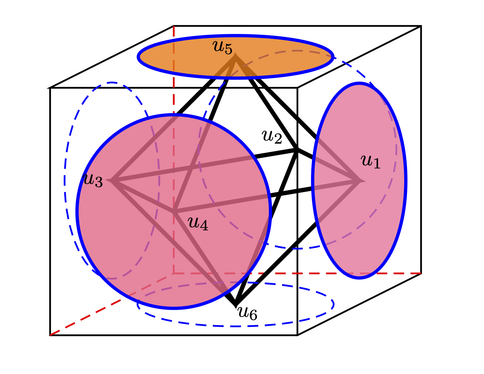
Of course, the single membrane model (42) is still too simplistic to model many physically integrated systems. A more realistic problem might instead involve a configuration of some number of coupled oscillating membranes. Consider, for example, a collection of six membranes arranged on corresponding faces of a cube, each coupled to its adjacent neighbors and modeled by a system of identical non-linear Helmholtz equations

(43) {Δu=f(α,z,u),uVu|D=0,\begin{cases}-\Delta u=f(\alpha,z,u),\quad u\in V\\ u|_{\partial D}=0,\end{cases}

where V=6V=\mathbb{R}^{6} and f:×D¯×VVf:\mathbb{R}\times\overline{D}\times V\rightarrow V is the vector-valued function

(44) f(α,z,u)=[f1(α,z,u1,u2,u3,u4,u5,u6)f2(α,z,u1,u2,u3,u4,u5,u6)f3(α,z,u1,u2,u3,u4,u5,u6)f4(α,z,u1,u2,u3,u4,u5,u6)f5(α,z,u1,u2,u3,u4,u5,u6)f6(α,z,u1,u2,u3,u4,u5,u6)],u=[u1u2u3u4u5u6].f(\alpha,z,u)=\left[\begin{array}[]{c}f_{1}(\alpha,z,u_{1},u_{2},u_{3},u_{4},u_{5},u_{6})\\ f_{2}(\alpha,z,u_{1},u_{2},u_{3},u_{4},u_{5},u_{6})\\ f_{3}(\alpha,z,u_{1},u_{2},u_{3},u_{4},u_{5},u_{6})\\ f_{4}(\alpha,z,u_{1},u_{2},u_{3},u_{4},u_{5},u_{6})\\ f_{5}(\alpha,z,u_{1},u_{2},u_{3},u_{4},u_{5},u_{6})\\ f_{6}(\alpha,z,u_{1},u_{2},u_{3},u_{4},u_{5},u_{6})\end{array}\right],\quad u=\left[\begin{array}[]{c}u_{1}\\ u_{2}\\ u_{3}\\ u_{4}\\ u_{5}\\ u_{6}\end{array}\right].

For compatibility with the results derived in previous sections, we assume that (44) satisfies the following conditions:

  1. (E1E_{1})

    For all α\alpha\in\mathbb{R}, zDz\in D, u=(u1,u2,u3,u4,u5,u6)T6u=(u_{1},u_{2},u_{3},u_{4},u_{5},u_{6})^{T}\in\mathbb{R}^{6} and τ𝑶\tau\in\bm{O}

    τf(α,z,u1,u2,u3,u4,u5,u6)=f(α,z,uτ(1),uτ(2),uτ(3),uτ(4),uτ(5),uτ(6));\displaystyle\tau f(\alpha,z,u_{1},u_{2},u_{3},u_{4},u_{5},u_{6})=f(\alpha,z,u_{\tau(1)},u_{\tau(2)},u_{\tau(3)},u_{\tau(4)},u_{\tau(5)},u_{\tau(6)});
  2. (E2E_{2})

    For all α\alpha\in\mathbb{R}, zDz\in D, u=(u1,u2,u3,u4,u5,u6)T6u=(u_{1},u_{2},u_{3},u_{4},u_{5},u_{6})^{T}\in\mathbb{R}^{6} and eiθO(2)e^{i\theta}\in O(2)

    f(α,eiθz,u1,u2,u3,u4,u5,u6)=f(α,z,u1,u2,u3,u4,u5,u6).\displaystyle f(\alpha,e^{i\theta}z,u_{1},u_{2},u_{3},u_{4},u_{5},u_{6})=f(\alpha,z,u_{1},u_{2},u_{3},u_{4},u_{5},u_{6}).
  3. (E3E_{3})

    For all α\alpha\in\mathbb{R}, zDz\in D, u=(u1,u2,u3,u4,u5,u6)T6u=(u_{1},u_{2},u_{3},u_{4},u_{5},u_{6})^{T}\in\mathbb{R}^{6},

    f(α,z,u1,u2,u3,u4,u5,u6)=f(α,z,u1,u2,u3,u4,u5,u6).\displaystyle f(\alpha,z,-u_{1},-u_{2},-u_{3},-u_{4},-u_{5},-u_{6})=-f(\alpha,z,u_{1},u_{2},u_{3},u_{4},u_{5},u_{6}).

Here, 𝑶S6\bm{O}\leq S_{6} is used to denote the chiral symmetry group of the cube, whose action on VV is described by the set of orientation preserving permutations of the corresponding membranes. If we identify S4S_{4} with 𝑶\bm{O} according to the rule

(1,2)(1,4)(2,3)(5,6),(1,2,3)(1,4,6)(3,5,2),\displaystyle(1,2)\;\;\;\leftrightarrow\;\;(1,4)(2,3)(5,6),\quad(1,2,3)\;\;\leftrightarrow\;\;(1,4,6)(3,5,2),
(1,2)(3,4)(1,4)(2,3),(1,2,3,4)(1,2,3,4),\displaystyle(1,2)(3,4)\;\;\leftrightarrow\;\;(1,4)(2,3),\quad(1,2,3,4)\;\;\leftrightarrow\;\;(1,2,3,4),

then the faces of the cube (see Figure 1) are naturally permuted as follows

(45) σ(u1,u2,u3,u4,u5,u6)T:=(uσ(1),uσ(2),uσ(3),uσ(4),uσ(5),uσ(6))T,σS4S6,uV.\displaystyle\sigma(u_{1},u_{2},u_{3},u_{4},u_{5},u_{6})^{T}:=(u_{\sigma(1)},u_{\sigma(2)},u_{\sigma(3)},u_{\sigma(4)},u_{\sigma(5)},u_{\sigma(6)})^{T},\quad\forall_{\sigma\in S_{4}\leq S_{6}},\;u\in V.

In this way, VV is an orthogonal S4S_{4}-representation with respect to the action (45). The table of characters for S4S_{4}

con. classes (1)(1) (1,2)(1,2) (1,2)(3,4)(1,2)(3,4) (1,2,3)(1,2,3) (1,2,3,4)(1,2,3,4)
χ0\chi_{0} 11 11 11 11 11
χ1\chi_{1} 11 1-1 11 11 1-1
χ2\chi_{2} 22 0 22 1-1 0
χ3\chi_{3} 33 1-1 1-1 0 11
χ4\chi_{4} 33 11 1-1 0 1-1
χV\chi_{V} 66 0 22 0 22
Table 1. Character Table for S4S_{4}.

reveals the relation

χV=χ0+χ2+χ3,\chi_{V}=\chi_{0}+\chi_{2}+\chi_{3},

which can be used to obtain the following S4×2S_{4}\times{\mathbb{Z}}_{2}-isotypic decomposition of VV

V=𝒱0𝒱2𝒱3.\displaystyle V=\mathcal{V}_{0}^{-}\oplus\mathcal{V}^{-}_{2}\oplus\mathcal{V}^{-}_{3}.

Under the assumptions (E1E_{1})-(E3E_{3}), the function ff clearly satisfies conditions (A1A_{1})-(A3A_{3}). Let us also assume that ff satisfies the conditions (A4A_{4}) and (A5A_{5}) with the matrix A(α):=Duf(0):VVA(\alpha):=D_{u}f(0):V\rightarrow V given by

(46) A(α)=aI+ζ(α)C,A(\alpha)=aI+\zeta(\alpha)C,

where I:VVI:V\rightarrow V is the identity matrix, C:VVC:V\rightarrow V is the weighted adjacency matrix

(47) C=[cd0ddddcd0dd0dcdddd0dcddddddc0dddd0c],C=\left[\begin{array}[c]{cccccc}c&d&0&d&d&d\\ d&c&d&0&d&d\\ 0&d&c&d&d&d\\ d&0&d&c&d&d\\ d&d&d&d&c&0\\ d&d&d&d&0&c\\ \end{array}\right],

defined for some fixed c,dc,d\in\mathbb{R} satisfying the conditions

  1. (E4E_{4})

    c>0c>0, d<0d<0, 4d+c04d+c\geq 0,

and where ζ:\zeta:\mathbb{R}\rightarrow\mathbb{R} is the sigmoid function

(48) ζ(α)=11+eα.\displaystyle\zeta(\alpha)=\frac{1}{1+e^{-\alpha}}.
α\alphaζ(α)=11+eα\zeta(\alpha)=\frac{1}{1+e^{-\alpha}}0.50.501.01.00
Figure 2. Graph of the sigmoid function ζ(α)\zeta(\alpha).
Remark 5.1.

The sigmoid function introduces a nonlinear dependence of the coupling in (43) on the bifurcation parameter α\alpha\in\mathbb{R}. Moreover, the asymptotic behaviour of (48) can be understood as the imposition of coupling strength saturation limits, which might reflect physical constraints such as, for example, bounded ranges for certain material densities.

With the linearization (46), system (43) clearly satisfies the condition (A~0\tilde{A}_{0}). Indeed, it can be shown that A(α):VVA(\alpha):V\rightarrow V admits three eigenvalues with eigenspaces corresponding to the S4S_{4}-isotypic components as follows

(49) μ0(α)\displaystyle\mu_{0}(\alpha) :=a+ζ(α)(c+4d),\displaystyle:=a+\zeta(\alpha)(c+4d), E(μ0(α))=𝒱0,\displaystyle E(\mu_{0}(\alpha))=\mathcal{V}_{0}^{-},
μ2(α)\displaystyle\mu_{2}(\alpha) :=a+ζ(α)(c2d),\displaystyle:=a+\zeta(\alpha)(c-2d), E(μ2(α))=𝒱2,\displaystyle E(\mu_{2}(\alpha))=\mathcal{V}_{2}^{-},
μ3(α)\displaystyle\mu_{3}(\alpha) :=a+ζ(α)c,\displaystyle:=a+\zeta(\alpha)c, E(μ3(α))=𝒱3.\displaystyle E(\mu_{3}(\alpha))=\mathcal{V}_{3}^{-}.

Notice also that, if c,dc,d\in\mathbb{R} are such that c+4d,c2d,c0c+4d,c-2d,c\neq 0, then the critical set associated with (44) is discrete. Together with the strict monotonicity of the eigenvalues (49) and the distinctness of the numbers snms_{nm}, it follows that each critical point of (43) can be specified by a unique triple (n,m,j)Σ(n,m,j)\in\Sigma with the notation

(50) αn,m,j:=μj1(snm).\displaystyle\alpha_{n,m,j}:=\mu_{j}^{-1}(s_{nm}).

We are now in a position to apply the local equivariant bifurcation results derived in this paper, namely Theorem 4.1 and Corollary 4.2, to the example system (43).

Proposition 5.1.

Under assumptions (E1E_{1})(E4E_{4}), every critical point αn,m,j\alpha_{n,m,j} of (43) is a branching point for a branch of non-trivial solutions with symmetries at least (Hs)({}^{s}H) for some orbit type of maximal kind (H)𝔐1,j(H)\in\mathfrak{M}_{1,j} and some folding sms\geq m.

Proof.

Let αn,m,j\alpha_{n,m,j} be a critical point of (43) with a deleted regular neighborhood αn,m,j<αn,m,j<αn,m,j+\alpha_{n,m,j}^{-}<\alpha_{n,m,j}<\alpha_{n,m,j}^{+} on which 𝒜(α)\mathscr{A}(\alpha) is an isomorphism and choose any orbit type of maximal kind (H)𝔐1,j(H)\in\mathfrak{M}_{1,j} with 2dim𝒱1,jH2\nmid\dim\mathcal{V}_{1,j}^{H}. The unique identification of (n,m,j)Σ(n,m,j)\in\Sigma with αn,m,j\alpha_{n,m,j} (cf. (50)) together with the strict monotonicity of the eigenvalues (49) imply the set difference Σ(αn,m,j+)Σ(αn,m,j)={(n,m,j)}\Sigma(\alpha_{n,m,j}^{+})\setminus\Sigma(\alpha_{n,m,j}^{-})=\{(n,m,j)\}. Therefore, the numbers 𝔫s(αn,m,j±,H)\mathfrak{n}^{s}(\alpha_{n,m,j}^{\pm},H) agree for all sms\neq m and are consecutive in the case of s=ms=m and the result follows from Corollary (4.2). \square In order to demonstrate how Theorem 4.3, the main global equivariant bifurcation result of this paper, can be applied to a system of the form (43), we introduce the following simplifying assumption:

  1. (E5E_{5})

    there exists an isotypic index j{0,2,3}j\in\{0,2,3\}, an odd number m021m_{0}\in 2{\mathbb{N}}-1 and a pair of numbers nl,nun_{l},n_{u}\in{\mathbb{N}} with nlnun_{l}\leq n_{u} and 2nunl2\mid n_{u}-n_{l} such that the Bessel root snms_{nm} lies:

    1. (i)

      within the codomain of μj\mu_{j} if m=m0m=m_{0} and nlnnun_{l}\leq n\leq n_{u};

    2. (ii)

      outside the codomain of μj\mu_{j} if either, m=m0m=m_{0} and n<nln<n_{l} or n>nun>n_{u}, or if m>m0m>m_{0} for any nn\in{\mathbb{N}}.

Condition (E5E_{5}) guarantees that an odd number of critical points (α,0)Λ𝑲(\alpha,0)\in\Lambda^{\bm{K}} will obtain 𝔰(α,H)=𝔰¯(H)\mathfrak{s}(\alpha,H)=\bar{\mathfrak{s}}(H) for every orbit type of maximal kind (H)𝔐1,j(H)\in\mathfrak{M}_{1,j} with 2dim𝒱1,jH2\nmid\dim\mathcal{V}_{1,j}^{H}.

Proposition 5.2.

Under assumptions (E1E_{1})(E5E_{5}), the trivial solution of (43) undergoes a global bifurcation of non-radial solutions with symmetries at least (Hs)({}^{s}H) at every critical point αn,m0,j\alpha_{n,m_{0},j} with nlnnun_{l}\leq n\leq n_{u} for every orbit type of maximal kind (H)𝔐1,j(H)\in\mathfrak{M}_{1,j} with 2dim𝒱1,jH2\nmid\dim\mathcal{V}_{1,j}^{H}.

Proof.

Choose (H)𝔐1,j(H)\in\mathfrak{M}_{1,j} with 2dim𝒱1,jH2\nmid\dim\mathcal{V}_{1,j}^{H} and notice that, since 𝔰¯(H)=m0\bar{\mathfrak{s}}(H)=m_{0} and αn,m0,j𝔍(H)\alpha_{n,m_{0},j}\in\mathfrak{J}(H) for every nlnnun_{l}\leq n\leq n_{u}, one has 2|𝔍(H)|2\nmid|\mathfrak{J}(H)| and the result follows from Theorem 4.3. \square So that Propositions 5.1 and 5.2 can be verified empirically, let us specify a particular bifurcation problem associated with system (43) by choosing the following values for the constants a,c,da,c,d\in\mathbb{R}

(51) a=32,c=5,d=1.\displaystyle a=32,\;c=5,\;d=-1.

For convenience, we include graphs of the three eigenvalues (49) with the assignments (51) in Figure 3 and the numbers snms_{nm} for m=0,,10m=0,\ldots,10 and n=1,,9n=1,\ldots,9 in Table 2.

n=1n=1 n=2n=2 n=3n=3 n=4n=4 n=5n=5 n=6n=6 n=7n=7 n=8n=8 n=9n=9
m=0 5.783 30.471 74.887 139.04 222.932 326.563 449.934 593.043 755.891
m=1 14.682 49.218 103.499 177.521 271.282 384.782 518.021 671 843.718
m=2 26.374 70.85 135.021 218.92 322.555 445.928 589.038 751.888 934.476
m=3 40.706 95.278 169.395 263.201 376.625 509.98 662.968 835.693 1028.15
m=4 57.583 122.428 206.57 310.322 433.761 576.913 739.79 922.398 1124.74
m=5 76.939 152.241 246.495 360.245 493.631 646.702 819.483 1011.99 1224.21
m=6 98.726 184.67 289.13 412.934 556.303 719.321 902.024 1104.44 1326.56
m=7 122.908 219.67 334.436 468.356 621.751 794.743 987.392 1199.73 1431.77
m=8 149.453 257.21 382.38 526.481 689.946 872.946 1075.56 1297.84 1539.81
m=9 178.337 297.26 432.933 587.281 760.863 953.907 1166.52 1398.77 1650.68
m=10 209.54 339.793 486.07 650.732 834.48 1037.6 1260.24 1502.48 1764.35
Table 2. Squared Zeros of Bessel functions snms_{nm} for 0m100\leq m\leq 10, 1n91\leq n\leq 9.
μ0(α)\mu_{0}(\alpha)μ2(α)\mu_{2}(\alpha)μ3(α)\mu_{3}(\alpha)s14=57.583s_{14}=57.583s13=40.706s_{13}=40.706s21=49.218s_{21}=49.218s20=30.471s_{20}=30.471
Figure 3. Graph of the eigenvalues μ0(α),μ2(α)\mu_{0}(\alpha),\mu_{2}(\alpha) and μ3(α)\mu_{3}(\alpha) and the consecutive numbers s20<s13<s21<s14s_{20}<s_{13}<s_{21}<s_{14}.

Notice that the critical set for (43) consists of exactly five critical points that can be distinguished, using the notation (50), as follows

(52) Λ={(α1,3,0,0),(α1,3,2,0),(α1,3,3,0),(α2,1,2,0),(α2,1,3,0)}.\displaystyle\Lambda=\{(\alpha_{1,3,0},0),(\alpha_{1,3,2},0),(\alpha_{1,3,3},0),(\alpha_{2,1,2},0),(\alpha_{2,1,3},0)\}.

In order to employ the results presented in previous sections to our bifurcation problem, we must first identify the maximal orbit types in Φ0(G;1{0})\Phi_{0}(G;\mathscr{H}_{1}\setminus\{0\}). The following G.A.P code can be used to generate a complete list of the sets 𝔐1,j\mathfrak{M}_{1,j} and the corresponding Basic Degrees deg𝒱1,j\deg_{\mathcal{V}_{1,j}} for j=1,2,3j=1,2,3.

1# A G.A.P Program for the computation of Maximal Orbit Types and Basic Degrees associated with the G-isotypic decomposition V = V_0 \times V_2 \times V_3
2LoadPackage ("EquiDeg");
3# create groups O(2)xS4xZ2
4o2:=OrthogonalGroupOverReal(2);
5s4:=SymmetricGroup(4);
6z2:=pCyclicGroup(2);
7# generate S4xZ2
8g1:=DirectProduct(s4,z2);
9# set names for subgroup conjugacy classes in S4xZ2
10SetCCSsAbbrv(g1, [ "Z1", "Z2", "D1z","D1","Z2m", "Z1p",
11"Z3", "V4", "D2z", "Z4", "D2", "D1p","D2d",
12"V4m", "D2p", "Z4d", "D3", "D3z", "Z3p",
13"V4p", "D4z", "D4d", "Z4p", "D4", "D4z",
14 "D4hd", "D3p", "A4", "D4p", "A4p", "S4", "S4m", "S4p"]);
15# generate O(2)xS4xZ2
16G:=DirectProduct(o2,g1);
17ccs:=ConjugacyClassesSubgroups(G);
18# find Maximal Orbit Types and Basic Degrees in first O(2)-isotypic component
19irrs := Irr(G);
20# The G-istoypic components 0,2,3 are indexed in G.A.P as 3,5,7
21for i in [ 3,5,7 ] do
22 max_orbtyps := MaximalOrbitTypes( irrs[1,i] );
23 basic_deg := BasicDegree( irrs[1,i] );
24 PrintFormatted( "\n Basic Degree associated with irrep V_{1,j} where j= \n", i );
25 View(basic_deg);
26 PrintFormatted( "\n Maximal Orbit Types in M_1,{} \n", i );
27 View(max_orbtyps);
28od;
29Print( "Done!\n" );

For any m>0m>0 and j{0,2,3}j\in\{0,2,3\}, the output of the above program can be used to describe the set of maximal orbit types 𝔐m,jΦ0(G)\mathfrak{M}_{m,j}\subset\Phi_{0}(G) the basic degrees deg𝒱m,jA(G)\deg_{\mathcal{V}_{m,j}}\in A(G) (cf. (25) and (26)), using amalgamated notation (cf. Appendix A), as follows:

𝔐m,0=\displaystyle\mathfrak{M}_{m,0}= {(D2mDm×S4S4p)},\displaystyle\Big{\{}(D_{2m}^{D_{m}}\times^{S_{4}}S_{4}^{p})\Big{\}},
𝔐m,2=\displaystyle\mathfrak{M}_{m,2}= {(D6mm×V4S4p),(D2mDm×D4D4p),(D2mDm×D4d^D4p)},\displaystyle\Big{\{}(D_{6m}^{{\mathbb{Z}}_{m}}\times^{V_{4}}S_{4}^{p}),(D_{2m}^{D_{m}}\times^{D_{4}}D_{4}^{p}),(D_{2m}^{D_{m}}\times^{D_{4}^{\hat{d}}}D_{4}^{p})\Big{\}},
𝔐m,3=\displaystyle\mathfrak{M}_{m,3}= {(D2mDm×D4zD4p),(D2mDm×D3zD3p),(D2mDm×D2dD4z),(D4mm×2D4p),(D6mm×D3p)},\displaystyle\Big{\{}(D_{2m}^{D_{m}}\times^{D_{4}^{z}}D_{4}^{p}),(D_{2m}^{D_{m}}\times^{D_{3}^{z}}D_{3}^{p}),(D_{2m}^{D_{m}}\times^{D_{2}^{d}}D_{4}^{z}),(D_{4m}^{{\mathbb{Z}}_{m}}\times^{{\mathbb{Z}}_{2}^{-}}D_{4}^{p}),(D_{6m}^{{\mathbb{Z}}_{m}}\times D_{3}^{p})\Big{\}},
deg𝒱m,0\displaystyle\deg_{\mathcal{V}_{m,0}} =(G)(D2mDm×S4S4p),\displaystyle=(G)-(D_{2m}^{D_{m}}\times^{S_{4}}S_{4}^{p}),
deg𝒱m,2\displaystyle\deg_{\mathcal{V}_{m,2}} =(G)2(D6mm×V4S4p)(D2mDm×D4D4p)(D2mDm×D4d^D4p)\displaystyle=(G)-2(D_{6m}^{{\mathbb{Z}}_{m}}\times^{V_{4}}S_{4}^{p})-(D_{2m}^{D_{m}}\times^{D_{4}}D_{4}^{p})-(D_{2m}^{D_{m}}\times^{D_{4}^{\hat{d}}}D_{4}^{p})
+(D2mDm×V4V4p)+4(D2mm×V4D4p),\displaystyle+(D_{2m}^{D_{m}}\times^{V_{4}}V_{4}^{p})+4(D_{2m}^{{\mathbb{Z}}_{m}}\times^{V_{4}}D_{4}^{p}),
deg𝒱m,3\displaystyle\deg_{\mathcal{V}_{m,3}} =(G)(D2mDm×D4zD4p)(D2mDm×D3zD3p)(D2mDm×D2dD4z)\displaystyle=(G)-(D_{2m}^{D_{m}}\times^{D_{4}^{z}}D_{4}^{p})-(D_{2m}^{D_{m}}\times^{D_{3}^{z}}D_{3}^{p})-(D_{2m}^{D_{m}}\times^{D_{2}^{d}}D_{4}^{z})
2(D4mm×2D4p)2(D6mm×D3p)+(D2mm×2D2p)\displaystyle-2(D_{4m}^{{\mathbb{Z}}_{m}}\times^{{\mathbb{Z}}_{2}^{-}}D_{4}^{p})-2(D_{6m}^{{\mathbb{Z}}_{m}}\times D_{3}^{p})+(D_{2m}^{{\mathbb{Z}}_{m}}\times^{{\mathbb{Z}}_{2}^{-}}D_{2}^{p})
+2(D2mm×2V4p)+2(D2mm×2D4z)+2(D2mm×D1zD4z)(D2mm×1p)2(D2mm×D2p).\displaystyle+2(D_{2m}^{{\mathbb{Z}}_{m}}\times^{{\mathbb{Z}}_{2}^{-}}V_{4}^{p})+2(D_{2m}^{{\mathbb{Z}}_{m}}\times^{{\mathbb{Z}}_{2}^{-}}D_{4}^{z})+2(D_{2m}^{{\mathbb{Z}}_{m}}\times^{D_{1}^{z}}D_{4}^{z})-(D_{2m}^{{\mathbb{Z}}_{m}}\times{\mathbb{Z}}_{1}^{p})-2(D_{2m}^{{\mathbb{Z}}_{m}}\times D_{2}^{p}).

We can deduce, from the coefficients of the Basic Degrees deg𝒱1,jA(G)\deg_{\mathcal{V}_{1,j}}\in A(G) (cf. Remark 4.3), that the fixed point space 𝒱1,jH\mathcal{V}_{1,j}^{H} has odd dimension for any j{0,2,3}j\in\{0,2,3\} and (H)𝔐1,j(H)\in\mathfrak{M}_{1,j}. Since the critical set (52) is manageably small, we also can manually compute the cardinalities (28) for each of the critical points (αn,m,j,0)Λ(\alpha_{n,m,j},0)\in\Lambda to obtain the quantities

{𝔰(α1,3,0,H)=3 if (H)𝔐1,0;𝔰(α1,3,2,H)=3,𝔰(α2,1,2,H)=1 if (H)𝔐1,2;𝔰(α1,3,3,H)=3,𝔰(α2,1,3,H)=1 if (H)𝔐1,3,\displaystyle\begin{cases}\mathfrak{s}(\alpha_{1,3,0},H)=3\quad&\text{ if }(H)\in\mathfrak{M}_{1,0};\\ \mathfrak{s}(\alpha_{1,3,2},H)=3,\;\mathfrak{s}(\alpha_{2,1,2},H)=1\quad&\text{ if }(H)\in\mathfrak{M}_{1,2};\\ \mathfrak{s}(\alpha_{1,3,3},H)=3,\;\mathfrak{s}(\alpha_{2,1,3},H)=1\quad&\text{ if }(H)\in\mathfrak{M}_{1,3},\end{cases}

and

{𝔦3(α1,3,0,H)=1 if (H)𝔐1,0;𝔦3(α1,3,2,H)=i1(α2,1,2,H)=1 if (H)𝔐1,2;𝔦3(α1,3,3,H)=i1(α2,1,3,H)=1 if (H)𝔐1,3.\displaystyle\begin{cases}\mathfrak{i}^{3}(\alpha_{1,3,0},H)=1\quad&\text{ if }(H)\in\mathfrak{M}_{1,0};\\ \mathfrak{i}^{3}(\alpha_{1,3,2},H)=i^{1}(\alpha_{2,1,2},H)=1\quad&\text{ if }(H)\in\mathfrak{M}_{1,2};\\ \mathfrak{i}^{3}(\alpha_{1,3,3},H)=i^{1}(\alpha_{2,1,3},H)=-1\quad&\text{ if }(H)\in\mathfrak{M}_{1,3}.\end{cases}

Therefore, from Theorem 4.1, it follows that every critical point (αn,m,j,0)Λ(\alpha_{n,m,j},0)\in\Lambda is a branching point for branches of non-trivial solutions to the problem (43) with symmetries at least (H3)({}^{3}H) in the case of (α1,3,2,0),(α1,3,3,0),(α1,3,0,0)Λ(\alpha_{1,3,2},0),(\alpha_{1,3,3},0),(\alpha_{1,3,0},0)\in\Lambda and with symmetries at least (H)(H) in the case of (α2,1,2,0),(α2,1,3,0)Λ(\alpha_{2,1,2},0),(\alpha_{2,1,3},0)\in\Lambda for each orbit type of maximal kind (H)𝔐1,j(H)\in\mathfrak{M}_{1,j}. The following G.A.P code can be used to computationally verify the non-triviality of the local bifurcation invariant (specifically, the non-triviality of the relevant coefficients) at each of the critical points in terms of the basic degrees

deg𝒱3,2,deg𝒱3,3,deg𝒱3,0,deg𝒱1,2,deg𝒱1,3A(G),\deg_{\mathcal{V}_{3,2}},\deg_{\mathcal{V}_{3,3}},\deg_{\mathcal{V}_{3,0}},\deg_{\mathcal{V}_{1,2}},\deg_{\mathcal{V}_{1,3}}\in A(G),

and the unit Burnside Ring element (G)(G) according to the rule derived in Lemma (4.2)

ωG(α1,3,2)\displaystyle\omega_{G}(\alpha_{1,3,2}) =(G)deg𝒱3,2,\displaystyle=(G)-\deg_{\mathcal{V}_{3,2}},
ωG(α1,3,3)\displaystyle\omega_{G}(\alpha_{1,3,3}) =deg𝒱3,2deg𝒱3,2deg𝒱3,3,\displaystyle=\deg_{\mathcal{V}_{3,2}}-\deg_{\mathcal{V}_{3,2}}\cdot\deg_{\mathcal{V}_{3,3}},
ωG(α1,3,0)\displaystyle\omega_{G}(\alpha_{1,3,0}) =deg𝒱3,2deg𝒱3,3deg𝒱3,2deg𝒱3,3deg𝒱3,0,\displaystyle=\deg_{\mathcal{V}_{3,2}}\cdot\deg_{\mathcal{V}_{3,3}}-\deg_{\mathcal{V}_{3,2}}\cdot\deg_{\mathcal{V}_{3,3}}\cdot\deg_{\mathcal{V}_{3,0}},
ωG(α2,1,2)\displaystyle\omega_{G}(\alpha_{2,1,2}) =deg𝒱3,2deg𝒱3,3deg𝒱3,0deg𝒱3,2deg𝒱3,3deg𝒱3,0deg𝒱1,2,\displaystyle=\deg_{\mathcal{V}_{3,2}}\cdot\deg_{\mathcal{V}_{3,3}}\cdot\deg_{\mathcal{V}_{3,0}}-\deg_{\mathcal{V}_{3,2}}\cdot\deg_{\mathcal{V}_{3,3}}\cdot\deg_{\mathcal{V}_{3,0}}\cdot\deg_{\mathcal{V}_{1,2}},
ωG(α2,1,3)\displaystyle\omega_{G}(\alpha_{2,1,3}) =deg𝒱3,2deg𝒱3,3deg𝒱3,0deg𝒱1,2deg𝒱3,2deg𝒱3,3deg𝒱3,0deg𝒱1,2deg𝒱1,3.\displaystyle=\deg_{\mathcal{V}_{3,2}}\cdot\deg_{\mathcal{V}_{3,3}}\cdot\deg_{\mathcal{V}_{3,0}}\cdot\deg_{\mathcal{V}_{1,2}}-\deg_{\mathcal{V}_{3,2}}\cdot\deg_{\mathcal{V}_{3,3}}\cdot\deg_{\mathcal{V}_{3,0}}\cdot\deg_{\mathcal{V}_{1,2}}\cdot\deg_{\mathcal{V}_{1,3}}.
1# A G.A.P Program for the Burnside Ring product of Basic Degrees to be used for the verification of non-triviality of local bifurcation invariants
2# Initialize the Burnside Ring A(G), with unit element U =(G)
3AG:=BurnsideRing(G); H:=Basis(AG); U:=H[0,131];
4# Initialize the relevant Basic Degrees
5d_30 := BasicDegree(Irr(G)[3,3]);
6d_32 := BasicDegree(Irr(G)[3,5]);
7d_33 := BasicDegree(Irr(G)[3,7]);
8d_12 := BasicDegree(Irr(G)[1,5]);
9d_13 := BasicDegree(Irr(G)[1,7]);
10# Compute Products of Basic Degrees Cumulatively
11p_1 := d_32; p_2 := p_1*d_33; p_3 := p_2*d_30;
12p_4 := p_3*d_12; p_5 := p_4*d_13;
13# Compute the local bifurcation invariants w_{n,m,j}
14w_132 := U - p_1; w_133 := p_1 - p_2; w_130 := p_2 - p_3;
15w_212 := p_3 - p_4; w_213 := p_4 - p_5;
16# Sum the local bifurcation invariants
17sum := w_132 + w_133 + w_130 + w_212 + w_213

The output of the above program can be expressed using amalgamated notation as follows:

ωG(α1,3,2)\displaystyle\omega_{G}(\alpha_{1,3,2}) =4(D63×V4D4p)(D6D3×V4V4p)+(D6D3×D4D4p)+(D6D3×D4d^D4p)\displaystyle=-4(D_{6}^{{\mathbb{Z}}_{3}}\times^{V_{4}}D_{4}^{p})-(D_{6}^{D_{3}}\times^{V_{4}}V_{4}^{p})+(D_{6}^{D_{3}}\times^{D_{4}}D_{4}^{p})+(D_{6}^{D_{3}}\times^{D_{4}^{\hat{d}}}D_{4}^{p})
+2(D183×V4S4p),\displaystyle\quad+2(D_{18}^{{\mathbb{Z}}_{3}}\times^{V_{4}}S_{4}^{p}),
ωG(α1,3,3)\displaystyle\omega_{G}(\alpha_{1,3,3}) =4(D63×1D1p)+2(D63×1D2p)+(D6D3×11p)2(D63×D1D4z)\displaystyle=4(D_{6}^{{\mathbb{Z}}_{3}}\times^{{\mathbb{Z}}_{1}}D_{1}^{p})+2(D_{6}^{{\mathbb{Z}}_{3}}\times^{{\mathbb{Z}}_{1}}D_{2}^{p})+(D_{6}^{D_{3}}\times^{{\mathbb{Z}}_{1}}{\mathbb{Z}}_{1}^{p})-2(D_{6}^{{\mathbb{Z}}_{3}}\times^{D_{1}}D_{4}^{z})
2(D63×2D4z)2(D63×2V4p)+2(D63×24p)+2(D63×2D4z)\displaystyle\quad-2(D_{6}^{{\mathbb{Z}}_{3}}\times^{{\mathbb{Z}}_{2}^{-}}D_{4}^{z})-2(D_{6}^{{\mathbb{Z}}_{3}}\times^{{\mathbb{Z}}_{2}^{-}}V_{4}^{p})+2(D_{6}^{{\mathbb{Z}}_{3}}\times^{{\mathbb{Z}}_{2}}{\mathbb{Z}}_{4}^{p})+2(D_{6}^{{\mathbb{Z}}_{3}}\times^{{\mathbb{Z}}_{2}}D_{4}^{z})
+2(D63×2V4p)(D6D3×D1D1p)(D6D3×D1zD1p)(D6D3×2D2p)\displaystyle\quad+2(D_{6}^{{\mathbb{Z}}_{3}}\times^{{\mathbb{Z}}_{2}}V_{4}^{p})-(D_{6}^{D_{3}}\times^{D_{1}}D_{1}^{p})-(D_{6}^{D_{3}}\times^{D_{1}^{z}}D_{1}^{p})-(D_{6}^{D_{3}}\times^{{\mathbb{Z}}_{2}^{-}}D_{2}^{p})
+(D6D3×2D2p)2(D183×1D3p)+2(D123×2D4p)2(D63×4D4p)\displaystyle\quad+(D_{6}^{D_{3}}\times^{{\mathbb{Z}}_{2}}D_{2}^{p})-2(D_{18}^{{\mathbb{Z}}_{3}}\times^{{\mathbb{Z}}_{1}}D_{3}^{p})+2(D_{12}^{{\mathbb{Z}}_{3}}\times^{{\mathbb{Z}}_{2}^{-}}D_{4}^{p})-2(D_{6}^{{\mathbb{Z}}_{3}}\times^{{\mathbb{Z}}_{4}}D_{4}^{p})
2(D63×D2zD4p)+(D6D3×D2dD4z)(D6D3×44p)(D6D3×D2zD4z)\displaystyle\quad-2(D_{6}^{{\mathbb{Z}}_{3}}\times^{D_{2}^{z}}D_{4}^{p})+(D_{6}^{D_{3}}\times^{D_{2}^{d}}D_{4}^{z})-(D_{6}^{D_{3}}\times^{{\mathbb{Z}}_{4}}{\mathbb{Z}}_{4}^{p})-(D_{6}^{D_{3}}\times^{D_{2}^{z}}D_{4}^{z})
+(D6D3×D3zD3p)+(D6D3×D4zD4p),\displaystyle\quad+(D_{6}^{D_{3}}\times^{D_{3}^{z}}D_{3}^{p})+(D_{6}^{D_{3}}\times^{D_{4}^{z}}D_{4}^{p}),
ωG(α1,3,0)\displaystyle\omega_{G}(\alpha_{1,3,0}) =2(D63×D1D4z)2(D63×24p)2(D63×2D4z)2(D63×2V4p)\displaystyle=2(D_{6}^{{\mathbb{Z}}_{3}}\times^{D_{1}}D_{4}^{z})-2(D_{6}^{{\mathbb{Z}}_{3}}\times^{{\mathbb{Z}}_{2}}{\mathbb{Z}}_{4}^{p})-2(D_{6}^{{\mathbb{Z}}_{3}}\times^{{\mathbb{Z}}_{2}}D_{4}^{z})-2(D_{6}^{{\mathbb{Z}}_{3}}\times^{{\mathbb{Z}}_{2}}V_{4}^{p})
+(D6D3×D1D1p)(D6D3×2D2p)2(D63×3D3p)(D6D3×33p)\displaystyle\quad+(D_{6}^{D_{3}}\times^{D_{1}}D_{1}^{p})-(D_{6}^{D_{3}}\times^{{\mathbb{Z}}_{2}}D_{2}^{p})-2(D_{6}^{{\mathbb{Z}}_{3}}\times^{{\mathbb{Z}}_{3}}D_{3}^{p})-(D_{6}^{D_{3}}\times^{{\mathbb{Z}}_{3}}{\mathbb{Z}}_{3}^{p})
+2(D63×4D4p)+3(D63×V4D4p)+(D6D3×44p)+(D6D3×V4V4p)\displaystyle\quad+2(D_{6}^{{\mathbb{Z}}_{3}}\times^{{\mathbb{Z}}_{4}}D_{4}^{p})+3(D_{6}^{{\mathbb{Z}}_{3}}\times^{V_{4}}D_{4}^{p})+(D_{6}^{D_{3}}\times^{{\mathbb{Z}}_{4}}{\mathbb{Z}}_{4}^{p})+(D_{6}^{D_{3}}\times^{V_{4}}V_{4}^{p})
2(D6D3×D4D4p)+(D6D3×S4S4p)\displaystyle\quad-2(D_{6}^{D_{3}}\times^{D_{4}}D_{4}^{p})+(D_{6}^{D_{3}}\times^{S_{4}}S_{4}^{p})
ωG(α2,1,2)\displaystyle\omega_{G}(\alpha_{2,1,2}) =2(D21×1D2p)+(D2D1×11p)2(D21×D1D4z)2(D21×D1zD4z)\displaystyle=2(D_{2}^{{\mathbb{Z}}_{1}}\times^{{\mathbb{Z}}_{1}}D_{2}^{p})+(D_{2}^{D_{1}}\times^{{\mathbb{Z}}_{1}}{\mathbb{Z}}_{1}^{p})-2(D_{2}^{{\mathbb{Z}}_{1}}\times^{D_{1}}D_{4}^{z})-2(D_{2}^{{\mathbb{Z}}_{1}}\times^{D_{1}^{z}}D_{4}^{z})
(D2D1×D1D1p)(D2D1×D1zD1p)+4(D61×1D3p)2(D21×4D4p)\displaystyle\quad-(D_{2}^{D_{1}}\times^{D_{1}}D_{1}^{p})-(D_{2}^{D_{1}}\times^{D_{1}^{z}}D_{1}^{p})+4(D_{6}^{{\mathbb{Z}}_{1}}\times^{{\mathbb{Z}}_{1}}D_{3}^{p})-2(D_{2}^{{\mathbb{Z}}_{1}}\times^{{\mathbb{Z}}_{4}}D_{4}^{p})
+2(D21×D2zD4p)+2(D21×V4D4p)(D2D1×44p)+(D2D1×D2zD4z)\displaystyle\quad+2(D_{2}^{{\mathbb{Z}}_{1}}\times^{D_{2}^{z}}D_{4}^{p})+2(D_{2}^{{\mathbb{Z}}_{1}}\times^{V_{4}}D_{4}^{p})-(D_{2}^{D_{1}}\times^{{\mathbb{Z}}_{4}}{\mathbb{Z}}_{4}^{p})+(D_{2}^{D_{1}}\times^{D_{2}^{z}}D_{4}^{z})
+(D2D1×D4D4p)(D2D1×D4d^D4p)2(D61×V4S4p)\displaystyle\quad+(D_{2}^{D_{1}}\times^{D_{4}}D_{4}^{p})-(D_{2}^{D_{1}}\times^{D_{4}^{\hat{d}}}D_{4}^{p})-2(D_{6}^{{\mathbb{Z}}_{1}}\times^{V_{4}}S_{4}^{p})
ωG(α2,1,3)\displaystyle\omega_{G}(\alpha_{2,1,3}) =4(D21×1D1p)4(D21×1D2p)2(D2D1×11p)+2(D21×D1D4z)\displaystyle=-4(D_{2}^{{\mathbb{Z}}_{1}}\times^{{\mathbb{Z}}_{1}}D_{1}^{p})-4(D_{2}^{{\mathbb{Z}}_{1}}\times^{{\mathbb{Z}}_{1}}D_{2}^{p})-2(D_{2}^{D_{1}}\times^{{\mathbb{Z}}_{1}}{\mathbb{Z}}_{1}^{p})+2(D_{2}^{{\mathbb{Z}}_{1}}\times^{D_{1}}D_{4}^{z})
+2(D21×D1zD4z)+2(D21×2D4z)+2(D21×2V4p)+(D2D1×D1D1p)\displaystyle\quad+2(D_{2}^{{\mathbb{Z}}_{1}}\times^{D_{1}^{z}}D_{4}^{z})+2(D_{2}^{{\mathbb{Z}}_{1}}\times^{{\mathbb{Z}}_{2}^{-}}D_{4}^{z})+2(D_{2}^{{\mathbb{Z}}_{1}}\times^{{\mathbb{Z}}_{2}^{-}}V_{4}^{p})+(D_{2}^{D_{1}}\times^{D_{1}}D_{1}^{p})
+2(D2D1×D1zD1p)+(D2D1×2D2p)2(D61×1D3p)+2(D21×3D3p)\displaystyle\quad+2(D_{2}^{D_{1}}\times^{D_{1}^{z}}D_{1}^{p})+(D_{2}^{D_{1}}\times^{{\mathbb{Z}}_{2}^{-}}D_{2}^{p})-2(D_{6}^{{\mathbb{Z}}_{1}}\times^{{\mathbb{Z}}_{1}}D_{3}^{p})+2(D_{2}^{{\mathbb{Z}}_{1}}\times^{{\mathbb{Z}}_{3}}D_{3}^{p})
+(D2D1×33p)2(D41×2D4p)+2(D21×4D4p)(D2D1×D2dD4z)\displaystyle\quad+(D_{2}^{D_{1}}\times^{{\mathbb{Z}}_{3}}{\mathbb{Z}}_{3}^{p})-2(D_{4}^{{\mathbb{Z}}_{1}}\times^{{\mathbb{Z}}_{2}^{-}}D_{4}^{p})+2(D_{2}^{{\mathbb{Z}}_{1}}\times^{{\mathbb{Z}}_{4}}D_{4}^{p})-(D_{2}^{D_{1}}\times^{D_{2}^{d}}D_{4}^{z})
+(D2D1×44p)+(D2D1×D3zD3p)(D2D1×D4zD4p).\displaystyle\quad+(D_{2}^{D_{1}}\times^{{\mathbb{Z}}_{4}}{\mathbb{Z}}_{4}^{p})+(D_{2}^{D_{1}}\times^{D_{3}^{z}}D_{3}^{p})-(D_{2}^{D_{1}}\times^{D_{4}^{z}}D_{4}^{p}).

Next, we can determine the global behaviour of some of the branches predicted using Theorem (4.1) by establishing the parity of the set (40). Notice that, for every j{0,2,3}j\in\{0,2,3\} and (H)𝔐1,j(H)\in\mathfrak{M}_{1,j}, the quantity 𝔰¯(H)=3\bar{\mathfrak{s}}(H)=3 is obtained for exactly one critical point (α1,3,j,0)(\alpha_{1,3,j},0), i.e.

𝔍(H)={{(α1,3,0,0)} if (H)𝔐1,0;{(α1,3,2,0)} if (H)𝔐1,2;{(α1,3,3,0)} if (H)𝔐1,3.\displaystyle\mathfrak{J}(H)=\begin{cases}\{(\alpha_{1,3,0},0)\}\quad&\text{ if }(H)\in\mathfrak{M}_{1,0};\\ \{(\alpha_{1,3,2},0)\}\quad&\text{ if }(H)\in\mathfrak{M}_{1,2};\\ \{(\alpha_{1,3,3},0)\}\quad&\text{ if }(H)\in\mathfrak{M}_{1,3}.\end{cases}

Therefore, any branch of non-trivial solutions with symmetries at least (H3)({}^{3}H) bifurcating from (α1,3,j,0)(\alpha_{1,3,j},0), for every j{0,2,3}j\in\{0,2,3\} and (H)𝔐1,j(H)\in\mathfrak{M}_{1,j}, consists only of non-radial solutions and is unbounded. Of course, since the critical set (52) is finite, one needs only sum the relevant local bifurcation invariants to arrive at the same conclusion directly from the Rabinowitz alternative (cf. Theorems 4.2 and 4.3).

(α0,0)ΛωG(α0)\displaystyle\sum_{(\alpha_{0},0)\in\Lambda}\omega_{G}(\alpha_{0}) =ωG(α1,3,2)+ωG(α1,3,3)+ωG(α1,3,0)+ωG(α2,1,2)+ωG(α2,1,3)\displaystyle=\omega_{G}(\alpha_{1,3,2})+\omega_{G}(\alpha_{1,3,3})+\omega_{G}(\alpha_{1,3,0})+\omega_{G}(\alpha_{2,1,2})+\omega_{G}(\alpha_{2,1,3})
=4(D21×1D1p)2(D21×1D2p)(D2D1×11p)+2(D21×2D4z)\displaystyle=-4(D_{2}^{{\mathbb{Z}}_{1}}\times^{{\mathbb{Z}}_{1}}D_{1}^{p})-2(D_{2}^{{\mathbb{Z}}_{1}}\times^{{\mathbb{Z}}_{1}}D_{2}^{p})-(D_{2}^{D_{1}}\times^{{\mathbb{Z}}_{1}}{\mathbb{Z}}_{1}^{p})+2(D_{2}^{{\mathbb{Z}}_{1}}\times^{{\mathbb{Z}}_{2}^{-}}D_{4}^{z})
+2(D21×2V4p)+(D2D1×D1zD1p)+(D2D1×2D2p)+2(D61×1D3p)\displaystyle\quad+2(D_{2}^{{\mathbb{Z}}_{1}}\times^{{\mathbb{Z}}_{2}^{-}}V_{4}^{p})+(D_{2}^{D_{1}}\times^{D_{1}^{z}}D_{1}^{p})+(D_{2}^{D_{1}}\times^{{\mathbb{Z}}_{2}^{-}}D_{2}^{p})+2(D_{6}^{{\mathbb{Z}}_{1}}\times^{{\mathbb{Z}}_{1}}D_{3}^{p})
+2(D21×3D3p)+(D2D1×33p)2(D41×2D4p)+2(D21×D2zD4p)\displaystyle\quad+2(D_{2}^{{\mathbb{Z}}_{1}}\times^{{\mathbb{Z}}_{3}}D_{3}^{p})+(D_{2}^{D_{1}}\times^{{\mathbb{Z}}_{3}}{\mathbb{Z}}_{3}^{p})-2(D_{4}^{{\mathbb{Z}}_{1}}\times^{{\mathbb{Z}}_{2}^{-}}D_{4}^{p})+2(D_{2}^{{\mathbb{Z}}_{1}}\times^{D_{2}^{z}}D_{4}^{p})
+2(D21×V4D4p)(D2D1×D2dD4z)+(D2D1×D2zD4z)(D2D1×D3zD3p)\displaystyle\quad+2(D_{2}^{{\mathbb{Z}}_{1}}\times^{V_{4}}D_{4}^{p})-(D_{2}^{D_{1}}\times^{D_{2}^{d}}D_{4}^{z})+(D_{2}^{D_{1}}\times^{D_{2}^{z}}D_{4}^{z})-(D_{2}^{D_{1}}\times^{D_{3}^{z}}D_{3}^{p})
(D2D1×D4zD4p)+(D2D1×D4D4p)(D2D1×D4d^D4p)2(D61×V4S4p)\displaystyle\quad-(D_{2}^{D_{1}}\times^{D_{4}^{z}}D_{4}^{p})+(D_{2}^{D_{1}}\times^{D_{4}}D_{4}^{p})-(D_{2}^{D_{1}}\times^{D_{4}^{\hat{d}}}D_{4}^{p})-2(D_{6}^{{\mathbb{Z}}_{1}}\times^{V_{4}}S_{4}^{p})
+4(D63×1D1p)+2(D63×1D2p)+(D6D3×11p)2(D63×2D4z)\displaystyle\quad+4(D_{6}^{{\mathbb{Z}}_{3}}\times^{{\mathbb{Z}}_{1}}D_{1}^{p})+2(D_{6}^{{\mathbb{Z}}_{3}}\times^{{\mathbb{Z}}_{1}}D_{2}^{p})+(D_{6}^{D_{3}}\times^{{\mathbb{Z}}_{1}}{\mathbb{Z}}_{1}^{p})-2(D_{6}^{{\mathbb{Z}}_{3}}\times^{{\mathbb{Z}}_{2}^{-}}D_{4}^{z})
2(D63×2V4p)(D6D3×D1zD1p)(D6D3×2D2p)2(D183×1D3p)\displaystyle\quad-2(D_{6}^{{\mathbb{Z}}_{3}}\times^{{\mathbb{Z}}_{2}^{-}}V_{4}^{p})-(D_{6}^{D_{3}}\times^{D_{1}^{z}}D_{1}^{p})-(D_{6}^{D_{3}}\times^{{\mathbb{Z}}_{2}^{-}}D_{2}^{p})-2(D_{1}8^{{\mathbb{Z}}_{3}}\times^{{\mathbb{Z}}_{1}}D_{3}^{p})
2(D63×3D3p)(D6D3×33p)+2(D123×2D4p)2(D63×D2zD4p)\displaystyle\quad-2(D_{6}^{{\mathbb{Z}}_{3}}\times^{{\mathbb{Z}}_{3}}D_{3}^{p})-(D_{6}^{D_{3}}\times^{{\mathbb{Z}}_{3}}{\mathbb{Z}}_{3}^{p})+2(D_{1}2^{{\mathbb{Z}}_{3}}\times^{{\mathbb{Z}}_{2}^{-}}D_{4}^{p})-2(D_{6}^{{\mathbb{Z}}_{3}}\times^{D_{2}^{z}}D_{4}^{p})
2(D63×V4D4p)+(D6D3×D2dD4z)(D6D3×D2zD4z)+(D6D3×D3zD3p)\displaystyle\quad-2(D_{6}^{{\mathbb{Z}}_{3}}\times^{V_{4}}D_{4}^{p})+(D_{6}^{D_{3}}\times^{D_{2}^{d}}D_{4}^{z})-(D_{6}^{D_{3}}\times^{D_{2}^{z}}D_{4}^{z})+(D_{6}^{D_{3}}\times^{D_{3}^{z}}D_{3}^{p})
+(D6D3×D4zD4p)(D6D3×D4D4p)+(D6D3×D4d^D4p)+2(D183×V4S4p)\displaystyle\quad+(D_{6}^{D_{3}}\times^{D_{4}^{z}}D_{4}^{p})-(D_{6}^{D_{3}}\times^{D_{4}}D_{4}^{p})+(D_{6}^{D_{3}}\times^{D_{4}^{\hat{d}}}D_{4}^{p})+2(D_{18}^{{\mathbb{Z}}_{3}}\times^{V_{4}}S_{4}^{p})
+(D6D3×S4S4p).\displaystyle\quad+(D_{6}^{D_{3}}\times^{S_{4}}S_{4}^{p}).

In closing, let’s consider a closer interpretation of the above results. Take the maximal orbit type (H)=(D2D1×D4D4p)𝔐1,2(H)=(D_{2}^{D_{1}}\times^{D_{4}}D_{4}^{p})\in\mathfrak{M}_{1,2} and let 𝒞\mathcal{C} be a branch of non-radial solutions with symmetries at least (H3)=(D6D3×D4D4p)𝔐3,2({}^{3}H)=(D_{6}^{D_{3}}\times^{D_{4}}D_{4}^{p})\in\mathfrak{M}_{3,2} emerging from the first critical point (α1,3,2,0)Λ(\alpha_{1,3,2},0)\in\Lambda. Notice that the kernel of 𝒜(α):\mathscr{A}(\alpha):\mathscr{H}\rightarrow\mathscr{H} at any critical point (αn,m,j,0)Λ(\alpha_{n,m,j},0)\in\Lambda is given by the corresponding irreducible GG-representation n,mj\mathscr{E}_{n,m}^{j} (cf. (16)), i.e.

Ker 𝒜(α1,3,2)=1,32\text{\rm Ker\,}\mathscr{A}(\alpha_{1,3,2})=\mathscr{E}_{1,3}^{2}

such that any vector u^\hat{u}\in\mathscr{H} with 𝒜(α1,3,2)u^=0\mathscr{A}(\alpha_{1,3,2})\hat{u}=0 must be of the form

u^(r,θ){J3(s13r)(cos(3θ)a+sin(3θ)b):a,bspan{w1,w2}},\hat{u}(r,\theta)\in\left\{J_{3}(\sqrt{s_{13}}r)\Big{(}\cos(3\theta)\vec{a}+\sin(3\theta)\vec{b}\Big{)}:\vec{a},\,\vec{b}\in\text{span}\{\vec{w}_{1},\vec{w}_{2}\}\right\},

where w1,w2𝒱2\vec{w}_{1},\vec{w}_{2}\in\mathcal{V}_{2}^{-} are the eigenvectors

w1=(1,1,1,1,0,0)T and w2=(1,0,1,0,1,1)T.\vec{w}_{1}=(-1,1,-1,1,0,0)^{T}\text{ and }\vec{w}_{2}=(1,0,1,0,-1,-1)^{T}.

Computing the generators of the orbit type (D6D3×D4D4p)(D_{6}^{D_{3}}\times^{D_{4}}D_{4}^{p}),

(2π3,(1),1),(κ,(1),1),(eSO(2),(1,2,3,4),1),(eSO(2),(1,2),1),(π3,(1),1)H\displaystyle\left(\frac{2\pi}{3},(1),1\right),\;\left(\kappa,(1),1\right),\;\left(e_{SO(2)},(1,2,3,4),1\right),\;\left(e_{SO(2)},(1,2),1\right),\;\left(\frac{\pi}{3},(1),-1\right)\in H

and examining their action (cf. (14), (45)) on 1,32\mathscr{E}_{1,3}^{2}, we observe the radial invariances

u^(r,θ+2π3)=u^(r,θ) andu^(r,θ+π3)=u^(r,θ),\hat{u}(r,\theta+\frac{2\pi}{3})=\hat{u}(r,\theta)\text{ and}-\hat{u}(r,\theta+\frac{\pi}{3})=\hat{u}(r,\theta),

which are satisfied trivially for all elements of 1,23\mathscr{E}_{1,2}^{3}, the conjugate invariance

u^(r,θ)=u^(r,θ),\hat{u}(r,-\theta)=\hat{u}(r,\theta),

which is only satisfied when b=0\vec{b}=\vec{0}, and also the permutation invariances

(1,2,3,4)u^(r,θ)=u^(r,θ) and (1,2)u^(r,θ)=u^(r,θ),(1,2,3,4)\cdot\hat{u}(r,\theta)=\hat{u}(r,\theta)\text{ and }(1,2)\cdot\hat{u}(r,\theta)=\hat{u}(r,\theta),

which, for a=a1w1+a2w2\vec{a}=a_{1}\vec{w}_{1}+a_{2}\vec{w}_{2}, is satisfied if and only if a2=2a1a_{2}=2a_{1}. Moreover, since one has dimKer 𝒜(α0)H=1\dim\text{\rm Ker\,}\mathscr{A}(\alpha_{0})^{H}=1, the celebrated theorem of Crandall-Rabinowitz (cf. [29]) guarantees that the branch 𝒞\mathcal{C} is tangent to the solution u^(r,θ)=J3(s13r)cos(3θ)(w1+2w2)\hat{u}(r,\theta)=J_{3}(\sqrt{s_{13}}r)\cos(3\theta)(\vec{w}_{1}+2\vec{w}_{2}) at the point (α1,3,2,0)(\alpha_{1,3,2},0). Therefore, u^\hat{u}\in\mathscr{H} can reasonably be used to estimate the behaviour of the branch 𝒞\mathcal{C} for parameter values near α1,3,2\alpha_{1,3,2}\in\mathbb{R}.

Refer to caption
Figure 4. Graph of the map u^(r,θ)=J3(s13r)cos(3θ)(w1+2w2)\hat{u}(r,\theta)=J_{3}(\sqrt{s_{13}}r)\cos(3\theta)(\vec{w}_{1}+2\vec{w}_{2}).

Appendix A Amalgamated Notation of Subgroups

The convention of amalgamated notation is a shorthand for the specification of subgroups and their conjugacy classes in a product group G1×G2G_{1}\times G_{2}. In order to introduce this convention, we recall a well-known consequence of Goursat’s Lemma (cf. [15]). Namely that, for any closed subgroup in HG1×G2H\leq G_{1}\times G_{2}, there are two subgroups K1G1K_{1}\leq G_{1}, K2G2K_{2}\leq G_{2}, a group LL and a pair of epimorphisms φ2:K1L\varphi_{2}:K_{1}\rightarrow L, φ2:K2L\varphi_{2}:K_{2}\rightarrow L such that

(53) H={(x,y)K1×K2:φ1(x)=φ2(y)}.\displaystyle H=\{(x,y)\in K_{1}\times K_{2}\;:\;\varphi_{1}(x)=\varphi_{2}(y)\}.

Using amalgamated notation, the subgroup (53) is identified, up to its conjugacy class in Φ0(G1×G2)\Phi_{0}(G_{1}\times G_{2}), by the quintuple (K1,K2,L,Z1,Z2)(K_{1},K_{2},L,Z_{1},Z_{2}), where Z1:=Ker φ1Z_{1}:=\text{\rm Ker\,}\varphi_{1} and Z2:=Ker φ2Z_{2}:=\text{\rm Ker\,}\varphi_{2}, as follows

(H)=(K1×LZ2Z1K2).\displaystyle(H)=(K_{1}{}^{Z_{1}}\times^{Z_{2}}_{L}K_{2}).

In particular, one can always choose the group LL such that LK1/Z1L\simeq K_{1}/Z_{1}, in which case the conjugacy class of (53) is identified with the quadruple (K1,K1,Z1,Z2)(K_{1},K_{1},Z_{1},Z_{2}) as follows

(54) (H)=(K1×Z2Z1K2).\displaystyle(H)=(K_{1}{}^{Z_{1}}\times^{Z_{2}}K_{2}).

This compact amalgamated decomposition (54) is the form with which subgroup conjugacy classes are identified in this paper. In addition to the notation defined above, the following list provides some ancillary shorthand used in this paper for the identification of subgroups in S4×2S_{4}\times{\mathbb{Z}}_{2}

2\displaystyle{\mathbb{Z}}_{2}^{-} ={((1),1),((12)(34),1)},\displaystyle=\{((1),1),((12)(34),-1)\},
4\displaystyle{\mathbb{Z}}_{4}^{-} ={((1),1),((1324),1),((12)(34),1),((1423),1)},\displaystyle=\{((1),1),((1324),-1),((12)(34),1),((1423),-1)\},
D1z\displaystyle D_{1}^{z} ={((1),1),((12),1)},\displaystyle=\{((1),1),((12),-1)\},
V4\displaystyle V_{4}^{-} ={((1),1),((12)(34),1),((13)(24),1),((14)(23),1)},\displaystyle=\{((1),1),((12)(34),1),((13)(24),-1),((14)(23),-1)\},
D2d\displaystyle D_{2}^{d} ={((1),1),((12)(34),1),((12),1),((34),1)},\displaystyle=\{((1),1),((12)(34),-1),((12),1),((34),-1)\},
D2z\displaystyle D_{2}^{z} ={((1),1),((12)(34),1),((12),1),((34),1)},\displaystyle=\{((1),1),((12)(34),1),((12),-1),((34),-1)\},
D3z\displaystyle D_{3}^{z} ={((1),1),((123),1),((132),1),((12),1),((23),1),((13),1)},\displaystyle=\{((1),1),((123),1),((132),1),((12),-1),((23),-1),((13),-1)\},
D4d\displaystyle D_{4}^{d} ={((1),1),((1324),1),((12)(34),1),((1423),1),((34),1),\displaystyle=\{((1),1),((1324),-1),((12)(34),1),((1423),-1),((34),1),
((14)(23),1),((12),1),((13)(24),1)},\displaystyle~{}~{}~{}~{}~{}((14)(23),-1),((12),1),((13)(24),-1)\},
D4d^\displaystyle D_{4}^{\hat{d}} ={((1),1),((1324),1),((12)(34),1),((1423),1),((34),1),\displaystyle=\{((1),1),((1324),-1),((12)(34),1),((1423),-1),((34),-1),
((14)(23),1),((12),1),((13)(24),1)},\displaystyle~{}~{}~{}~{}~{}((14)(23),1),((12),-1),((13)(24),1)\},
D4z\displaystyle D_{4}^{z} ={((1),1),((1324),1),((12)(34),1),((1423),1),((34),1),\displaystyle=\{((1),1),((1324),1),((12)(34),1),((1423),1),((34),-1),
((14)(23),1),((12),1),((13)(24),1)},\displaystyle~{}~{}~{}~{}~{}((14)(23),-1),((12),-1),((13)(24),-1)\},
S4\displaystyle S_{4}^{-} ={((1),1),((12),1),((12)(34),1),((123),1),((1234),1),((13),1),\displaystyle=\{((1),1),((12),-1),((12)(34),1),((123),1),((1234),-1),((13),-1),
((13)(24),1),((132),1),((1342),1),((14),1),((14)(23),1),((142),1),\displaystyle~{}~{}~{}~{}~{}((13)(24),1),((132),1),((1342),-1),((14),-1),((14)(23),1),((142),1),
((1324),1),((23),1),((124),1),((1243),1),((24),1),((134),1),\displaystyle~{}~{}~{}~{}~{}((1324),-1),((23),-1),((124),1),((1243),-1),((24),-1),((134),1),
((1423),1),((34),1),((143),1),((1432),1),((243),1),((234),1)}.\displaystyle~{}~{}~{}~{}~{}((1423),-1),((34),-1),((143),1),((1432),-1),((243),1),((234),1)\}.

Appendix B Spectral Properties of Operator 𝒜\mathscr{A}

In this section, we leverage the spectral properties of the Laplace operator :\mathscr{L}:\mathscr{H}\rightarrow\mathscr{H} to describe the spectrum of

𝒜(α):=Id1A(α):.\displaystyle\mathscr{A}(\alpha):=\operatorname{Id}-\mathscr{L}^{-1}A(\alpha):\mathscr{H}\rightarrow\mathscr{H}.

To begin, consider the following eigenvalue problem defined on the planar unit disc D:={z:|z|<1}D:=\{z\in{\mathbb{C}}:|z|<1\} with Dirichlet boundary conditions

{Δu=λu,u,λu|D=0\displaystyle\begin{cases}-\Delta u=\lambda u,\quad u\in\mathscr{H},\lambda\in\mathbb{R}\\ u|_{\partial D}=0\end{cases}

In polar coordinates, the Laplacian Δ\Delta takes the form

Δu=2ur2+1rur+1r22uθ2,\displaystyle\Delta u=\frac{\partial^{2}u}{\partial r^{2}}+\frac{1}{r}\frac{\partial u}{\partial r}+\frac{1}{r^{2}}\frac{\partial^{2}u}{\partial\theta^{2}},

Assuming that uu\in\mathscr{H} can be separated u(r,θ)=R(r)T(θ)u(r,\theta)=R(r)\cdot T(\theta), the eigenvalue problem Δu=λu-\Delta u=\lambda u becomes

(R′′1rR)T1r2T′′R\displaystyle\left(-R^{\prime\prime}-\frac{1}{r}R^{\prime}\right)T-\frac{1}{r^{2}}T^{\prime\prime}R =λRT.\displaystyle=\lambda RT.

Rearranging terms, we obtain

(55) r2R′′+rRR+λr2=T′′T.\displaystyle\frac{r^{2}R^{\prime\prime}+rR^{\prime}}{R}+\lambda r^{2}=-\frac{T^{\prime\prime}}{T}.

Since the left and right-hand sides of equation (55) depend on different variables, there must exist a constant cc such that

(56) r2R′′+rR+(λr2c)R=0,\displaystyle r^{2}R^{\prime\prime}+rR^{\prime}+(\lambda r^{2}-c)R=0,
(57) T′′=cT.\displaystyle-T^{\prime\prime}=cT.

To ensure that u(r,θ)u(r,\theta) is single-valued and continuous on DD, we impose the periodicity condition T(θ+2π)=T(θ)T(\theta+2\pi)=T(\theta). Then, the angular part (57) becomes the ordinary differential equation

{T′′(θ)=cT(θ)T(θ+2π)=T(θ).\displaystyle\begin{cases}T^{\prime\prime}(\theta)=-cT(\theta)\\ T(\theta+2\pi)=T(\theta).\end{cases}

which has eigenvalues c=m2c=m^{2} for m=0,1,2,m=0,1,2,\ldots with corresponding eigenfunctions T(θ)=cos(mθ)T(\theta)=cos(m\theta) and T(θ)=sin(mθ)T(\theta)=\sin(m\theta). Notice that, as a consequence of solving for T(θ)T(\theta), we have determined the values of constant cc:

c=m2,m=0,1,2,\displaystyle c=m^{2},m=0,1,2,\dots

Then, equation (56) becomes

(58) r2R′′+rR+(λr2m2)R=0.r^{2}R^{\prime\prime}+rR^{\prime}+(\lambda r^{2}-m^{2})R=0.

Introducing the change of variables ρ=λr\rho=\sqrt{\lambda}r and R~(ρ)=R(λr)\widetilde{R}(\rho)=R(\sqrt{\lambda}r) and substituting into (58), we obtain the classical Bessel equation

ρ2R~′′(ρ)+ρR~(ρ)+(ρ2m2)R~(ρ)=0.\rho^{2}\widetilde{R}^{\prime\prime}(\rho)+\rho\widetilde{R}^{\prime}(\rho)+(\rho^{2}-m^{2})\widetilde{R}(\rho)=0.

The bounded at zero solution is given by R~(ρ)=Jm(ρ)\widetilde{R}(\rho)=J_{m}(\rho), where JmJ_{m} stands for the mm-th Bessel function of the first kind. It follows that solutions to (56) are constant multiples of R(r)=Jm(λr)R(r)=J_{m}(\sqrt{\lambda}r) (notice that R(r)R(r) is finite at zero). Consequently, u(r,θ)=R(r)Θ(θ)u(r,\theta)=R(r)\Theta(\theta) satisfies the Dirichlet condition if R(1)=0R(1)=0, i.e. Jm(λ)=0J_{m}(\sqrt{\lambda})=0. In this way, we obtain that the spectrum of the Laplace operator is given by

σ()={snm:snm is the n-th positive zero of Jm,nm=0,1,}.\sigma(\mathscr{L})=\{s_{nm}:\text{$\sqrt{s_{nm}}$ is the $n$-th positive zero of $J_{m},\;n\in{\mathbb{N}}\;m=0,1,\ldots\}$}.

Moreover, corresponding to each eigenvalue snmσ()s_{nm}\in\sigma(\mathscr{L}), there is the eigenfunction

unm(r,θ)=Jm(snmr)(Acos(mθ)+Bsin(mθ)),u_{nm}(r,\theta)=J_{m}(\sqrt{s_{nm}}r)\left(A\cos(m\theta)+B\sin(m\theta)\right),

where A,BA,B\in\mathbb{R}, and also the eigenspace

(snm)=span {Jm(snmr)(Acos(mθ)+Bsin(mθ)):a,bk, 0nk}\displaystyle\mathscr{E}(s_{nm})=\text{span\,}\Big{\{}J_{m}(\sqrt{s_{nm}}r)\Big{(}A\cos(m\theta)+B\sin(m\theta)\Big{)}:\vec{a},\,\vec{b}\in\mathbb{R}^{k},\;0\leq n\leq k\Big{\}}

In this way, we have determined the spectrum of our operator 𝒜\mathscr{A}

σ(𝒜)={ξn,m,j:=1μj(α)snm:j=1,2,,k,n,m=0,1,2,}.\sigma(\mathscr{A})=\left\{\xi_{n,m,j}:=1-\frac{\mu_{j}(\alpha)}{s_{nm}}:j=1,2,\dots,k,\;n\in{\mathbb{N}},\;m=0,1,2,\dots\right\}.

Appendix C Equivariant Brouwer Degree Background

We encourage readers interested in exploring the statements made in this section with greater detail to refer to the texts [4], [5]. Equivariant notation. Let GG be a compact Lie Group. For any subgroup HGH\leq G, denote by (H)(H) its conjugacy class, by by N(H)N(H) its normalizer by W(H):=N(H)/HW(H):=N(H)/H its Weyl group in GG. The set of all subgroup conjugacy classes in GG, denoted Φ(G):={(H):HG}\Phi(G):=\{(H):H\leq G\}, has a natural partial order defined as follows

(H)(K)gGgHg1K.(H)\leq(K)\iff\exists_{g\in G}\;\;gHg^{-1}\leq K.

In particular, we put Φ0(G):={(H)Φ(G):W(H) is finite}\Phi_{0}(G):=\{(H)\in\Phi(G)\;:\;\text{$W(H)$ is finite}\} and, for any (H),(K)Φ0(G)(H),(K)\in\Phi_{0}(G), we denote by n(H,K)n(H,K) the number of subgroups K~G\tilde{K}\leq G with K~(K)\tilde{K}\in(K) and HK~H\leq\tilde{K}. For a GG-space XX and xXx\in X, denote by Gx:={gG:gx=x}G_{x}:=\{g\in G:gx=x\} the isotropy group of xx and call (Gx)Φ(G)(G_{x})\in\Phi(G) the orbit type of xXx\in X. Put Φ(G,X):={(H)Φ0(G):(H)=(Gx)for some xX}\Phi(G,X):=\{(H)\in\Phi_{0}(G)\;:\;(H)=(G_{x})\;\text{for some $x\in X$}\} and Φ0(G,X):=Φ(G,X)Φ0(G)\Phi_{0}(G,X):=\Phi(G,X)\cap\Phi_{0}(G). For a subgroup HGH\leq G, the subspace XH:={xX:GxH}X^{H}:=\{x\in X:G_{x}\geq H\} is called the HH-fixed-point subspace of XX. If YY is another GG-space, then a continuous map f:XYf:X\to Y is said to be GG-equivariant if f(gx)=gf(x)f(gx)=gf(x) for each xXx\in X and gGg\in G. [5]. The Burnside Ring and Axioms of Equivariant Brouwer Degree. The free {\mathbb{Z}}-module A(G):=[Φ0(G)]A(G):={\mathbb{Z}}[\Phi_{0}(G)] becomes the Burnside ring when equipped with a natural multiplicative operation, called the Burnside ring product and defined for any pair of generators (H),(K)Φ0(G)(H),(K)\in\Phi_{0}(G) as follows

(59) (H)(K):=(L)Φ0(G)nL(L),\displaystyle(H)\cdot(K):=\sum\limits_{(L)\in\Phi_{0}(G)}n_{L}(L),

where the coefficients nLn_{L}\in{\mathbb{Z}} are given by the recurrence formula

(60) nL:=n(L,H)|W(H)|n(L,K)|W(K)|(L~)>(L)nL~n(L,L~)|W(L~)||W(L)|.\displaystyle n_{L}:=\frac{n(L,H)|W(H)|n(L,K)|W(K)|-\sum_{(\tilde{L})>(L)}n_{\tilde{L}}n(L,\tilde{L})|W(\tilde{L})|}{|W(L)|}.

Let VV be an orthogonal GG-representation with an open bounded GG-invariant set ΩV\Omega\subset V. A GG-equivariant map f:VVf:V\rightarrow V is said to be Ω\Omega-admissible if f(x)0f(x)\neq 0 for all xΩx\in\partial\Omega, in which case the pair (f,Ω)(f,\Omega) is called an admissible GG-pair in VV. We denote by G(V)\mathcal{M}^{G}(V) the set of all admissible GG-pairs in VV and by G\mathcal{M}^{G} the set of all admissible GG-pairs defined by taking a union over all orthogonal GG-representations, i.e.

G:=VG(V).\mathcal{M}^{G}:=\bigcup\limits_{V}\mathcal{M}^{G}(V).

The following statement is the standard axiomatic definition of the GG-equivariant Brouwer degree:

Theorem C.1.

There exists a unique map G-deg:GA(G)G\text{\rm-deg}:\mathcal{M}^{G}\to A(G), that assigns to every admissible GG-pair (f,Ω)(f,\Omega) the Burnside Ring element

(61) G-deg(f,Ω)=(H)Φ0(G)nH(H),G\text{\rm-deg}(f,\Omega)=\sum_{(H)\in\Phi_{0}(G)}{n_{H}(H)},

satisfying the following properties:

  • (Existence) If nH0n_{H}\neq 0 for some (H)Φ0(G)(H)\in\Phi_{0}(G) in (61), then there exists xΩx\in\Omega such that f(x)=0f(x)=0 and (Gx)(H)(G_{x})\geq(H).

  • (Additivity) For any two disjoint open GG-invariant subsets Ω1\Omega_{1} and Ω2\Omega_{2} with f1(0)ΩΩ1Ω2f^{-1}(0)\cap\Omega\subset\Omega_{1}\cup\Omega_{2}, one has

    G-deg(f,Ω)=G-deg(f,Ω1)+G-deg(f,Ω2).\displaystyle G\text{\rm-deg}(f,\Omega)=G\text{\rm-deg}(f,\Omega_{1})+G\text{\rm-deg}(f,\Omega_{2}).
  • (Homotopy) For any Ω\Omega-admissible GG-homotopy, h:[0,1]×VVh:[0,1]\times V\to V, one has

    G-deg(ht,Ω)=constant.\displaystyle G\text{\rm-deg}(h_{t},\Omega)=\mathrm{constant}.
  • (Normalization) For any open bounded neighborhood of the origin in an orthogonal GG-representation VV with the identity operator Id:VV\operatorname{Id}:V\rightarrow V, one has

    G-deg(Id,Ω)=(G).\displaystyle G\text{\rm-deg}(\operatorname{Id},\Omega)=(G).

The following are additional properties of the map G-degG\text{\rm-deg} which can be derived from the four axiomatic properties defined above:

  • (Multiplicativity) For any (f1,Ω1),(f2,Ω2)G(f_{1},\Omega_{1}),(f_{2},\Omega_{2})\in\mathcal{M}^{G},

    G-deg(f1×f2,Ω1×Ω2)=G-deg(f1,Ω1)G-deg(f2,Ω2),\displaystyle G\text{\rm-deg}(f_{1}\times f_{2},\Omega_{1}\times\Omega_{2})=G\text{\rm-deg}(f_{1},\Omega_{1})\cdot G\text{\rm-deg}(f_{2},\Omega_{2}),

    where the multiplication ‘\cdot’ is taken in the Burnside ring A(G)A(G).

  • (Recurrence Formula) For an admissible GG-pair (f,Ω)(f,\Omega), the GG-degree (61) can be computed using the following Recurrence Formula:

    (62) nH=deg(fH,ΩH)(K)>(H)nKn(H,K)|W(K)||W(H)|,n_{H}=\frac{\deg(f^{H},\Omega^{H})-\sum_{(K)>(H)}{n_{K}\,n(H,K)\,\left|W(K)\right|}}{\left|W(H)\right|},

    where |X|\left|X\right| stands for the number of elements in the set XX and deg(fH,ΩH)\deg(f^{H},\Omega^{H}) is the Brouwer degree of the map fH:=f|VHf^{H}:=f|_{V^{H}} on the set ΩHVH\Omega^{H}\subset V^{H}.

Computation of Brouwer equivariant degree. For an orthogonal GG-representation VV with the open unit ball B(V):={xV:|x|<1}B(V):=\left\{x\in V:\left|x\right|<1\right\}, denote by {𝒱i}i\{\mathcal{V}_{i}\}_{i\in{\mathbb{N}}} the set of its irreducible GG-subrepresentations. In particular, define the basic degree associated with 𝒱i\mathcal{V}_{i} as follows

deg𝒱i:=G-deg(Id,B(𝒱i)),\displaystyle\deg_{\mathcal{V}_{i}}:=G\text{\rm-deg}(-\operatorname{Id},B(\mathcal{V}_{i})),

Now, consider a GG-equivariant linear isomorphism T:VVT:V\to V and assume that VV has a GG-isotypic decomposition

V=iVi,V=\bigoplus_{i\in{\mathbb{N}}}V_{i},

where each isotypic component ViV_{i} is equivalent to mim_{i}\in{\mathbb{N}} copies of the irreducible GG-representation 𝒱i\mathcal{V}_{i}. From the Multiplicativity property of the GG-equivariant Brouwer Degree, one has

G-deg(T,B(V))=iG-deg(Ti,B(Vi))=iμσ(T)(deg𝒱i)mi(μ)\displaystyle G\text{\rm-deg}(T,B(V))=\prod_{i\in{\mathbb{N}}}G\text{\rm-deg}(T_{i},B(V_{i}))=\prod_{i\in{\mathbb{N}}}\prod_{\mu\in\sigma_{-}(T)}\left(\deg_{\mathcal{V}_{i}}\right)^{m_{i}(\mu)}

where Ti=T|ViT_{i}=T|_{V_{i}} and σ(T)\sigma_{-}(T) denotes the real negative spectrum of TT.

Notice that the basic degrees can be effectively computed from (62):

deg𝒱i=(H)nH(H),\displaystyle\deg_{\mathcal{V}_{i}}=\sum_{(H)}n_{H}(H),

where

nH=(1)dim𝒱iHH<KnKn(H,K)|W(K)||W(H)|.\displaystyle n_{H}=\frac{(-1)^{\dim\mathcal{V}_{i}^{H}}-\sum_{H<K}{n_{K}\,n(H,K)\,\left|W(K)\right|}}{\left|W(H)\right|}.

The following fact is well-known (see for example [3]).

Lemma C.1.

For any irreducible GG-representation 𝒱\mathcal{V}, the basic degree deg𝒱A(G)\deg_{\mathcal{V}}\in A(G) is an involutive element of the Burnside Ring, i.e.

(deg𝒱j)2=deg𝒱jdeg𝒱j=(G).(\deg_{\mathcal{V}_{j}})^{2}=\deg_{\mathcal{V}_{j}}\cdot\deg_{\mathcal{V}_{j}}=(G).

References

  • [1] Z. Balanov, J. Burnett, W. Krawcewicz, H. Xiao, Global Bifurcation of Periodic Solutions in Reversible Second Order Delay System, Journal of Bifurcation and Chaos, Vol. 31, No. 12, 2150180 (2021), https://doi.org/10.1142/S0218127421501807.
  • [2] Z. Balanov, E. Hooton, W. Krawcewicz, D. Rachinskii, Patterns of non-radial solutions to coupled semilinear elliptic systems on a disc, Nonlinear Analysis, (2021) 202, https://www.sciencedirect.com/science/article/pii/S0362546X2030273X, 1–15.
  • [3] Z. Balanov, W. Krawcewicz, S. Rybicki and H. Steinlein. A short treatise on the equivariant degree theory and its applications, J.Fixed Point Theory App. 8:1–74, 2010.
  • [4] Z. Balanov, W. Krawcewicz, D. Rachinskii, J. Yu and H-P. Wu, Degree Theory and Symmetric Equations assisted by GAP System.
  • [5] Z. Balanov, W. Krawcewicz and H. Steinlein. Applied Equivariant Degree. AIMS Series on Differential Equations & Dynamical Systems, Vol.1, 2006.
  • [6] T. Bartsch, Topological Methods for Variational Problems with Symmetries, Lecture Notes in Math., 1560, Springer-Verlag, Berlin, 1993.
  • [7] T. Bartsch, N. Dancer and Z-Q. Wang, A Liouville theorem, a-priori bounds, and bifurcating branches of positive solutions for a nonlinear elliptic system, Calc. Var. (2010) 37: 345–361
  • [8] T. Bartsch and D. G. de Figueiredo, Infinitely many solutions of nonlinear elliptic systems, Topics in Nonlinear Analysis in Progress in Nonlinear Differential Equations and Their Applications book series, PNLDE, volume 35 (1999), pp 51–67.
  • [9] J. Bracho, M. Clapp and W. Marzantowicz, Symmetry breaking solutions of nonlinear elliptic system, Top. Meth. in Nonlinear Analysis, 26 (2005), 189–201.
  • [10] K.-C. Chang, Infinite Dimensional Morse Theory and Multiple Solution Problems, Birkhäuser, Boston-Basel-Berlin, 1993.
  • [11] P. Chossat, R. Lauterbach and I. Melbourne, Steady-state bifurcation with O(3)O(3)-symmetry, Arch. Ration. Mech. Anal. 113 (1990), 313–376.
  • [12] Ph. Clément, D.G. de Figueiredo and E.A. Mitidieri, A priori estimates for positive solutions of semilinear elliptic systems via Hardy-Sobolev inequalities. Pitman Res. Notes in Math. 1996, pp. 73–91.
  • [13] H. Poincare, Analysis Situs. Journal de l’École Polytechnique. 1895.
  • [14] K. Geba and S. Rybicki, Some remarks on the Euler ring U(G)U(G). J. Fixed Point Theory Appl. 3 (2008), no. 1, 143–158.
  • [15] E. Goursat, Sur les substitutions orthogonales et les divisions régulières de l’espace, Annales scientifiques de l’École Normale Supérieure, 6 (1889), pp. 9–102.
  • [16] M. A. Krasnoselskii, Topological methods in the theory of nonlinear integral equations, Pergamon Press, New York, 1964.
  • [17] M. A. Krasnoselskii, Some problems of nonlinear analysis, American Mathematical Society Translations, Series 2 10 (2) (1958) 345-409.
  • [18] K. Kuratwoski, Topology, Vol. II, Academic Press, New York-London; PWN - Polish Scientific Publishers, Warsaw, 1968.
  • [19] Z. Lou, T. Weth and Z. Zhang, Symmetry breaking via Morse index for equations and systems of Hénon–Schrödinger type, Z. Angew. Math. Phys. (2019) 70: 35
  • [20] P.H. Rabinowitz, Some global results for nonlinear eigenvalue problems, J. Funct. Anal. 7 (1971), 487–513.
  • [21] S. Rybicki, A degree for S1S^{1}-equivariant orthogonal maps and its applications to bifurcation theory, Nonlinear Anal. 23 (1994), 83–102.
  • [22] S. Rybicki, Global bifurcations of solutions of Emden-Fowler type equation Δu(x)=λf(u(x))-\Delta u(x)=\lambda f(u(x)) on an annulus in n\mathbb{R}^{n}, n3n\geq 3, J. Differential Equations 183 (2002), 208–223.
  • [23] S. Rybicki, Global bifurcations of solutions of elliptic differential equations, J. Math. Anal. Appl. 217 (1998), 115–128.
  • [24] S. Rybicki, A degree for SO(2)SO(2)-equivariant orthogonal maps and its applications to bifurcation theory. Nonlinear Anal. 23 (1994), 83–102.
  • [25] S. Rybicki, Bifurcations of solutions of SO(2)SO(2)-symmetric nonlinear problems with variational structure. In: Handbook of Topological Fixed Point Theory (eds. R. Brown, M. Furi, L. Górniewicz and B. Jiang), Springer, 2005, 339–372.
  • [26] X. Wang and A. Qian, Existence and multiplicity of periodic solutions and subharmonic solutions for a class of elliptic equations, J. Nonlinear Sci. App. 10 (2017), 6229-6245.
  • [27] G. N. Watson, A Treatise on the Theory of Bessel Functions, The University Press, Cambridge, 1944.
  • [28] H-P. Wu, A package EquiDeg. for GAP programming. https://github.com/psistwu/GAP-equideg.
  • [29] M. G. Crandall and P. H. Rabinowitz, Bifurcation from simple eigenvalues, J. Functional Analysis, 8(1971), 321–340.https://www.sciencedirect.com/science/article/pii/0022123671900152.