Glister: Generalization based Data Subset Selection for Efficient and Robust Learning
Abstract
Large scale machine learning and deep models are extremely data-hungry. Unfortunately, obtaining large amounts of labeled data is expensive, and training state-of-the-art models (with hyperparameter tuning) requires significant computing resources and time. Secondly, real-world data is noisy and imbalanced. As a result, several recent papers try to make the training process more efficient and robust. However, most existing work either focuses on robustness or efficiency, but not both. In this work, we introduce Glister, a GeneraLIzation based data Subset selecTion for Efficient and Robust learning framework. We formulate Glister as a mixed discrete-continuous bi-level optimization problem to select a subset of the training data, which maximizes the log-likelihood on a held-out validation set. We then analyze Glister for simple classifiers such as gaussian and multinomial naive-bayes, k-nearest neighbor classifier, and linear regression and show connections to submodularity. Next, we propose an iterative online algorithm Glister-Online, which performs data selection iteratively along with the parameter updates and can be applied to any loss-based learning algorithm. We then show that for a rich class of loss functions including cross-entropy, hinge-loss, squared-loss, and logistic-loss, the inner discrete data selection is an instance of (weakly) submodular optimization, and we analyze conditions for which Glister-Online reduces the validation loss and converges. Finally, we propose Glister-Active, an extension to batch active learning, and we empirically demonstrate the performance of Glister on a wide range of tasks including, (a) data selection to reduce training time, (b) robust learning under label noise and imbalance settings, and (c) batch-active learning with several deep and shallow models. We show that our framework improves upon state of the art both in efficiency and accuracy (in cases (a) and (c)) and is more efficient compared to other state-of-the-art robust learning algorithms in case (b). The code for Glisteris at:https://github.com/dssresearch/GLISTER.
Introduction
With the quest to achieve human-like performance for machine learning and deep learning systems, the cost of training and deploying machine learning models has been significantly increasing. The wasted computational and engineering energy becomes evident in deep learning algorithms, wherein extensive hyper-parameter tuning and network architecture search need to be done. This results in staggering compute costs and running times111https://medium.com/syncedreview/the-staggering-cost-of-training-sota-ai-models-e329e80fa82.
As a result, efficient and robust machine learning is a very relevant and substantial research problem. In this paper, we shall focus on three goals: Goal 1: Train machine learning and deep learning models on effective subsets of data, thereby significantly reducing training time and compute while not sacrificing accuracy. Goal 2: To (iteratively) select effective subsets of labeled data to reduce the labeling cost. Goal 3: Select data subsets to remove noisy labels and class imbalance, which is increasingly common in operational machine learning settings.
Background and Related Work
A number of papers have studied data efficient training and robust training of machine learning and deep learning models. However, the area of data efficient training of models that are also robust is relatively under-explored. Below, we summarize papers based on efficiency and robustness.
Reducing Training Time and Compute (Data Selection): A number of recent papers have used submodular functions as proxy functions (Wei, Iyer, and Bilmes 2014; Wei et al. 2014b; Kirchhoff and Bilmes 2014; Kaushal et al. 2019). These approaches have been used in several domains including speech recognition (Wei et al. 2014a, b; Liu et al. 2015), machine translation (Kirchhoff and Bilmes 2014), computer vision (Kaushal et al. 2019), and NLP (Bairi et al. 2015). Another common approach uses coresets. Coresets are weighted subsets of the data, which approximate certain desirable characteristics of the full data (e.g., the loss function) (Feldman 2020). Coreset algorithms have been used for several problems including -means clustering (Har-Peled and Mazumdar 2004), SVMs (Clarkson 2010) and Bayesian inference (Campbell and Broderick 2018). Coreset algorithms require specialized (and often very different algorithms) depending on the model and problem at hand and have had limited success in deep learning. A very recent coreset algorithm called Craig (Mirzasoleiman, Bilmes, and Leskovec 2020), which tries to select representative subsets of the training data that closely approximate the full gradient, has shown promise for several machine learning models. The resulting subset selection problem becomes an instance of the facility location problem (which is submodular). Another data selection framework, which is very relevant to this work, poses the data selection problem as that of selecting a subset of the training data such that the resulting model (trained on the subset) perform well on the full dataset (Wei, Iyer, and Bilmes 2015). (Wei, Iyer, and Bilmes 2015) showed that the resulting problem is a submodular optimization problem for the Nearest Neighbor (NN) and Naive Bayes (NB) classifiers. The authors empirically showed that these functions worked well for other classifiers, such as logistic regression and deep models (Kaushal et al. 2019; Wei, Iyer, and Bilmes 2015).
Reducing Labeling Cost (Active Learning): Traditionally, active learning techniques like uncertainty sampling (US) and query by committee (QBC) have shown great promise in several domains of machine learning (Settles 2009). However, with the emergence of batch active learning (Wei, Iyer, and Bilmes 2015; Sener and Savarese 2018), simple US and QBC approaches do not capture diversity in the batch. Among the approaches to diversified active learning, one of the first approaches was Filtered Active Submodular Selection (FASS) (Wei, Iyer, and Bilmes 2015) that combines the uncertainty sampling method with a submodular data subset selection framework to label a subset of data points to train a classifier. Another related approach (Sener and Savarese 2018) defines active learning as a core-set selection problem and has demonstrated that the model learned over the -centers of the dataset is competitive to the one trained over the entire data. Very recently, an algorithm called Badge (Ash et al. 2020) sampled groups of points that have a diverse and higher magnitude of hypothesized gradients to incorporate both predictive uncertainty and sample diversity into every selected batch.
Robust Learning: A number of approaches have been proposed to address robust learning in the context of noise, distribution shift and class imbalance. Several methods rely on reweighting training examples either by knowledge distillation from auxilliary models (Han et al. 2018; Jiang et al. 2018; Malach and Shalev-Shwartz 2017) or by using a clean held out validation set (Ren et al. 2018; Zhang and Sabuncu 2018). In particular, our approach bears similarity to the learning to reweight framework (Ren et al. 2018) wherein the authors try to reweight the training examples using a validation set, and solve the problem using a online meta-learning based approach.
Submodular Functions: Since several of the data selection techniques use the notion of submodularity, we briefly introduce submodular functions and optimization. Let denote a ground set of items (for example, in our case, the set of training data points). Set functions are functions that operate on subsets of . A set function is called a submodular function (Fujishige 2005) if it satisfies the diminishing returns property: for subsets . Several natural combinatorial functions such as facility location, set cover, concave over modular, etc., are submodular functions (Iyer 2015; Iyer et al. 2020). Submodularity is also very appealing because a simple greedy algorithm achieves a constant factor approximation guarantee (Nemhauser, Wolsey, and Fisher 1978) for the problem of maximizing a submodular function subject to a cardinality constraint (which most data selection approaches involve). Moreover, several variants of the greedy algorithm have been proposed which further scale up submodular maximization to almost linear time complexity (Minoux 1978; Mirzasoleiman et al. 2014, 2013).
Our Contribution
Most prior work discussed above, either study robustness or efficiency, but not both. For example, the data selection approaches such as (Wei, Iyer, and Bilmes 2015; Mirzasoleiman, Bilmes, and Leskovec 2020; Shinohara 2014) and others focus on approximating either gradients or performance on the training sets, and hence would not be suitable for scenarios such as label noise and imbalance. On the other hand, the approaches like (Ren et al. 2018; Jiang et al. 2018) and others, focus on robustness but are not necessarily efficient. For example, the approach of (Ren et al. 2018) requires 3x the standard (deep) training cost, to obtain a robust model. Glister is the first framework, to the best of our knowledge, which focuses on both efficiency and robustness. Our work is closely related to the approaches of (Wei, Iyer, and Bilmes 2015) and (Ren et al. 2018). We build upon the work of (Wei, Iyer, and Bilmes 2015), by first generalizing their framework beyond simple classifiers (like nearest neighbor and naive bayes), but with general loss functions. We do this by proposing an iterative algorithm Glister-Online which does data selection via a meta-learning based approach along with parameter updates. Furthermore, we pose the problem as optimizing the validation set performance as opposed to training set performance, thereby encouraging generalization. Next, our approach also bears similarity to (Ren et al. 2018), except that we need to solve a discrete optimization problem instead of a meta-gradient update. Moreover, we do not run our data selection every iteration, thereby ensuring that we are significantly faster than a single training run. Finally, we extend our algorithm to the active learning scenario. We demonstrate that our framework is more efficient and accurate compared to existing data selection and active learning algorithms, and secondly, also generalizes well under noisy data, and class imbalance scenarios. In particular, we show that Glister achieves a 3x - 6x speedup on a wide range of models and datasets, with very small loss in accuracy.
Problem Formulation
Notation: Denote to be the full training set with instances and to be a held-out validation set . Define as the loss on a set of instances. Denote as the training loss, and hence is the full training loss. Similarly, denote as the validation loss (i.e. as the loss on the validation set ). In this paper, we study the following problem:
| (1) |
Equation (1) tries to select a subset of the training set , such that the loss on the set is minimized. We can replace the loss functions and with -likelihood functions and in which case, the argmin becomes argmax:
| (2) |
Finally, we point out that we can replace (or ) with the training loss (or log-likelihood ), in which case we get the problem studied in (Wei, Iyer, and Bilmes 2015). The authors in (Wei, Iyer, and Bilmes 2015) only consider simple models such as nearest neighbor and naive bayes classifiers.
Special Cases: We start with the naive bayes and nearest neighbor cases, which have already been studied in (Wei, Iyer, and Bilmes 2015). We provide a simple extension here to consider a validation set instead of the training set. First consider the naive bayes model. Let and . Also, denote as a set of the validation instances with label . Furthermore, define , where . We now define two submodular functions. The first is the naive-bayes submodular function , and the second is the nearest-neighbor submodular function: .
The following Lemma analyzes Problem (2) in the case of naive bayes and nearest neighbor classifiers.
Lemma 1.
Maximizing equation (2) in the context of naive bayes and nearest neighbor classifiers is equivalent to optimizing and under the constraint that with , which is essentially a partition matroid constraint.
This result is proved in the Appendix, and follows a very similar proof technique from (Wei, Iyer, and Bilmes 2015). However, in order to achieve this formulation, we make a natural assumption that the distribution over class labels in is same as that of . Furthermore, the Lemma above implied that solving equation (2) is basically a form of submodular maximization, for the NB and NN classifiers. In the interest of space, we defer the analysis of Linear Regression (LR) and Gaussian Naive Bayes (GNB) to the appendix. Both these models enable closed form for the inner problem, and the resulting problems are closely related to submodularity.

Glister-Online Framework
In this section, we present Glister-Online, which performs data selection jointly with the parameter learning. This allows us to handle arbitrary loss functions and . A careful inspection of equation (2) reveals that it is a nested bi-level optimization problem:
| (3) |
The outer layer, tries to select a subset from the training set , such that the model trained on the subset will have the best log-likelihood on the validation set . Whereas in the inner layer, we optimize the model parameters by maximizing training log-likelihood on the subset selected . Due to the fact that equation (3) is a bi-level optimization, it is expensive and impractical to solve for general loss functions. This is because in most cases, the inner optimization problem cannot be solved in closed form. Hence we need to make approximations to solve the optimization problem efficiently.


Online Meta Approximation Algorithm
Our first approximation is that instead of solving the inner optimization problem entirely, we optimize it by iteratively doing a meta-approximation, which takes a single step towards the training subset log-likelihood ascent direction. This algorithm is iterative, in that it proceeds by simultaneously updating the model parameters and selecting subsets. Figure 1 gives a flowchart of Glister-Online. Note that instead of performing data selection every epoch, we perform data selection every epochs, for computational reasons. We will study the tradeoffs associated with in our experiments.
Glister-Online proceeds as follows. We update the model parameters on a subset obtained in the last subset selection round. We perform subset selection only every epochs, which we do as follows. At training time step , if we take one gradient step on a subset , we achieve: . We can then plug this approximation into equation (3) and obtain the following discrete optimization problem. Define below:
| (4) |
Next, we show that the optimization problem (equation (4)) is NP hard.
Lemma 2.
There exists log-likelihood functions and and training and validation datasets, such that equation (4) is NP hard.
The proof of this result is in the supplementary material. While, the problem is NP hard in general, we show that for many important log-likelihood functions such as the negative cross entropy, negative logistic loss, and others, is submodular in for a given .
Theorem 1.
If the validation set log-likelihood function is either the negative logistic loss, the negative squared loss, negative hinge loss, or the negative perceptron loss, the optimization problem in equation (4) is an instance of cardinality constrained submodular maximization. When is the negative cross-entropy loss, the optimization problem in equation (4) is an instance of cardinality constrained weakly submodular maximization.
The proof of this result, along with the exact forms of the (weakly) submodular functions are in the supplementary material. Except for negative squared loss, the submodular functions for all other losses (including cross-entropy) are monotone, and hence the lazy greedy (Minoux 1978) or stochastic greedy (Mirzasoleiman et al. 2014) give approximation guarantees. For the case of the negative squared loss, the randomized greedy algorithm achieves a approximation guarantee (Buchbinder et al. 2014). The lazy greedy algorithm in practice is amortized linear-time complexity, but in the worst case, can have a complexity . On the other hand, the stochastic greedy algorithm is linear time, i.e. it obtains a approximation in iterations.
Before moving forward, we analyze the computational complexity of Glister-Online. Denote (validation set size), and (training set size). Furthermore, let be the complexity of a forward pass and the complexity of backward pass. Denote as the number of epochs. The complexity of full training with SGD is . Using the naive (or lazy) greedy algorithm, the worst case complexity is . With stochastic greedy, we get a slightly improved complexity of . Since , and is typically a fraction of (like 5-10% of ), and is a constant (e.g. ), the complexity of subset selection (i.e. the first part) can be significantly more than the complexity of training (for large values of ), thereby defeating the purpose of data selection. Below, we study a number of approximations which will make the subset selection more efficient, while not sacrificing on accuracy.
Approximations:
We start with a simple approximation of just using the Last layer approximation of a deep model, while computing equation (4). Note that this can be done in closed form for many of the loss functions described in Theorem 1. Denote as the complexity of computing the function on the last layer (which is much lesser than ), the complexity of stochastic greedy is reduced to . The reason for this is that Glister-Online tries to maximize , and the complexity of evaluating is . Multiplying this by the complexity of the stochastic or naive greedy, we get the final complexity. While this is better than earlier, it can still be slow since there is a factor being multiplied in the subset selection time. The second approximation we make is the Taylor series approximation, which computes an approximation based on the Taylor-series approximation. In particular, given a subset , define . The Taylor-series approximation . Note that can be precomputed before the (stochastic) greedy algorithm is run, and similarly just needs to be computed once before picking the best to add. With the Taylor series approximation, the complexity reduces to with the naive-greedy and with the stochastic greedy. Comparing to without using the Taylor series approximation, we get a speedup of for naive-greedy and for the stochastic greedy, which can be significant when is much smaller than (e.g., 10% of ). With the Taylor series approximation, we find that the time for subset selection (for deep models) is often comparable in complexity to one epoch of full training, but since we are doing subset selection only every epochs, we can still get a speedup roughly equal to . However, for shallow networks or 2 layer neural networks, the subset selection time can still be orders of magnitude slower than full training. In this case, we do one final approximation, which we call the -Greedy Taylor Approximation. In this case, we re-compute the validation log-likelihood only times (instead of ). In other words, we use the stale likelihoods for greedy steps. Since we are using the same likelihood function, this becomes a simple modular optimization problem where we need to pick the top values. While in principle, this approximation can be used in conjunction with stochastic greedy, we find that the accuracy degradation is considerable, mainly because stochastic greedy picks the best item greedily from random data instances, which can yield poor sets if a large number of items are selected every round of greedy (which is what happens in -greedy). Rather, we use this in conjunction with naive-greedy. The complexity of the -taylor approximation with naive-greedy algorithm is . For smaller models (like one or two layer neural network models), we set (we perform ablation study on in our experiments), thereby achieving 30x speedup to just the Taylor-series approximation. For deep models, since the complexity of the gradient descent increases (i.e. is high), we can use larger values of , and typically set . As we demonstrate in our experiments, even after the approximations presented above, we significantly outperform other baselines (including Craig and Random), and is comparable to full training while being much faster, on a wide variety of datasets and models.
Regularization with Other Functions
Note that since the optimization problem in equation (4) is an instance of submodular optimization, we can also regularize this with another data-selection approach. This can be particularly useful, if say, the validation dataset is small and we do not want to overfit to the validation loss. The regularized objective function is ( is a tradeoff parameter):
| (5) |
We consider two specific kinds of regularization functions . The first is the supervised facility location, which is basically NN-submodular function on the training set features (Wei, Iyer, and Bilmes 2015), and the second is a random function. The random function can be thought of as a small perturbation to the data selection objective.
Implementation Aspects
The detailed pseudo-code of the final algorithm is in Algorithm 1. GreedyDSS in Algorithm 1 refers to the greedy algorithms and approximations discussed above to solve equation (5). The parameters of GreedyDSS are: a) training set , validation set: , current parameters , learning rate , budget , the parameter governing the number of times we do taylor-series approximation, and finally the regularization coefficient . In the interest of space, we defer the detailed algorithm to the supplementary material. We use the PyTorch (Paszke et al. 2017) framework to implement our algorithms. To summarize the implementation aspects, the main hyper-parameters which govern the tradeoff between accuracy and efficiency are , the regularization function , coefficient and the choice of the greedy algorithm. For all our experiments, we set . For our deep models experiments (i.e. more than 2-3 layers), we use just the Taylor-approximation with and stochastic greedy, while for shallow models, we use with the naive greedy. We perform ablation studies in Section Experimental Results to understand the effect of these parameters in experiments, and in particular, the choices of and . We do not significantly tune in the regularized versions and just set in a way so both components (i.e. the Glister loss and regularizer) have roughly equal contributions. See the supplementary material for more details of the hyper-parameters used.


Convergence Analysis
In this section, we study conditions under which Glister-Online reduces the objective value, and the conditions for convergence. To do this, we first define certain properties of the validation loss. A function is said to be Lipschitz-smooth with constant if . Next, we say that a function has -bounded gradients if for all
The following result studies conditions under which the validation loss reduces with every training epoch .
Theorem 2.
Suppose the validation loss function is Lipschitz smooth with constant , and the gradients of training and validation losses are and bounded respectively. Then the validation loss always monotonically decreases with every training epoch , i.e. if it satisfies the condition that for and the learning rate where is the angle between and .
The condition basically requires that for the subset selected , the gradient on the training subset loss is in the same direction as the gradient on the validation loss at every epoch . Note that in our Taylor-series approximation, we anyways select subsets such that the dot product between gradients of subset training loss and validation loss is maximized. So, as long as our training data have some instances that are similar to the validation dataset, our model selected subset should intuitively satisfy the condition mentioned in Theorem 2. We end this section by providing a convergence result.
The following theorem shows that under certain conditions, Glister-Online converges to the optimizer of the validation loss in epochs.
Theorem 3.
Assume that the validation and subset training losses satisfy the conditions that for , and for all the subsets encountered during the training. Also, assume that . Then, the following convergence result holds:
Since our Taylor approximation chooses a subset that maximizes the dot-product between the gradients of the training loss and the validation loss, we expect that the angle between the subset training gradient and validation loss gradients be close to 0 i.e., . Finally, note that needs to be greater than zero, which is also reasonable, since having close to zero gradients on the subset gradients would imply overfitting to the training loss. In Glister-Online we only train on the subset for epochs, ensuring the training gradients on the subset do not go to zero.
Glister-Active Framework
In this section, we extend Glister to the active learning setting. We propose Glister-Active for the mini-batch adaptive active learning where we select a batch of B samples to be labeled for T rounds. This method is adaptive because samples selected in the current round are affected by the previously selected points as the model gets updated. The goal here is to select a subset of size B from the pool of unlabeled instances such that the subset selected has as much information as possible to help the model come up with an appropriate decision boundary. Glister-Active is very similar to Glister-Online except for three critical differences. First, the data-selection in Line 6 of Algorithm 1 is only on the unlabeled instances. Second, we use the hypothesized labels instead of the true labels in the greedy Taylor optimization (since we do not have the true labels). The usage of hypothesized labels(, i.e., predictions from the current model) is very similar to existing active learning approaches like Badge and Fass. Thirdly, instead of selecting examples every time and running only on that subset, Glister-Active selects a batch of instances over the unlabeled examples and adds it to the current set of labeled examples (after obtaining the labels). Similar to Glister-Online, we consider both the unregularized and regularized data selection objectives. In the interest of space, we defer the algorithm and other details to the supplementary material.
Experimental Results
Our experimental section aims to showcase the stability and efficiency of Glister-Online and Glister-Active on a number of real world datasets and experimental settings. We try to address the following questions through our experiments: 1) How does Glister-Online tradeoff accuracy and efficiency, compared to the model trained on the full dataset and other data selection techniques? 2) How does Glister-Online work in the presence of class imbalance and noisy labels? 3) How well does Glister-Online scale to large deep learning settings? and 4) How does Glister-Active compare to other active learning algorithms?
Baselines in each setting: We compare the following baselines to our Glister framework. We start with data selection for efficient training. 1. Random: Just randomly select (budget size) training examples. 2. CRAIG: We compare against CRAIG (Mirzasoleiman, Bilmes, and Leskovec 2020) which tries to approximate the gradients of the full training sets. 3. SS + FNN: This is the KNN submodular function from (Wei, Iyer, and Bilmes 2015), but using the training set. We do not compare to the NB submodular function, because as demonstrated in (Wei, Iyer, and Bilmes 2015) the KNN submodular function mostly outperformed NB submodular for non Naive-Bayes models. For the case of class imbalance and noisy settings, we assume that the training set is imbalanced (or noisy), while the validation set is balanced (or clean). For data selection experiments in this setting, we consider the baselines 1-3 above, i.e. CRAIG, Random and SS + FNN, but with some difference. First, we use a stronger version of the random baseline in the case of class imbalance, which ensures that the selected random set is balanced (and hence has the same class distibution as the validation set). For SS + FNN baseline, we select a subset from the training data using KNN submodular function, but using the validation set instead of the training set. In the case of noisy data, we consider 1, 2 and 4 as baselines for data selection. Finally, we consider the following baselines for active learning. 1. FASS: FASS algorithm (Wei, Iyer, and Bilmes 2015) selects a subset using KNN submodular function by filtering out the data samples with low uncertainty about predictions. 2. BADGE: BADGE algorithm (Ash et al. 2020) selects a subset based on the diverse gradient embedding obtained using hypothesized samples. 3. Random: In this baseline, we randomly select a subset at every iteration for the data points to be added in the labeled examples. For data selection, we consider two variants of Glister, one with the Facility Location as a regularized (F-Glister), and the second with random as a regularizer (R-Glister). In the case of active learning, we add one more which is diversity regularized (D-Glister), where the diversity is the pairwise sum of distances.
Datasets, Model Architecture and Experimental Setup: To demonstrate effectiveness of Glister-Online on real-world datasets, we performed experiments on DNA, SVMGuide, Digits, Letter, USPS (from the UCI machine learning repository), MNIST, and CIFAR-10. We ran experiments with shallow models and deep models. For shallow models, we used a two-layer fully connected neural network having 100 hidden nodes. We use simple SGD optimizer for training the model. The shallow model experiments were run on the first five datasets, while on MNIST and CIFAR-10 we used a deep model. For MNIST, we use LeNet model (LeCun et al. 1989), while for CIFAR-10, we use ResNet-18 (He et al. 2016). Wherever the datasets do not a validation set, we split the training set into a train (90%) and validation set (10%).
Data Selection for Efficient Learning: We begin by studying the effect of data selection for efficiency (i.e., to reduce the amount of training time and compute). For this purpose, we compare for different subset sizes of 10%, 30%, 50% in the shallow learning setting. We demonstrate the results on MNIST and CIFAR-10 (for deep learning). In the supplementary material, we show results on the other datasets (i.e., the UCI datasets). The results are shown in Figure 2 (top row). The first two plots (i.e., a and b) show that Glister and its variants significantly outperform all other baselines (including Craig and Random). To make Craig comparable to Glister, we run the data selection with (i.e. every 20 epochs). This is mainly due to computational reasons since when run every epoch, our implementation of Craig was much slower than full training, effectively defeating the purpose of data selection. We also included Craig Every baseline for the MNIST dataset, which is CRAIG run every epoch to showcase the performance of CRAIG run every epoch. From the results, we observed that GLISTER still performs better than CRAIG run every epoch for MNIST data selection. We also observe that with just 50% of the data, Glister achieves comparable accuracy to full training. We also note that facility location and random selection regularization help, particularly for larger subsets, by avoiding the overfitting to the validation set. What is also encouraging that Glister-Online performs well even at very small subset sizes, which is important for data selection (e.g., for doing hyper-parameter turnings several times on very small subsets). Perhaps surprisingly, Craig performs very poorly at small data-sizes. Plots c and d show the timing results on CIFAR-10 and MNIST. We see that on CIFAR-10, Glister achieves a 6x speedup at 10%, 2.5x speedup at 30%, and 1.5x speedup at 50%, while loosing 3%, 1.2% and 0.2% respectively in accuracy. Similarly, for MNIST, we see a 3x speedup at 10% subset, with a loss of only 0.2% in accuracy. This timing also includes the subset selection time, thereby making the comparison fair. Robust Data Selection: To check our model’s generalization performance when adversaries are present in training data, we run experiments in class imbalance and Noisy label settings for the datasets mentioned above. We artificially generate class-imbalance for the above datasets by removing 90% of the instances from 30% of total classes available. For noisy data sets, we flip the labels for a randomly chosen subset of the data where the noise ratio determines the subset’s size. In our experimental setting, we use a 30% noise ratio for the noisy experiments. The class imbalance setting results are shown in Figure 2 e,f, and g for CIFAR-10, MNIST, and DNA. The results demonstrate that Glister-Online again significantly outperforms the other baselines. We note that two of the baselines (random with prior and KNN-submodular with validation set information) have knowledge about the imbalance. It is also worth noting that for CIFAR-10, R-Glister achieves a significant improvement over the other baselines (by around 7%) for subset sizes 30% and 50%. Figure 2 h shows the results of a noisy setting in the DNA dataset. On the smaller dataset DNA, Glister and its variants outperform even full training, which is again not surprising because the full data has noise. In contrast, our approach essentially filters out the noise through its data selection. Glister and its variants outperform other baselines by more than 10%, which is very significant. We provide additional results for both the class imbalance and noisy settings in the supplementary material and show similar gains on the other five smaller datasets.
Active Learning: Next, we compare Glister-Active to state-of-the-art active learning algorithms including FASS and Badge. The results are shown in Figure 3 (right two plots) on SVM-Guide, Letter, and DNA datasets. Again, we see that Glister and its variants (particularly, with diversity) outperform the existing active learning baselines, including Badge, which is currently the state-of-the-art batch active learning algorithm. Since Badge and FASS have been shown to outpeform techniques like uncertainty Sampling (Settles 2009) and Coreset based approaches (Sener and Savarese 2018), we do not compare them in this work. In our supplementary material we compare our algorithms on many more datasets and also consider active learning in the class imbalance scenario.
Ablation Study and Speedups: We conclude the experimental section of this paper by studying the different approximations. We compare the different versions of Taylor approximations in Figure 4 and study the effect of and on the DNA dataset. In the supplementary material, we provide the ablation study for a few more datasets. For the ablation study with , we study and . For smaller values of (e.g., below 20, we see that the gains in accuracy are not worth the reduction in efficiency), while for larger values of , the accuracy gets affected. Similarly, we vary from to (which is 5% of on DNA dataset). We observe that and % of generally provides the best tradeoff w.r.t time vs accuracy. Thanks to this choice of and , we see significant speedups through our data selection, even with smaller neural networks. For example, we see a 6.75x speedup on DNA, 4.9x speedup on SVMGuide, 4.6x on SatImage, and around 1.5x on USPS and Letter. Detailed ablation studies on SVMGuide, DNA, SatImage, USPS, and Letter are in the supplementary.
Conclusion
We present Glister, a novel framework that solves a mixed discrete-continuous bi-level optimization problem for efficient training using data subset selection while pivoting on a held-out validation set likelihood for robustness. We study the submodularity of Glister for simpler classifiers and extend the analysis to our proposed iterative and online data selection algorithm Glister-Online, that can be applied to any loss-based learning algorithm. We also extend the model to batch active learning (Glister-Active). For these variants of Glister, on a wide range of tasks, we empirically demonstrate improvements (and associated trade-offs) over the state-of-the-art in terms of efficiency, accuracy, and robustness.
References
- Ash et al. (2020) Ash, J. T.; Zhang, C.; Krishnamurthy, A.; Langford, J.; and Agarwal, A. 2020. Deep Batch Active Learning by Diverse, Uncertain Gradient Lower Bounds. In ICLR.
- Bairi et al. (2015) Bairi, R.; Iyer, R.; Ramakrishnan, G.; and Bilmes, J. 2015. Summarization of multi-document topic hierarchies using submodular mixtures. In Proceedings of the 53rd Annual Meeting of the Association for Computational Linguistics and the 7th International Joint Conference on Natural Language Processing (Volume 1: Long Papers), 553–563.
- Buchbinder et al. (2014) Buchbinder, N.; Feldman, M.; Naor, J.; and Schwartz, R. 2014. Submodular maximization with cardinality constraints. In Proceedings of the twenty-fifth annual ACM-SIAM symposium on Discrete algorithms, 1433–1452. SIAM.
- Campbell and Broderick (2018) Campbell, T.; and Broderick, T. 2018. Bayesian Coreset Construction via Greedy Iterative Geodesic Ascent. In International Conference on Machine Learning, 698–706.
- Chang and Lin (2001) Chang, C.-C.; and Lin, C.-J. 2001. LIBSVM: a library for support vector machines,” 2001. Software available at http://www. csie. ntu. edu. tw/~ cjlin/libsvm .
- Clarkson (2010) Clarkson, K. L. 2010. Coresets, sparse greedy approximation, and the Frank-Wolfe algorithm. ACM Transactions on Algorithms (TALG) 6(4): 1–30.
- Das and Kempe (2011) Das, A.; and Kempe, D. 2011. Submodular meets spectral: Greedy algorithms for subset selection, sparse approximation and dictionary selection. arXiv preprint arXiv:1102.3975 .
- Dua and Graff (2017) Dua, D.; and Graff, C. 2017. UCI Machine Learning Repository. URL http://archive.ics.uci.edu/ml.
- Feldman (2020) Feldman, D. 2020. Core-Sets: Updated Survey. In Sampling Techniques for Supervised or Unsupervised Tasks, 23–44. Springer.
- Fujishige (2005) Fujishige, S. 2005. Submodular functions and optimization. Elsevier.
- Gatmiry and Gomez-Rodriguez (2018) Gatmiry, K.; and Gomez-Rodriguez, M. 2018. On the Network Visibility Problem. CoRR abs/1811.07863. URL http://arxiv.org/abs/1811.07863.
- Han et al. (2018) Han, B.; Yao, Q.; Yu, X.; Niu, G.; Xu, M.; Hu, W.; Tsang, I.; and Sugiyama, M. 2018. Co-teaching: Robust training of deep neural networks with extremely noisy labels. In Advances in neural information processing systems, 8527–8537.
- Har-Peled and Mazumdar (2004) Har-Peled, S.; and Mazumdar, S. 2004. On coresets for k-means and k-median clustering. In Proceedings of the thirty-sixth annual ACM symposium on Theory of computing, 291–300.
- He et al. (2016) He, K.; Zhang, X.; Ren, S.; and Sun, J. 2016. Deep residual learning for image recognition. In Proceedings of the IEEE conference on computer vision and pattern recognition, 770–778.
- Iyer et al. (2020) Iyer, R.; Khargoankar, N.; Bilmes, J.; and Asanani, H. 2020. Submodular combinatorial information measures with applications in machine learning. arXiv preprint arXiv:2006.15412 .
- Iyer (2015) Iyer, R. K. 2015. Submodular optimization and machine learning: Theoretical results, unifying and scalable algorithms, and applications. Ph.D. thesis.
- Jiang et al. (2018) Jiang, L.; Zhou, Z.; Leung, T.; Li, L.-J.; and Fei-Fei, L. 2018. Mentornet: Learning data-driven curriculum for very deep neural networks on corrupted labels. In International Conference on Machine Learning, 2304–2313.
- Kaushal et al. (2019) Kaushal, V.; Iyer, R.; Kothawade, S.; Mahadev, R.; Doctor, K.; and Ramakrishnan, G. 2019. Learning from less data: A unified data subset selection and active learning framework for computer vision. In 2019 IEEE Winter Conference on Applications of Computer Vision (WACV), 1289–1299. IEEE.
- Kirchhoff and Bilmes (2014) Kirchhoff, K.; and Bilmes, J. 2014. Submodularity for data selection in machine translation. In Proceedings of the 2014 Conference on Empirical Methods in Natural Language Processing (EMNLP), 131–141.
- LeCun et al. (1989) LeCun, Y.; Boser, B.; Denker, J. S.; Henderson, D.; Howard, R. E.; Hubbard, W.; and Jackel, L. D. 1989. Backpropagation applied to handwritten zip code recognition. Neural computation 1(4): 541–551.
- Lee et al. (2009) Lee, J.; Mirrokni, V. S.; Nagarajan, V.; and Sviridenko, M. 2009. Non-monotone submodular maximization under matroid and knapsack constraints. In Proceedings of the forty-first annual ACM symposium on Theory of computing, 323–332.
- Liu et al. (2015) Liu, Y.; Iyer, R.; Kirchhoff, K.; and Bilmes, J. 2015. SVitchboard II and FiSVer I: High-quality limited-complexity corpora of conversational English speech. In Sixteenth Annual Conference of the International Speech Communication Association.
- Malach and Shalev-Shwartz (2017) Malach, E.; and Shalev-Shwartz, S. 2017. Decoupling” when to update” from” how to update”. In Advances in Neural Information Processing Systems, 960–970.
- Minoux (1978) Minoux, M. 1978. Accelerated greedy algorithms for maximizing submodular set functions. In Optimization techniques, 234–243. Springer.
- Mirzasoleiman et al. (2014) Mirzasoleiman, B.; Badanidiyuru, A.; Karbasi, A.; Vondrák, J.; and Krause, A. 2014. Lazier than lazy greedy. arXiv preprint arXiv:1409.7938 .
- Mirzasoleiman, Bilmes, and Leskovec (2020) Mirzasoleiman, B.; Bilmes, J.; and Leskovec, J. 2020. Coresets for Data-efficient Training of Machine Learning Models. In Proc. ICML .
- Mirzasoleiman et al. (2013) Mirzasoleiman, B.; Karbasi, A.; Sarkar, R.; and Krause, A. 2013. Distributed submodular maximization: Identifying representative elements in massive data. In Advances in Neural Information Processing Systems, 2049–2057.
- Nemhauser, Wolsey, and Fisher (1978) Nemhauser, G. L.; Wolsey, L. A.; and Fisher, M. L. 1978. An analysis of approximations for maximizing submodular set functions—I. Mathematical programming 14(1): 265–294.
- Paszke et al. (2017) Paszke, A.; Gross, S.; Chintala, S.; Chanan, G.; Yang, E.; DeVito, Z.; Lin, Z.; Desmaison, A.; Antiga, L.; and Lerer, A. 2017. Automatic differentiation in PyTorch. In NIPS-W.
- Pedregosa et al. (2011) Pedregosa, F.; Varoquaux, G.; Gramfort, A.; Michel, V.; Thirion, B.; Grisel, O.; Blondel, M.; Prettenhofer, P.; Weiss, R.; Dubourg, V.; Vanderplas, J.; Passos, A.; Cournapeau, D.; Brucher, M.; Perrot, M.; and Duchesnay, E. 2011. Scikit-learn: Machine Learning in Python. Journal of Machine Learning Research 12: 2825–2830.
- Ren et al. (2018) Ren, M.; Zeng, W.; Yang, B.; and Urtasun, R. 2018. Learning to Reweight Examples for Robust Deep Learning. In International Conference on Machine Learning, 4334–4343.
- Sener and Savarese (2018) Sener, O.; and Savarese, S. 2018. Active Learning for Convolutional Neural Networks: A Core-Set Approach. In International Conference on Learning Representations.
- Settles (2009) Settles, B. 2009. Active learning literature survey. Technical report, University of Wisconsin-Madison Department of Computer Sciences.
- Shinohara (2014) Shinohara, Y. 2014. A submodular optimization approach to sentence set selection. In 2014 IEEE International Conference on Acoustics, Speech and Signal Processing (ICASSP), 4112–4115. IEEE.
- Wei, Iyer, and Bilmes (2014) Wei, K.; Iyer, R.; and Bilmes, J. 2014. Fast multi-stage submodular maximization. In International conference on machine learning, 1494–1502. PMLR.
- Wei, Iyer, and Bilmes (2015) Wei, K.; Iyer, R.; and Bilmes, J. 2015. Submodularity in data subset selection and active learning. In International Conference on Machine Learning, 1954–1963.
- Wei et al. (2014a) Wei, K.; Liu, Y.; Kirchhoff, K.; Bartels, C.; and Bilmes, J. 2014a. Submodular subset selection for large-scale speech training data. In 2014 IEEE International Conference on Acoustics, Speech and Signal Processing (ICASSP), 3311–3315. IEEE.
- Wei et al. (2014b) Wei, K.; Liu, Y.; Kirchhoff, K.; and Bilmes, J. 2014b. Unsupervised submodular subset selection for speech data. In 2014 IEEE International Conference on Acoustics, Speech and Signal Processing (ICASSP), 4107–4111. IEEE.
- Zhang and Sabuncu (2018) Zhang, Z.; and Sabuncu, M. 2018. Generalized cross entropy loss for training deep neural networks with noisy labels. In Advances in neural information processing systems, 8778–8788.
Appendix A Proof of NP-Hardness (Lemma 2)
In this section, we prove the NP-Hardness of the data selection step (equation (4)), thereby proving Lemma 2
Lemma.
There exists log-likelihood functions and and training and validation datasets, such that equation (4) is NP hard.
Proof.
We prove that our subset selection problem is NP-hard by proving that an instance of our data selection step can be viewed as set cover problem.
Our subset selection optimization problem is as follows:
| (6) |
Let be the data-point and in the validation set where . Let be the data-point and in the training set where . Let be the number of classes and be the model parameter. We assume that the number of training points is equal to the number of features in the training data point i.e.,.
Assuming our validation log-likelihood is of the form and that all the data-points in the validation set have a label value of 1 i.e., . Also assume that our validation data point vector is of form . As we shall see below, the vector actually comes from our set-cover instance (i.e. given an instance of a weighted set cover, we can obtain an instance of our problem). Also, note that the loss function above is a shifted version of negative hinge loss, since
We assume our model to be of simple linear form and our model parameters to be a zero-vector i.e., . We also make an assumption that our training set is in such a form that the log-likelihood gradients for data-point is a one-hot encoded vector such that feature in the vector is equal to 1. Let us denote this one encoder vector using . Under the above assumptions, our subset-selection optimization problem is as follows:
| (7) |
Since , we have:
| (8) |
The above equation (8) is a instance of Set-Cover Problem which is ”NP-hard”. Hence, we have proved that an instance of our subset selection problem can be viewed as set cover problem.
Therefore, we can say that there exist log-likelihood functions and and training and validation datasets, such that equation (4) is NP hard. ∎
Appendix B Proof of Submodularity of the Data Selection in Glister-Online (Theorem 1)
In this section, we prove the submodularity of the data selection step (equation (4)) with a number of loss functions, thereby proving Theorem 1. For convenience, we first restate Theorem 1.
Theorem.
If the validation set log-likelihood function is either the negative logistic loss, the negative squared loss, nagative hinge loss or the negative perceptron loss, the optimization problem in equation (4) is an instance of cardinality constrained non-monotone submodular maximization. When is the negative cross-entropy loss, the optimization problem in equation (4) is an instance of cardinality constrained weakly submodular maximization.
Negative Logistic Loss
We start with the negative-logistic loss. Let be the data-point in the validation set where and be the data-point in the training set where . Let be the model parameter.
For convenience, we again provide the discrete optimization problem (equation (4)). Define . Then, the optimization problem is
| (9) |
Note that we can express as and as where is training loss and is validation loss. The lemma below, shows that this is a submodular optimization problem, if the likelihood function is the negative logistic loss.
Lemma 3.
If the validation set log-likelihood function is the negative logistic loss, then optimizing under cardinality constraints is an instance of cardinality constrained monotone submodular maximization.
Proof.
For simplicity of notation, we assume our starting point is instead of . Also, we will use instead of . Given this, and since is a negative logistic loss, the optimization problem can be written as:
| (10) |
To the above equation we can add a term to make the entire second term positive. Since the term is going to be constant it doesn’t affect our optimization problem.
| (11) |
Let, ,
| (12) |
We can transform to to a new variable such that where . The above transformation ensures that .
| (13) | ||||
| (14) |
Let and we know that ,
| (15) |
Since we are considering an subset selection of selecting an subset where , we convert our set function to a proxy set function ,
| (16) | ||||
| (17) | ||||
| (18) |
Where we define in the last equation. Note that is a concave function in (since ), and given that , the function above is a concave over modular function, which is submodular. Note that is also monotone, and hence is in fact a monotone submodular function. Finally, since we have a cardinality constraint, the optimal solution (as well as the greedy solution) of and will be the same since they will both be of size . Hence, maximizing is the same as maximizing under cardinality constraint, which is equivalent to maximizing the likelihood function with the negative logistic loss under cardinality constraints. ∎
Negative Squared Loss
Similar to the negative logistic loss case, define the notation as follows. Let be the data-point in the validation set where and be the data-point in the training set where . Let be the number of classes and be the model parameter. Define . Then, recall that the optimization problem is
| (19) |
Note that we can express as and as where is training loss and is validation loss. The lemma below, shows that this is a submodular optimization problem, if the likelihood function is the negative squared loss. Finally, note that we have cardinality equality constraint (i.e. the set must have exactly elements) instead of less than equality. It turns out that the cardinality equality constraint is required in this case, because the resulting function is non-monotone, and this requirement will become evident in the proof below.
Lemma 4.
If the validation set log-likelihood function is the negative squared loss, then the problem of optimizing under a constraint is an instance of cardinality constrained non-monotone submodular maximization.
Proof.
Again, for convenience, we assume we start at , and we use instead of . With the negative squared loss, the optimization problem becomes:
| (20) |
| (21) |
Expanding the square, we obtain:
| (22) |
Since, when is squared loss.
| (23) |
| (24) | |||
Assuming , we have:
| (25) |
Since, is not always greater than zero, we can transform it to such that where . This transformation ensures that .
| (26) | ||||
| (27) |
Since we are considering an subset selection of selecting an subset where , we convert our set function to a proxy set function ,
| (28) |
In the above equation, the first part is constant and does not depend on subset . The second part is a non-monotone modular in subset . Note that the third part is similar to a graph cut function since . Hence it is a sub-modular function.
Therefore, the proxy set function is a non-monotone constrained submodular function. Finally, note that under a cardinality equality constraint, optimizing is the same as optimizing since the solution by the randomized greedy algorithm and the optimal solution will both be of size . Finally, note that fast algorithms exist for non-monotone submodular maximization under cardinaltity equality constraints (Buchbinder et al. 2014). ∎
Negative Hinge Loss and Negative Perceptron Loss
Again, we define the notation. Let be the data-point in the validation set where and be the data-point in the training set where . Let be the number of classes and be the model parameter. Define . Then, recall that the optimization problem is
| (29) |
Note that we can express as and as where is training loss and is validation loss. The lemma below, shows that this is a submodular optimization problem, if the likelihood function is the negative hinge loss (or negative perceptron loss).
Lemma 5.
If the validation set log-likelihood function is the negative hinge loss (or negative perceptron loss), then the problem of optimizing under cardinality constraints is an instance of cardinality constrained monotone submodular maximization.
Proof.
Similar to the proofs earlier, we assume we start at , and we use instead of . With the negative hinge loss, we obtain the following problem:
| (30) | ||||
| (31) |
Note that the expression for the Perceptron loss is similar, except for the in the Hinge Loss. Hence, we just prove it for the Hinge loss. Next, define and ,
| (32) |
Since, is not always greater than zero, we can transform it to such that where . This transformation ensures that .
| (33) |
Since we are considering an subset selection of selecting an subset where , we convert our set function to a proxy set function ,
| (34) |
Define ,
| (35) | ||||
| (36) |
Note that is a concave function in and given that , the function above is a concave over modular function, which is sub-modular. Note that is also a monotone function, and hence the above proxy set function is a monotone constrained sub-modular function. Finally, because is a monotone function, the optimal solution as well as the greedy solution will both achieve sets of size , and hence optimizing is equivalent to optimizing (under cardinality constraints), which is the problem of optimizing the likelihood function with the negative hinge loss. We can obtain a very similar expression for the negative perceptron loss, with the only difference that instead of . ∎
Negative Cross Entropy Loss
Let be the data-point in the validation set where and be the data-point in the training set where . Let be the number of classes and be the model parameter. Define . Then, recall that the optimization problem is
| (37) |
Note that we can express as and as where is training loss and is validation loss. Unlike the negative logistic, squared and hinge loss cases, with the negative cross-entropy loss, the optimization problem above is no longer submodular. However, as we show below, it is approximately submodular. Before stating the result, we first recall the definition of approximate submodularity.
Definition: A function is called -submodular (Gatmiry and Gomez-Rodriguez 2018), if the gain of adding an element to set is times greater than or equals to the gain of adding an element to set where is a subset of . i.e.,
| (38) |
While this definition is different from the notion of approximate submodularity (Das and Kempe 2011). However, they are closely related since (following Proposition 4 in (Gatmiry and Gomez-Rodriguez 2018)), the approximate submodularity parameter . This immediately implies the following result:
Lemma 6.
Next, we show that is a -approximate submodular function. To do this, first define as the largest value of in the validation and training datasets (i.e. we assume that the norm of the feature vectors are bounded). Note that this is common assumption made in most convergence analysis results. Then, we show that with the cross entropy loss, is a -approximate with .
Lemma 7.
If the validation set log-likelihood function is the negative cross entropy loss and training set loss function is cross entropy loss, then the optimization problem in equation (4) is an instance of cardinality constrained -approximate submodular maximization, where ( satisfies for the training and validation data).
Before proving our result, we note that if we normalize the features to have a norm of , the approximation guarantee is .
Proof.
Similar to the proofs earlier, we assume we start at , and we use instead of . With the negative cross entropy loss, we obtain the following problem:
| (39) |
Expanding this out, we obtain:
| (40) |
which can be written as:
| (41) | ||||
| (42) |
Since, the term does not depend on the subset , we can remove it from our optimization problem,
| (43) |
Assume ,
| (44) |
| (45) |
Let and also note that .
| (46) |
Since is not always greater than zero, we need to make some transformations to convert the problem into a monotone submodular function. First, we define a transformation of to such that where . This transformation ensures that . Also, define , and then we define a transformation of to such that . Note that both and are greater than or equal to zero after these transformations.
| (47) | ||||
| (48) |
Since we are considering an subset selection of selecting an subset where , we convert our set function to a proxy set function .
| (49) |
Next, define . Also, since is a constant, we can remove it from the optimization problem and we can define:
| (50) |
In the above equation, the first part is monotone modular function in . The second part is a monotone function, but is unfortunately not necessary submodular. In the next part of this proof, we focus on this function and show that it is -submodular. Moreover, since the first part is positive modular, it is easy to see that if is submodular (for ), will also be -submodular. To show this, recall that a function is -submodular if for all subsets . If we assume that is -submodular, then it will hold that for all subsets . Furthermore, since is modular, it holds that since is positive modular. Hence is -submodular.
Proof of -submodularity of :
First notice that of adding an element to set is:
| (51) |
It then follows that,
| (52) |
where . This then implies:
| (53) | ||||
| (54) | ||||
| (55) |
Similarly,
| (56) |
where . This implies that:
| (57) | ||||
| (58) | ||||
| (59) |
So, from the above two bounds on , we have:
| (60) |
Since, and , we have:
| (61) |
Since, is also a cross-entropy loss, we know that where when for final layer parameters. Hence,
| (62) |
Similarly,
| (63) |
Similarly, the norm of validation set data points is bounded by R, and therefore we obtain that and . As a result,
| (64) |
Hence, this implies that is submodular with , which further implies that is -submodular. Finally, we are interested in the constraint that , the optimal solution as well as the greedy solution will both obtain sets of size and hence the optimizer of will be the same as the optimizer of . Hence the greedy algorithm will achieve a approximation factor, for the data selection step with the cross entropy loss. ∎
Appendix C Convergence of Glister-Online and Reduction in Objective Value
Reduction in Objective Values
Theorem.
Suppose the validation loss function is Lipschitz smooth with constant L, and the gradients of training and validation losses are and bounded respectively. Then the validation loss always monotonically decreases with every training epoch , i.e. if it satisfies the condition that for and the learning rate where is the angle between and .
Proof.
Suppose we have a validation set and the loss on the validation set is . Suppose the subset selected by the Glister-Online framework is denoted by and the subset training loss is . Since validation loss is lipschitz smooth, we have,
| (65) |
Since, we are using SGD to optimize the subset training loss model parameters our update equations will be as follows:
| (66) |
Which gives,
| (68) |
From (Eq. (68)), note that:
| (69) |
Since we know that , we will have the necessary condition .
We can also re-write the condition in (Eq:(69)) as follows:
| (70) |
The Eq:(70) gives the necessary condition for learning rate i.e.,
| (71) |
The above Eq:(71) can be written as follows:
| (72) | |||
Since, we know that the gradient norm , the condition for the learning rate can be written as follows,
| (73) | |||
Since, the condition mentioned in Eq:(73) needs to be true for all values of , we have the condition for learning rate as follows:
| (74) | |||
∎
Convergence Result
Next, we prove the convergence result.
Theorem.
Assume that the validation and subset training losses satisfy the conditions that for , and for all the subsets encountered during the training. Also, assume that and the parameters satisfy . Then, with a learning rate set to , the following convergence result holds:
Proof.
Suppose the validation loss and training loss be lipschitz smooth and the gradients of validation loss and training loss are sigma bounded by and respectively. Let be the model parameters at epoch and be the optimal model parameters. From the definition of Gradient Descent, we have:
| (75) |
| (76) |
| (77) |
We can rewrite the function as follows:
| (78) |
| (80) |
Assuming and summing up the Eq:(80) for different values of we have,
| (81) | |||
Since , we have:
| (82) |
We know that from convexity of function . Combining this with above equation we have,
| (83) |
Since, and assuming that , we have,
| (84) |
| (85) |
Assuming , we can write as follows:
| (86) | |||
Since , we have:
| (88) |
Since , we have:
| (89) |
Choosing , we have:
| (90) |
Since, , we have:
| (91) |
Therefore, we conclude that our algorithm will converge in steps when the validation data and training data are from similar distributions since . ∎
Appendix D Derivation of Closed Form Expressions for Special Cases
In this section, we derive the closed form expressions of the special cases discussed in section Problem Formulation.
Discrete Naive Bayes
We consider the case of discrete naive bayes model and see how the log likelihood function for the training and validation look like in terms of parameters obtained from a subset of training data.
Some notation: The training data set is with each being a d-dimensional vector with values from the set . Similarly each label and is a finite label set. We can think of as being partitioned on the basis of labels: where is the set of data points whose label = . We calculate the (MLE) parameters of the model on subset . These involve the conditional probabilities for a feature (along each dimension ) given a class label and the prior probabilities for each class label
Let and , then we will have: and,
Training data log-likelihood
This has been derived in (Wei, Iyer, and Bilmes 2015), but for completeness, we add it here. Using the above notation we write log-likelihood of the training data set. In some places we denote by for notational convenience.
| (92) |
Note that we change the sum over into a sum over all possible combinations of and just multiply each pair’s (feature’s) count in appropriately. Also we separate the above sum into three terms as follows for analysis of the log likelihood as a function of the subset .
-
•
term1:
-
•
term2:
-
•
term3:
The overall log-likelihood as a summation of the three terms is a difference of submodular functions over (since parts corresponding to are constants). Also when we enforce , then term3 is a constant and when we make the assumption that is balanced i.e, the distribution over class labels in is same as that of which means with . This makes term2 as constant since by definition. As a result, we have the following result:
Lemma 8.
Optimizing is equivalent to optimizing under the constraint that with , which is essentially a partition matroid constraint.
Note that this is an example of a feature based submodular function since the form is: where is a modular function, is a concave function (for us its ) and is a non-negative weight associated with feature from the overall feature space .
Validation data log-likelihood
In this section we compute the log-likelihood on validation set but the parameters still come from the subset of training data . So take note of the subtle change in the equations. In this case as well, the objective function is submodular, under very similar assumptions. We first start by deriving the log-likelihood on the validation set.
| (93) |
For the second and third term to be constant, we need to make very similar assumptions. In particular, we assume that for all , . As a result, the second term and third terms are constant and we get an instance of a feature based function:
Lemma 9.
Optimizing is equivalent to optimizing under the constraint that with , which is essentially a partition matroid constraint.
It is also worth pointing out that the assumptions made are very intuitive. Since we want the functions to generalize to the validation set, we want the training set distribution (induced through the set ) to be able to match the validation set distribution in terms of the class label distribution. Also, intuitively, the feature based function attempts to match the distribution of to the distribution of (Wei et al. 2014a; Wei, Iyer, and Bilmes 2015), which is also very intuitive.
Nearest Neighbors
Next, we consider the nearest neighbor model with a similarity function which takes in two feature vectors and outputs a positive similarity score: where . As is the case in previous sections, the model parameters come from a subset of training data. (although it is a non-parametric model, so think of the parameters as being equivalent to the subset itself). In order to express the model in terms of log-likelihood, the generative probability for a data point is written as: = i.e just by a single sample and hence: . The prior probabilities stay the same as before .
Training data log-likelihood
Again, here we follow the proof technique from (Wei, Iyer, and Bilmes 2015). Note that the log-likelihood on the training set, given the parameters obtained from the subset are:
| (94) |
-
•
term1 :
-
•
term2:
-
•
term3:
Similar to the Naive-Bayes, we make the assumption that the set is balanced, i.e. and the size of the set is . Under this assumption, terms 2 and 3 are a constant.
Lemma 10.
Optimizing is equivalent to optimizing under the constraint that with (i.e. a partition matroid constraint).
Validation data log-likelihood
Along similar lines, we can derive the log-likelihood on the validation set (with parameters obtained from the training set).
| (95) |
Similar to the NB case, the second and third case are constants if we assume that for all , . Hence, optimizing is the same as optimizing , which is an instance of facility location.
Lemma 11.
Optimizing is equivalent to optimizing under the constraint that with (i.e., a partition matroid constraint).
Linear Regression
In the case of linear regression, denote as the training set comprising of pairs and . Denote as the data matrix and to be the vector of values. The goal of linear regression is to find the solution such that it minimizes the squared loss on the training data. The closed form solution of this is
Let be the data-point in the validation set where and be the data-point in the training set where .
Now, given a subset of the training dataset, (with ), we can obtain parameters on , with: . Here, is matrix and is the dimensional vector of values corresponding to the rows selected. Similarly, denote our validation set as a matrix and assuming .
Hence the subset selection problem with respect to validation data now becomes:
| (96) |
We denote this as . Also, note that where is the individual -th data vector.
Next, assume that we cluster the original training dataset into clusters and the clusters’ centroids are respectively. We then represent each data point in training set by the respective centroid of its cluster. We also assume that our subset selected preserves each cluster’s original proportion of data points. i.e., .
Because of the above assumption, we can write . This assumption ensures that we can precompute the term . Let’s denote the precomputed matrix as .
Hence we can approximate the subset selection problem (i.e. optimizing ) as:
| (97) |
where refers to the constraint . For convenience, we denote this set function as :
| (98) | ||||
| (99) | ||||
| (100) | ||||
| (101) |
Next, define ,
| (102) |
Since, is not always greater than zero, we can transform it to such that where . This transformation ensures that .
| (103) |
| (104) |
Since we are considering an subset selection of selecting an subset where , we convert our set function to the proxy function :
| (105) |
In the above equation:
-
•
The first part is constant and does not depend on subset . So, this term does not affect our optimization problem.
-
•
The second part is a non-monotone modular function in subset .
-
•
Note that the third part is similar to the graph cut function since . Hence it is a submodular function.
Therefore, the proxy set function is a non-monotone submodular function. Finally, we define the linear regression submodular function:
| (106) |
Finally, we summarize our reductions as follows. Optimizing is the same as optimizing , which is equivalent to optimizing under cardinality equality constraints . Finally, this means that optimizing subject to the constraints and is an approximation of optimizing the negative linear regression loss subject to cardinality equality constraints . Note the reason for the approximation is the clustering performed so as to approximate the . Since is a non-monotone submodular function, the resulting problem involves optimizing a non-monotone submodular function subject to matroid base constraints, for which efficient algorithms exist (Lee et al. 2009).
Appendix E Additional Details on GreedyDSS
Appendix F Additional Details on Glister-Active
Glister-Active performs mini-batch adaptive active learning, where we select a batch of samples to be labeled for rounds. As any active learning algorithm, Glister-Active selects a subset of size from the pool of unlabeled instances such that the subset selected has as much information as possible to help the model come up with appropriate decision boundary. Glister-Active picks those points which reduce the validation loss the best. We have a very similar algorithm for Glister-Active as Glister-Online which is shown in Algorithm 3. The algorithm uses (refer to the approximations subsection in the main paper) just like Algorithm 1 for Glister-Online . However, here we pass only the unlabeled pool samples with the hypothesised lables generated by the model after training with the labled samples instead of full training set as in Algorithm 1. Similarly, we set (budget) as . We don’t retrain the model from scratch after each round rather continue training the model as new samples are selected based on a criterion linked to the previously trained model. Finally, in our experiments, we assume we have access to a very small labeled validation set, and this is particularly useful in scenarios such as distribution shift. Note that in principle, our Glister-Active can also be used to consider the training set, and in particular, using the hypothesized labels in the training. In other words, we can replace in Line 4 of Algorithm 3 with , which is the hypothesized labels obtained by the current model .
Appendix G Dataset Description
The real world dataset were taken from LIBSVM (a library for Support Vector Machines (SVMs)) (Chang and Lin 2001),from sklearn.datasets package (Pedregosa et al. 2011) and UCI machine learning repository (Dua and Graff 2017). From LIBSVM namely, dna, svmguide1, letter, ijcnn1, connect-4, usps and a9a(adult) and from UCI namely, Census Income and Covertype were taken datasets were taken. sklearn-digits is from sklearn.datasets package (Pedregosa et al. 2011). In addition to these, two standard datasets namely, MNIST and CIFAR10 are used to demonstrate effectiveness and stability of our model.
Name No. of classes No. samples for No. samples for No. samples for No. of features training validation testing sklearn-digits 10 1797 - - 64 dna 3 1,400 600 1,186 180 satimage 6 3,104 1,331 2,000 36 svmguide1 2 3,089 - 4,000 4 usps 10 7,291 - 2,007 256 letter 26 10,500 4,500 5,000 16 connect_4 3 67,557 - - 126 ijcnn1 2 35,000 14990 91701 22 CIFAR10 10 50,000 - 10,000 32x32x3 MNIST 10 60,000 - 10,000 28x28
Table 1 gives a brief description about the datasets. Here not all datasets have a explicit validation and test set.for such datasets 10% and 20% samples from the training set are used as validation and test set respectively. The sizes reported for the census income dataset in the table is after removing the instances with missing values.
| Time Complexities | ||
|---|---|---|
| GLISTER Approximations | Naive Greedy | Stochastic Greedy |
| No Approximation | ||
| Last Layer Approximation | ||
| Last Layer & Taylor Approximations | ||
| Last Layer, Taylor & R approximations | ||
Table 2 gives a comparison of time complexities for various GLISTER approximations for both Naive Greedy and Stochastic greedy selection methods.
Appendix H Experimental Settings
We ran experiments with shallow models and deep models. For shallow models, we used a two-layer fully connected neural network having 100 hidden nodes. We use simple SGD optimizer for training the model with a learning rate of 0.05. For MNIST we used a LeNet like model (LeCun et al. 1989) and we trained for 100 epochs,for CIFAR-10 we use ResNet-18 (He et al. 2016) and we trained for 150 epochs. For all other datasets fully connected two layer shallow network was used and we trained for 200 epochs.
To demonstrate effectiveness of our method in robust learning setting, we artificially generate class-imbalance for the above datasets by removing 90% of the instances from 30% of total classes available. Whereas for noisy data sets, we flip the labels for a randomly chosen subset of the data where the noise ratio determines the subset’s size. In our experimental setting, we use a 30% noise ratio for the noisy experiments.
Other specific settings for Glister-Online
Here we discuss various parameters defined in Algorithm 1, their significance and the values we used in the experiments.
-
•
k determines no. of points with which the model will be trained.
-
•
L determines the no. of times subset selection will happen. It is set to 20 except for the experiments where we demonstrate the effect of different L values on the test accuracy. Thus, we do a subset selection every epoch. In the additional experimental details below, we also compare the effect of different values of both on performance and time.
-
•
r determines the no. of times validation loss is recalculated by doing a complete forward pass. We demonstrate that the trade off between good test accuracy and lower training time is closely related to r for our method. We set r k. In the additional experimental details below, we also compare the effect of different values of both on performance and time.
-
•
determines how much regularization we want. When we use random function as a regularizing function it determines what fraction of points ( (1- )k ) in the final subset selected would be randomly selected points where as when we use facility location as the regularizing function then determines how much weightage is to be given to facility location selected points’ in computing the final validation loss. We use = 0.9 for Rand-Reg Glister-Online and = 100 for Fac Loc Reg Glister-Online.
Other specific settings for Glister-Active
Here we discuss various parameters specifically required by Algorithm 3 other then the ones that are common with Algorithm 1.
-
•
B just like k determines no. of points for which we can obtain labels in each round.
-
•
R it represents the total no. of round. A round comprises of selecting subset of points to be labeled and training the model with the entire with complete labeled data points. We use R = 10 for all our experiments.
-
•
T is total no. of epochs we train our model in each round. We use T = 200 for all our experiments.
Appendix I Additional Experiments
Data Selection for Efficient Learning
We extend our discussion on effect of data selection for efficiency or faster training from the main paper with results on few more datasets as shown in figure 5. We compare subset sizes of 10%, 30%, 50% in the shallow learning setting for the new datasets such as sklearn-digits, satimage, svmguide and letter. Here also we find that our method outperform other baselines significantly and are able to achieve comparable performance to full training for most of the datasets even when using smaller subset sizes.


Robust Learning
Class Imbalance:
We extend our discussion on effect of Robust data selection for better generalization from the main paper in class imbalance setting with results on few more datasets as shown in figure 6. We compare subset sizes of 10%, 30%, 50% in the shallow learning setting for the new datasets such as sklearn-digits, satimage, svmguide. Here also we find that our method outperform other baselines significantly. We also see that our method often outperforms full training which essentially showcases the generalization capacity of our Glister-Online Framework.


Noisy Labels Setting
We extend our discussion on effect of Robust data selection for better generalization from the main paper in Noisy Labels Setting with results on few more datasets as shown in figure 7. We compare subset sizes of 10%, 30%, 50% in the shallow learning setting for the new datasets such as sklearn-digits, satimage, svmguide. We used a Noise ratio of 80% in our experiments. From the results shown in figure 7, it is evident that our method outperformed other baselines significantly and achieved an accuracy comparable to performance of the model trained on dataset with no noise as shown in figure 5. This highlights the generalization capacity of Glister-Online even with much larger noise ratios.


Active Learning Results
We extend our discussion of ACTIVE learning setting discussed in main paper by showing results on more datasets as shown in figure 8. We compare the performance of Glister-Active to other state of the art baselines on both normal datasets and datasets with class imbalance. From the results shown in figure 8 on normal datasets, we can say that our Glister-Active framework performed comparable to the state of the art baselines BADGE (Ash et al. 2020) and FASS (Wei, Iyer, and Bilmes 2015) that are explicitly designed for Active Learning. We also observed that our Glister-Active often outperformed the baselines when our dataset has class imbalance in it. This highlights the usefulness of our Glister-Active framework for Robust Active Learning when our datasets are prone to adversaries.


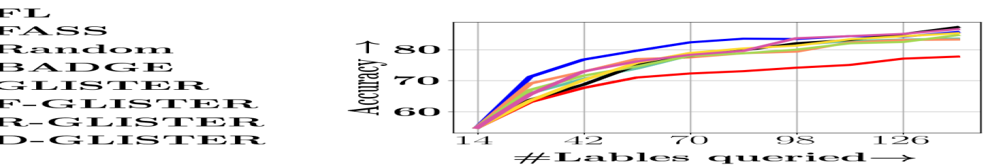


Data Selection for ACTIVE Learning in CLass Imbalance Setting. Datasets: (f) IJCNN1 ClassImb,Third from Top Row: (g) DNA ClassImb, (h) Connect-4 ClassImb, (i) Digits ClassImb, Fourth Row:(j) Letter ClassImb, (k) SatImage ClassImb, (l) USPS ClassImb
Ablation Studies
Convergence with varying L values
In this section, we analyzed the effect of varying values on our model convergence rate on various datasets as shown in the figure 9. From the results, it is evident that our Glister-Online framework has faster convergence for lower values. But using lower values leads to high computational time. This is evident from the results on some datsets where has faster convergence than . Hence, we should be careful about the above trade-off when deciding the value. After extensive analysis, we used in our experiments.


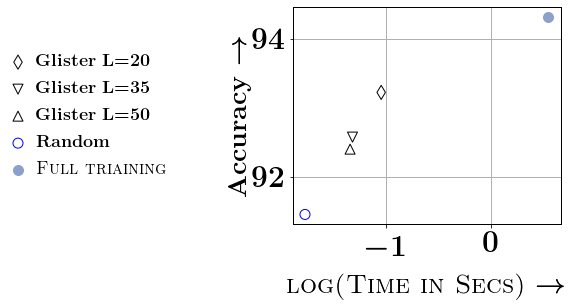

Convergence with varying r values
In this section, we analyzed the effect of varying values on our model convergence rate on various datasets as shown in the figure 10. From the results, it is evident that our Glister-Online framework is highly unstable for low values of and that the stability of our model increases with . But using large values leads to high computational time. Hence, it is not always advisable to use large values. It is also evident from our results shown in figure 10, since our Glister-Online framework has faster convergence when instead of in the majority of the datasets. Hence, after extensive analysis we used in our experiments.


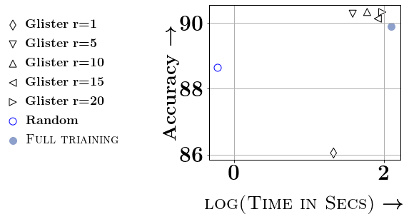
Synthetic Experiments
We specifically designed a set of synthetic data experiments to visualize how the subset selection process of our ”Glister-Online” framework works. Our synthetic datasets include linearly separable binary data, multi-class separable data, and linearly separable binary data with slack. The linearly separable binary dataset, as shown in fig.11(a), comprises two-dimensional feature data points from two non-overlapping data points clusters of class 0 and class 1. The multi-class separable data comprises two-dimensional feature data points from four non-overlapping data points clusters of classes 0,1,2,3 which is shown in fig.12(a). A overlapping version of the same is shown in fig.14(a). Whereas the linearly separable dataset with slack comprises two-dimensional feature data points from two overlapping data points clusters of class 0 and class 1 as shown in fig.13(a).
The result in 11 shows the subset selected by various methods for a linearly binary separable dataset. From fig. 11(b), we can see that our Glister-Online framework selects a subset that is close to the boundary, whereas other methods like CRAIG(Mirzasoleiman, Bilmes, and Leskovec 2020), Random, KNNSubmod (Wei, Iyer, and Bilmes 2015) selects subsets that are representative of the training dataset as shown in figures 11(c), 11(e), 11(d) respectively. Similarly, in fig. 12 points selected by the methods are highlighted for linearly separable dataset with four classes, in figure 13 points selected by the methods are highlighted for binary dataset with outliers and in figure 14 points selected by the methods are highlighted for overlapping dataset with four classes.
From the results shown, it is clearly evident that our Glister-Online Framework tries to select datapoints that are close to the decision boundary where as other methods like CRAIG (Mirzasoleiman, Bilmes, and Leskovec 2020), KNNSubmod (Wei, Iyer, and Bilmes 2015) selects representative points of the whole training set.


Since Glister-Online is driven by validation data, Glister-Online can better handle situations where there is distribution shift in test and validation data from the training data, This what is called as the covariate shift. To illustrate this we use two synthetic datasets which are very similar to dataset, as shown in figure 14(a) and figure 13(a) except that their validation dataset is shifted as shown in figure 15(b) and figure 16(b) respectively. Figures 15(c) and 15(d) shows how effective the methods - CRAIG(Mirzasoleiman, Bilmes, and Leskovec 2020), Random, KNNSubmod (Wei, Iyer, and Bilmes 2015) and Glister-Online are reducing validation and test loss respectively. Clearly Glister-Online outperforms other methods. A similar trend is seen Figures 16(c) and 16(d) for the binary dataset.


