[table] capposition=top
{gongshi,yuzhou}@hust.edu.cn 22institutetext: Baidu Inc., China
GitNet: Geometric Prior-based Transformation for Birds-Eye-View Segmentation
Abstract
Birds-eye-view (BEV) semantic segmentation is critical for autonomous driving for its powerful spatial representation ability. It is challenging to estimate the BEV semantic maps from monocular images due to the spatial gap, since it is implicitly required to realize both the perspective-to-BEV transformation and segmentation. We present a novel two-stage Geometry PrIor-based Transformation framework named GitNet, consisting of (i) the geometry-guided pre-alignment and (ii) ray-based transformer. In the first stage, we decouple the BEV segmentation into the perspective image segmentation and geometric prior-based mapping, with explicit supervision by projecting the BEV semantic labels onto the image plane to learn visibility-aware features and learnable geometry to translate into BEV space. Second, the pre-aligned coarse BEV features are further deformed by ray-based transformers to take visibility knowledge into account. GitNet achieves the leading performance on the challenging nuScenes and Argoverse Datasets.
Keywords:
Birds-Eye-View, Segmentation, Geometric Prior-based1 Introduction
The birds-eye-view (BEV) semantic map is a compact representation of the surrounding environment for autonomous driving, which provides both the layout of road elements and the occupancy of objects. Such representations are useful for downstream tasks such as path planning, collision avoidance. In this work, we focus on BEV map estimation from monocular images.
The BEV semantic segmentation is particularly challenging for two reasons. First, the BEV segmentation implicitly involves two coupled tasks: mapping from perspective view to the birds-eye-view, and pixel-wise classification. Most existing methods [14, 8, 10, 11, 9, 17] learn to convert the image features from the perspective view to the BEV and then perform segmentation. The training process is supervised by the loss function defined in the BEV space alone, and thus the learning procedure of mapping and pixel-wise classification is coupled in these approaches. How to explicitly incorporate the geometry prior knowledge to decouple the feature for mapping and classification remains unexplored. Secondly, a fundamental difference between monocular image segmentation and BEV segmentation lies in that the latter requires inferring the labels of occluded objects behind foreground objects, which places a tremendous difficulty for the network to learn effective feature representation to differentiate the invisible from the visible. In the previous IPM-based methods [19, 23, 13], the features of foreground visible objects occupy the invisible regions in the BEV space. Since the visibility of pixels is not encoded in the features, it is tough for a convolutional neural network to recover the missing information in the invisible regions.
To address the aforementioned concerns, we derive a novel two-stage transformation from the perspective space to the BEV space. In the first stage, we leverage the proposed Geometry-guided Pre-Alignment (GPA) to obtain coarse pre-aligned BEV features. In the GPA, we decouple the BEV segmentation into the perspective image segmentation and geometric prior-based mapping, with explicit supervision by projecting the BEV semantic labels onto the image plane. As the projected labels reflect all ground regions including visible and invisible ones in the perspective view, while the perspective image appearance features only reflect the visible regions, we obtain the visibility-aware image features by fusing the information of projected labels and appearance features. We warp the visibility-aware features into BEV space via the learnable geometry.
In the second stage, the pre-aligned BEV features are further enhanced by the proposed Ray-based Transformer (RT), which adopts the efficient ray-based attention mechanism that we compute the attention map in a single column so as to keep the high-resolution of feature maps. The pre-aligned BEV features conveying appearance and visibility information, along with BEV positional encoding, work as Queries, and the augmented perspective features serve as Keys and Values. Cooperating with the projected labels, the novel Depth-Aware Dice loss is proposed to alleviate the dominant effect by closer instances in perspective view. Besides, since those pixels that have easily-classified appearances or follow a simple perspective-to-BEV mapping, such as most road regions, comprise the majority of the loss, we present a Self-Weighted Dice loss to balance the easy-hard samples among categories. To sum up, the main contributions of our work are as follows:
-
•
We propose a novel two-stage transformation from perspective view to birds-eye-view. In the first stage, we decouple the BEV segmentation into the perspective image segmentation and geometric prior-based mapping, and provide visibility-aware and pre-aligned BEV features. In the second stage, the warped features are deformed by aggregating appearance information.
-
•
We introduce a Depth-aware Dice loss that removes the perspective effect on the perspective image segmentation and a Self-weighted Dice loss to re-weight the easy-hard samples.
-
•
Our framework presents new state-of-the-art performance on two large-scale datasets including nuScenes and Argoverse.
2 Related work
Most BEV segmentation works follow the similar pipeline to first extract features from the monocular image, and then convert the features from the perspective view (PV) to the birds-eye-view (BEV). Based on different PV-BEV transformation strategies, the methods can be grouped into four categories as follows:
IPM-based Methods: An early work [19] performs semantic segmentation in the image plane and then transforms the semantic results into the BEV space via a homography. This approach works well for predicting flat road layout but fails for objects such as cars that stand above the ground plane. [23] alleviates this problem by training a generative adversarial network to refine the predictions from the IPM. More recently [13] transforms the image features into BEV, which is then fed into a deep segmentation network for further refinement.
Depth-based methods: The depth-based methods are one of the main streams in this field. [6] adopts RGB-D images to learn an implicit representation for 3D localization. [18] leverages an in-painting CNN to infer the semantic labels and depths of the scene to obtain the BEV map by projecting the produced semantic point cloud onto the ground plane. EPOSH [5] first performs monocular depth estimation and then exploits depth maps to transform 2D image features to the BEV space. [11, 12, 7, 17] learn a depth distribution within pixels to lift 2D images to 3D point clouds, and then project the point clouds onto BEV space.
Bottleneck-based methods: VED [8] uses the fully-connected bottleneck to realize the transformation, which loses the spatial information. Therefore the output is fairly coarse and fails to segment small objects. VPN [10] predicts the semantic BEV map from a stack of surround-view images, via a fully-connected view-transformer module. PON [14] proposes a column-wise fully-connected layer to realize the transformation of features from image space to BEV space.
Attention based methods: The attention-based methods are attracting increasing attention. NEAT [4] proposes a novel representation termed neural attention fields, which compresses 2D image features into the BEV representation based on the attention map. TIM [16] transforms image columns to BEV polar rays via cross-attention. Though similar to our work, the BEV features are initialized to constant, and the geometric prior is not exploited in their method, which limits the capacity of reasoning in 3D space.
3 Method
In this section, we first briefly present our GitNet approach, which learns the birds-eye-view (BEV) segmentation map from a monocular image . The predicted BEV semantic map is in the ego camera coordinate, with and are the spatial dimensions of the regular lattice grid in BEV space and is the number of semantic categories including road layout and objects.
3.1 Overview

The goal of our network is to predict the semantic map of the scene on the birds-eye-view space from a monocular perspective image. The challenge of predicting the BEV semantic map lies in that the input and output representations exist in different spaces and thus the network is acquired to learn the transformation from perspective image view to orthographic BEV space. As depicted in Fig. 1, our framework is a two-stage pipeline that transforms the perspective view (PV) to the birds-eye-view. It mainly consists of four modules, (i) the feature pyramid network (FPN) for multi-scale perspective feature representation, (ii) Geometry-guided Pre-Alignment that transfers features into BEV space based on the learnable camera height, (iii) the ray-based transformer module for attention-based feature enhancement before BEV segmentation, and (iv) the specially designed loss functions for re-weighting different pixels.
In our network, the core design is the two-stage transformation from the perspective space to the BEV space. Firstly we leverage the geometric guidance to provide appearance and visibility for initializing the transformed BEV features. To solve the ambiguity caused by the mounting height of the camera, we specially learn the height for better alignment between the perspective space and the birds-eye-view space. After obtaining the pre-aligned BEV features, we further adopt the ray-based transformer module based on the column-wise attention for further enhancing the feature deformation in BEV space for conducting semantic segmentation. The explicit supervision is enforced to the GPA Stage guided by the learnable camera height to learn visibility-aware features, which are then converted to pre-aligned BEV features. In addition, to alleviate the perspective effect caused by the imaging, we organize the projected supervision loss in a depth-aware manner and further propose the Self-Weighted Dice (SW-Dice) loss to re-weight the easy-hard samples. We will introduce the detailed design of each component in the following parts.
3.2 Geometry-guided Pre-Alignment

In this section, we introduce the first stage, i.e., the Geometry-guided Pre-Alignment module. We first present the geometric relation between the perspective view and BEV. Then we detail the consistency between image features and projected BEV labels, and describe our visibility-aware feature learning method. Finally, we describe geometry-based warping to obtain the pre-aligned BEV features. The detailed pipeline of this module is depicted in Figure 2.
Learnable Geometric Relation. The transformation from perspective view (PV) to BEV can be given by a projection matrix . We first introduce the coordinate systems: a certain point in the camera coordinate system is represented by . The ground space is by setting the y-coordinate of the camera coordinate system to and a certain point lying on the ground plane turns out to be , where denotes the height of the mounted camera from the ground. The BEV coordinates simply remove the -dim and can be denoted as . In the following, we do not particularly distinguish the BEV space from the ground space in the camera coordinate system. The homogeneous image coordinates have a one-to-one correspondence with the ground coordinates, which can be expressed by:
| (1) |
where is the camera intrinsic matrix: , and the inverse transformation from image to ground coordinates is formulated as:
| (2) |
Based on the geometric correspondences illustrated in the Equation (1) and (2), we are able to transform from the perspective space to the BEV. In this way, we are able to recover the coarse ground coordinates given the image coordinates and the camera height. However, as is acknowledged in [14], the camera height is unavailable for a real monocular perception system. Alternatively, we enforce the network to learn the camera height parameters. The image features with the scale of are compressed into a vector by global average pooling and followed by an MLP to leverage the global context for predicting the offset of the camera height to the empirically predefined height.
Visibility-aware Perspective Feature Learning. The BEV semantic segmentation is an implicit mapping-segmentation coupling task. Here we decouple the BEV segmentation into the geometric prior-based mapping and perspective segmentation. The latter is supervised by an explicit segmentation loss with projecting the BEV GT labels onto the image plane following the transformation in the Equation (1) to generate the projected labels . reflects the whole perspective-view ground including visible or invisible regions. However, the perspective features extracted from images only reflect the visible foreground regions. Therefore, the projected labels can be used to obtain the visibility-aware image features by fusing the information of projected labels and image features. In specific, the pyramid features are separately fed into the weight-shared segmentation head to generate the corresponding probability maps under the supervision of our depth-aware Dice (DA-Dice) segmentation loss with projected labels. We concatenate the feature maps and the corresponding probability maps, and learn the visibility-aware features with pixel-wise fusion (MLP) by:
| (3) |
Geometry-based Warping. From the Equation (2), we can derive that , which indicates that pixels of perspective view lying on the same column (i.e., with the same x-coordinate ) map onto the same polar ray in BEV space with a slope of . Following the transformation in Equation (2), the -th column of augmented image features are warped into the BEV space with the learned camera height by inverse projection. That is:
| (4) |
where are computed in parallel in our implementation, and are concatenated to output the tensor . The warped BEV features take advantage of both the appearance from multi-scale perspective-view features and the visibility with BEV projected-to-PV labels guidance. The geometry-guided transformation module provides initial queries for the follow-up transformer stage for further tuning the features for the BEV segmentation task.
3.3 Ray-based Transformer

The second step of our two-stage transformation pipeline is the ray-based transformer, which is depicted in the Fig. 3. In this stage, we extend the common multi-head attention [21] into our Ray-based Transformer (RT). The multi-head attention needs three inputs of queries , keys , and values , which is denoted as . We refer the reader to the literature [21] and see the appendix for more detailed descriptions. Since our BEV semantic segmentation task requires high-resolution feature maps, computing the attention of a full image, like most existing works, will bring high computation complexity and GPU memory. As derived in Sec. 3.2, pixels of perspective view lying on the same column correspond to the same polar ray of birds-eye-view. This motivates us to compute attention in a single column or ray, which greatly reduces the complexity of attention.
Differences with the Original Transformer. Our method draws on the core idea of Transformer, i.e., employing the multi-head attention mechanism. But we have two new designs for our BEV segmentation task. Firstly, We use column-wise attention so that we can perform on high-resolution feature maps, which is indispensable in our pixel-wise recognition. Secondly, we introduce the pre-aligned features encoding the appearance and visibility, along with BEV positional encoding, as queries in the cross attention. The ablation study in the Sec. 4.3 validates the superiority of our designs. In the following part, we detail two attention mechanisms in our transformer, and omit other components such as normalization for the sake of simplicity. The complete structure can be seen in our supplementary material.
Column Context Augment(CCA) in Encoder. As illustrated in Fig.3, the inputs for the transformer encoders are perspective features extracted from the FPN, where has a spatial resolution of . In the CCA, each pixel adaptively integrates the information from other pixels of the same column, by using multi-head self-attention. We further introduce spatial positional encodings to the input to distinguish the positions of the input features. We use a sine function to generate spatial positional encoding. Let , denote the -th column of and , respectively. The mechanism of CCA can be summarized as
| (5) |
Ray-based Cross-Attention (RCA) in Decoder. RCA in the transformer decoder aims to refine the output of pre-alignment block, , based on the augmented image features . As depicted in Fig.3, the RCA receives the pre-aligned BEV feature as Query, the augmented features built from the encoder as Key and Value. Similar to CCA, spatial positional encoding is also adopted in RCA. The difference is that represents the position in the BEV, while is on the image plane. The mechanism of RCA can be summarized as
| (6) |
Since the columns of are still in the image coordinate, we warp them to rays in the camera coordinate following the transformation in the Equation (2) to obtain , which are responsible for different depth ranges. We concatenate all features along the depth axis to obtain the feature maps of the whole scene:
| (7) |
The final BEV feature maps are fed to the downstream convolutional segmentation network. Thanks to the CCA and RCA-based transformer, the network take appearance and visibility knowledge into account, and further tunes the invisible regions of the pre-aligned BEV features, based on the context information from the perspective features.
3.4 Loss functions
The Dice loss is commonly adopted in segmentation for alleviating the data imbalance problem. The GT semantic label of -th pixel in the BEV map is [, ,…, ], and the predicted probability is [, ,…, ], where and , and is the number of classes. The dice loss can be formulated as:
| (8) |
where is the number of pixels in a mini-batch and is a constant used to prevent division by zero.
For the BEV semantic segmentation task which is actually an implicit multi-task problem involving 3D location and segmentation, there are two problems that can affect the performance. For one thing, due to the perspective projection from the real world to the image plane, distant objects appear to be smaller than nearer objects. In other words, the closer instances occupy much more pixels than farther ones, which dominate the overall segmentation loss in the perspective view. For another, those pixels that have easily-classified appearances or follow a simple perspective-to-BEV mapping, such as most road regions, comprise the majority of the loss.
Occlusion-free Depth-aware Dice Loss: As discussed in Sec. 3.2, we project the BEV labels onto the image plane to generate the projected labels , which supervises the segmentation on the perspective view. To tackle the first problem caused by the domination of nearer objects in perspective images, we propose the novel Depth-aware Dice loss by re-weighting the loss in a depth-aware manner. In specific, the Jacobian determinant gives the ratio of the area ratio between image ground plane () and the BEV ground plane () as:
| (9) |
We find that the area ratio is proportional to , thus we re-weight the pixels with the weight to solve the imbalance. The depth-aware dice loss is:
| (10) |
Self-Weighted Dice Loss: To further alleviate the second problem, i.e., the dominating influence from easy samples in training, we propose to associate training samples with dynamically adjusted weights to emphasize hard examples. We first propose a weighting function to adjust the hard-mining strength by a parameter in Equation (11) and then utilize to reweight the Dice loss and obtain the self-weighted dice loss in Equation (12).
| (11) |
| (12) |
Note that we detach the weighting function to stop the backward propagation of the gradient in Equation (12). Otherwise, the term within will be maximized to make fall around the undesired value 0.5.
4 Experiments
4.1 Experimental Setup
Dataset We conduct extensive experiments on two large-scale datasets: The nuScenes [1] and Argoverse [3] road-scene datasets. Since the two datasets are predominantly collected for 3D object detection task rather than BEV semantic segmentation task, we follow the data generation method in [14] to convert the ground truth 3D bounding box annotations and the vectorized road maps into GT semantic maps in BEV. In addition, for fair comparisons, we also follow the same training and validation splits with other methods. The nuScenes includes 4 road layout categories and 7 object categories, and the Argoverse includes 7 object categories as well as drivable road. For both datasets, the ground truth of birds-eye-view expands from 1m to 50m in front of the camera i.e., along the -direction and 25m to either side (i.e., along the -direction). Due to the greater diversity of nuScenes, we choose this dataset for all ablation studies.
Implementation details For fair comparisons, we adopt a pretrained ResNet-50 with a feature pyramid on top as the backbone. We adopt a simplified HRNet [22] as the BEV segmentation head. In our implementation, we use a simplified HRNet32 by halving the number of blocks in each stage. We use two encoder layers and four decoder layers in the Ray-based transformer. The hyperparameter in Equation 11 for the SW-Dice loss is set as 0.5. We adopt a similar depth-interval assignment strategy with [14], but we only use the former four scales of the FPN. The concatenated BEV feature maps from different depth intervals are of pixels, with each pixel covering 0.5m. We obtain the final output map with a resolution of pixels by upsampling, which is consistent with other methods. The model is trained using four Tesla V100 cards, each with 32G memory. We optimize the network with Adam policy for gradients accumulated over every 8 iterations and train for 40 epochs. The initial learning rate is set to 0.0002, with a weight decay of 0.99 and batch size 12.
Evaluation metric Our evaluation metric is the Intersection over Union (IoU) score, which we compute by binarizing the output probability maps with the threshold of 0.5. Invisible regions are ignored during evaluation following [14].
| Method | Layout | Object | Mean | ||||||||||||
|---|---|---|---|---|---|---|---|---|---|---|---|---|---|---|---|
| Drivable | Crossing | Walkway | Carpark | Bus | Bike | Car | C.V. | Motor. | Trailer | Truck | Ped. | Cone | Barrier | ||
| IPM [14] | 40.1 | - | 14.0 | - | 3.0 | 0.2 | 4.9 | - | 0.8 | - | - | 0.6 | - | - | - |
| Depth Unpr.[14] | 27.1 | - | 14.1 | - | 6.7 | 1.3 | 11.3 | - | 2.8 | - | - | 2.2 | - | - | - |
| VED [8] | 54.7 | 12.0 | 20.7 | 13.5 | 0.0 | 0.0 | 8.8 | 0.0 | 0.0 | 7.4 | 0.2 | 0.0 | 0.0 | 4.0 | 8.7 |
| VPN [10] | 58.0 | 27.3 | 29.4 | 12.3 | 20.0 | 4.4 | 25.5 | 4.9 | 5.6 | 16.6 | 17.4 | 7.1 | 4.6 | 10.8 | 17.5 |
| Sim2real [13] | 60.5 | 27.1 | 19.2 | 18.3 | 6.9 | 3.8 | 7.1 | 0.3 | 4.5 | 3.2 | 4.7 | 1.8 | 4.2 | 12.1 | 12.4 |
| OFT [15] | 62.4 | 30.9 | 34.5 | 23.5 | 23.2 | 4.6 | 34.7 | 3.7 | 6.6 | 18.2 | 17.3 | 1.2 | 1.1 | 12.9 | 19.6 |
| PON [14] | 60.4 | 28.0 | 31.0 | 18.4 | 20.8 | 9.4 | 24.7 | 12.3 | 7.0 | 16.6 | 16.3 | 8.2 | 5.7 | 8.1 | 19.1 |
| STA-S [17] | 71.1 | 31.5 | 32.0 | 28.0 | 22.8 | 14.6 | 34.6 | 10.0 | 7.1 | 11.4 | 18.1 | 7.4 | 5.8 | 10.8 | 21.8 |
| EPOSH [5] | 61.1 | 33.5 | 37.8 | 25.4 | 31.8 | 6.7 | 37.8 | 2.7 | 10.5 | 14.2 | 20.4 | 5.9 | 7.6 | 13.4 | 22.1 |
| Ours | 65.1 | 41.6 | 42.1 | 31.9 | 35.4 | 13.8 | 43.4 | 9.7 | 15.0 | 22.5 | 25.5 | 14.1 | 11.6 | 18.6 | 27.9 |

4.2 Main Results
We evaluate our method on nuScenes and Argoverse, and compare against the recently published works which belong to different branches: (i) IPM-based methods: IPM [14], Sim2real [13]; (ii) Bottleneck-based methods: VED [8], VPN [10] and PON [14]; (iii) Depth-based methods: Depth Unprojection-based (Depth-Unpr.) [14], OFT [15], EPOSH [5] and STA-S [17]. All these works report the results on nuScenes as shown in Table 1, or provide the results on Argoverse in Table 2. Among all these methods, our method achieves the best performance for most categories and our method surpasses the previous approaches with a significant margin of mean IoU, 6.1% and 3.2% on nuScenes and Argoverse, respectively. Fig. 8 further shows the visual comparisons against other methods on the nuScenes Dataset. The two fully-connected bottleneck-based works, VPN and VED, achieve a comparable IoU on the road drivable area, but they fail to recognize the smaller objects such as vehicles due to the image features are compressed into a vector. In contrast, our method leverages multi-scale spatial information for different depth intervals to keep the fine details. For example, as shown in Fig. 8, our approach accurately predicts the vehicles within all depth ranges. Compared with other relatively better methods like PON and STA-S, we exploit the geometric prior which helps to accurately locate and identify the road elements, like walkway and pedestrian crossing, which is supported by the qualitative results in Fig. 8.
| Method | Drivable | Vehicle | Ped. | Large veh. | Bicycle | Bus | Trailer | Motorcy. | Mean |
|---|---|---|---|---|---|---|---|---|---|
| IPM [14] | 43.7 | 7.5 | 1.5 | - | 0.4 | 7.4 | - | 0.8 | - |
| Depth Unpr.[14] | 33.0 | 12.7 | 3.3 | - | 1.1 | 20.6 | - | 1.6 | - |
| VED [8] | 62.9 | 14.0 | 1.0 | 3.9 | 0.0 | 12.3 | 1.3 | 0.0 | 11.9 |
| VPN [10] | 64.9 | 23.9 | 6.2 | 9.7 | 0.9 | 3.0 | 0.4 | 1.9 | 13.9 |
| PON [14] | 65.4 | 31.4 | 7.4 | 11.1 | 3.6 | 11.0 | 0.7 | 5.7 | 17.0 |
| Ours | 67.1 | 35.9 | 9.8 | 15.7 | 4.9 | 31.7 | 11.3 | 6.2 | 20.2 |
4.3 Ablation Study
We conduct ablation studies to evaluate the key designs in our method. Unless otherwise specified, we evaluate on the nuScenes validation set. GPA denotes Geometry-guided Pre-Alignment, and RT is the Ray-based Transformer for short.
| Group | Network | Loss | mIoU (%) | ||||
|---|---|---|---|---|---|---|---|
| GPA | RT | SW | DA | Layout | Object | Total | |
| (a) | 31.2 | 4.9 | 12.4 | ||||
| (b) | ✓ | 38.7 | 15.4 | 22.1 | |||
| (c) | ✓ | 40.6 | 16.8 | 23.6 | |||
| (d) | ✓ | ✓ | 43.2 | 19.1 | 26.0 | ||
| (e) | ✓ | ✓ | ✓ | 43.8 | 19.9 | 26.7 | |
| (f) | ✓ | ✓ | ✓ | 44.1 | 20.5 | 27.2 | |
| (g) | ✓ | ✓ | ✓ | ✓ | 45.2 | 21.0 | 27.9 |
Effects of different components. To analyze the effects of the key designs, we try different combinations and summarize the ablation results in Table 3.
-
Baseline. Group (a) is the baseline that is similar to [13]. We transform the image features onto the ground plane via a homography matrix. The difference between it and our GPA is that it adopts a fixed camera height and is not supervised by the projected semantic maps. The transformed features are further processed by a segmentation network that is the same as our best model for fair comparisons. From Row 1 in Table 3, we can see that the baseline achieves reasonable results in road layout areas, but fails to distinguish the objects that standing above the road.
-
Network. In Group (b), the GPA provides a reliable prior for feature transformation and relieves the effects of occlusion by supervision of projection, improving the mIoU by +9.7% in total. The RT (c) transforms the image features to the BEV space by multi-scale column-based attention, which improves the mIoU by +11.2% in total. If we combine the GPA and RT as disscussed in Sec. 3.1, their joint effect (d) further enhances the performance by +13.6% in total. It shows the geometric prior provides complementary information for the RT.
-
Loss. Groups (e)(f)(g) show the improvements in our proposed loss function. The SW-Dice loss (e) automatically puts higher weights on these pixels that are hard to classify in birds-eye-view, improving the mIoU by +0.7% in total. The DA-Dice loss (f) balances the pixels of different depth ranges in the perspective view by reweighting the Dice loss under the guidance of the cubic depth when learning the geometric prior-based pre-alignment module, which improves the mIoU by +1.2% in total. The joint of both losses (g) brings a further mIoU gain of +1.9% in total.
| Group | learnable | proj. sup. | pixel. fusion | Layout | Object | Total |
|---|---|---|---|---|---|---|
| I | 40.2 | 16.7 | 23.4 | |||
| II | ✓ | 41.1 | 17.3 | 24.1 | ||
| III | ✓ | ✓ | 42.6 | 18.3 | 25.2 | |
| IV | ✓ | ✓ | ✓ | 43.2 | 19.1 | 26.0 |
Effects of components of GPA: Three key designs are presented in Geometry-guided Pre-Alignment to better convert the perspective image features to BEV features, including the learnable camera height, the projection supervision, and pixel-wise fusion between probability maps and image features. Comparing Group I and II, where we enforce the network to learn the offset of the camera height, we observe a 0.7% mIoU gain. Group III leverages the projected labels from BEV space to image space to supervise the feature learning procedure, which further improves the performance by 1.1% mIoU. The further pixel-wise fusion between perspective features and segmentation probability maps in Group IV further lifts the performance, resulting in a total of 2.6% gain.
| 0 | 0.25 | 0.5 | 1.0 | 2.0 | |
|---|---|---|---|---|---|
| Layout | 44.1 | 44.2 | 45.2 | 45.3 | 45.1 |
| Object | 20.5 | 20.9 | 21.0 | 20.9 | 20.6 |
| Total | 27.2 | 27.5 | 27.9 | 27.9 | 27.6 |
| layers | 0 | 1 | 2 | 3 | 4 |
|---|---|---|---|---|---|
| Layout | 38.7 | 43.7 | 44.1 | 44.8 | 45.2 |
| Object | 15.4 | 19.2 | 20.8 | 21.2 | 21.0 |
| Total | 22.1 | 26.2 | 27.5 | 27.9 | 27.9 |
Effects of in SW-Dice loss: The SW-Dice loss introduces the hyperparameter to control the strength of the modulating term with respect to the predicted probability. As is shown in Table 5(a), means our loss is equivalent to the plain Dice loss. As increases, the predicted probability gets dominant in the weighting function. Under all settings of , the proposed SW-Dice loss stably outperforms the baseline (). With the best setting, the SW-Dice loss yields a 0.7% improvement over the plain Dice loss.
Effects of decoder layers in RT: Table 5(b) shows the performance with various number of decoder layers within the ray-based transformer. Our model can yield 4.1% improvement even using one layer. The gain reflects that the pre-aligned BEV features can provide a good initialization for the decoder. With the decoder layers increasing, higher performance can be achieved. We observe that it becomes saturated when adopting more than three layers.
4.4 Multiple Views Fusion
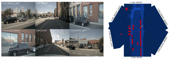
Due to the limited field of view (FOV) of a single camera, it is essential to make full use of all surrounding cameras from multi-view to perceive the integrated scope of the scene. For this purpose, we introduce a late-fusion technique based on Bayesian filtering [14, 20]. Suppose that and are the BEV rotation and translation matrix of -th camera with respect to the ego car coordinates. Let denote the predicted logits (before the sigmoid activation) in -th view. is warped to the car coordinate system, and we sum over all warped logits maps. The sum of logits are normalized by the sigmoid function to output the fused probability map . In Fig. 5, we give an example of the fused 360∘ BEV semantic maps from six surround-view cameras. It validates that our approach can be applied seamlessly to predict consistent maps across views.
5 Conclusion
In this paper, we proposed a novel method GitNet for predicting semantic birds-eye-view maps from monocular images. The GitNet leverages a two-stage pipeline to transform the perspective view into the birds-eye-view, which first performs geometry-guided pre-alignment and then further enhances the BEV features based on ray-based transformers. Our approach can also be easily adapted to multi-view scenarios to build a full-scene BEV map.
Acknowledgments. This research was supported by the National Key Research and Development Program of China under Grant No. 2018AAA0100400, the National Natural Science Foundation of China (62176098, 61703049) and the Natural Science Foundation of Hubei Province of China under Grant 2019CFA022.
References
- [1] Caesar, H., Bankiti, V., Lang, A.H., Vora, S., Liong, V.E., Xu, Q., Krishnan, A., Pan, Y., Baldan, G., Beijbom, O.: nuscenes: A multimodal dataset for autonomous driving. In: Proceedings of the IEEE/CVF Conference on Computer Vision and Pattern Recognition(CVPR). pp. 11621–11631 (2020)
- [2] Carion, N., Massa, F., Synnaeve, G., Usunier, N., Kirillov, A., Zagoruyko, S.: End-to-end object detection with transformers. In: European Conference on Computer Vision(ECCV). pp. 213–229 (2020)
- [3] Chang, M.F., Lambert, J., Sangkloy, P., Singh, J., Bak, S., Hartnett, A., Wang, D., Carr, P., Lucey, S., Ramanan, D., et al.: Argoverse: 3d tracking and forecasting with rich maps. In: Proceedings of the IEEE/CVF Conference on Computer Vision and Pattern Recognition(CVPR). pp. 8748–8757 (2019)
- [4] Chitta, K., Prakash, A., Geiger, A.: Neat: Neural attention fields for end-to-end autonomous driving. In: Proceedings of the IEEE/CVF International Conference on Computer Vision(ICCV). pp. 15793–15803 (2021)
- [5] Dwivedi, I., Malla, S., Chen, Y., Dariush, B.: Bird’s eye view segmentation using lifted 2d semantic features. In: 32nd British Machine Vision Conference(BMVC). p. 383 (2021)
- [6] Henriques, J.F., Vedaldi, A.: Mapnet: An allocentric spatial memory for mapping environments. In: Proceedings of the IEEE Conference on Computer Vision and Pattern Recognition(CVPR). pp. 8476–8484 (2018)
- [7] Hu, A., Murez, Z., Mohan, N., Dudas, S., Hawke, J., Badrinarayanan, V., Cipolla, R., Kendall, A.: Fiery: Future instance prediction in bird’s-eye view from surround monocular cameras. In: Proceedings of the IEEE/CVF International Conference on Computer Vision(ICCV). pp. 15273–15282 (2021)
- [8] Lu, C., van de Molengraft, M.J.G., Dubbelman, G.: Monocular semantic occupancy grid mapping with convolutional variational encoder–decoder networks. IEEE Robotics and Automation Letters 4(2), 445–452 (2019)
- [9] Mani, K., Daga, S., Garg, S., Narasimhan, S.S., Krishna, M., Jatavallabhula, K.M.: Monolayout: Amodal scene layout from a single image. In: Proceedings of the IEEE/CVF Winter Conference on Applications of Computer Vision(WACV). pp. 1689–1697 (2020)
- [10] Pan, B., Sun, J., Leung, H.Y.T., Andonian, A., Zhou, B.: Cross-view semantic segmentation for sensing surroundings. IEEE Robotics and Automation Letters 5(3), 4867–4873 (2020)
- [11] Philion, J., Fidler, S.: Lift, splat, shoot: Encoding images from arbitrary camera rigs by implicitly unprojecting to 3d. In: European Conference on Computer Vision(ECCV). pp. 194–210 (2020)
- [12] Reading, C., Harakeh, A., Chae, J., Waslander, S.L.: Categorical depth distribution network for monocular 3d object detection. In: Proceedings of the IEEE/CVF Conference on Computer Vision and Pattern Recognition(CVPR). pp. 8555–8564 (2021)
- [13] Reiher, L., Lampe, B., Eckstein, L.: A sim2real deep learning approach for the transformation of images from multiple vehicle-mounted cameras to a semantically segmented image in bird’s eye view. In: 2020 IEEE 23rd International Conference on Intelligent Transportation Systems(ITSC). pp. 1–7 (2020)
- [14] Roddick, T., Cipolla, R.: Predicting semantic map representations from images using pyramid occupancy networks. In: Proceedings of the IEEE/CVF Conference on Computer Vision and Pattern Recognition(CVPR). pp. 11138–11147 (2020)
- [15] Roddick, T., Kendall, A., Cipolla, R.: Orthographic feature transform for monocular 3d object detection. In: 30th British Machine Vision Conference(BMVC). p. 285 (2019)
- [16] Saha, A., Maldonado, O.M., Russell, C., Bowden, R.: Translating images into maps. arXiv preprint arXiv:2110.00966 (2021)
- [17] Saha, A., Mendez, O., Russell, C., Bowden, R.: Enabling spatio-temporal aggregation in birds-eye-view vehicle estimation. In: 2021 IEEE International Conference on Robotics and Automation (ICRA). pp. 5133–5139 (2021)
- [18] Schulter, S., Zhai, M., Jacobs, N., Chandraker, M.: Learning to look around objects for top-view representations of outdoor scenes. In: Proceedings of the European Conference on Computer Vision(ECCV). pp. 787–802 (2018)
- [19] Sengupta, S., Sturgess, P., Ladickỳ, L., Torr, P.H.: Automatic dense visual semantic mapping from street-level imagery. In: 2012 IEEE/RSJ International Conference on Intelligent Robots and Systems. pp. 857–862 (2012)
- [20] Thrun, S.: Probabilistic robotics. Communications of the ACM 45(3), 52–57 (2002)
- [21] Vaswani, A., Shazeer, N., Parmar, N., Uszkoreit, J., Jones, L., Gomez, A.N., Kaiser, Ł., Polosukhin, I.: Attention is all you need. Advances in Neural Information Processing Systems(NIPS) 30 (2017)
- [22] Wang, J., Sun, K., Cheng, T., Jiang, B., Deng, C., Zhao, Y., Liu, D., Mu, Y., Tan, M., Wang, X., et al.: Deep high-resolution representation learning for visual recognition. IEEE Transactions on Pattern Analysis and Machine Intelligence(TPAMI) 43(10), 3349–3364 (2020)
- [23] Zhu, X., Yin, Z., Shi, J., Li, H., Lin, D.: Generative adversarial frontal view to bird view synthesis. In: 2018 International conference on 3D Vision(3DV). pp. 454–463 (2018)
Appendix 0.A Ray-based Transformer
0.A.1 Detailed architecture
The detailed description of the Ray-based Transformer adopted in GitNet, with positional encodings passed at each attention layer, is given in Fig. 6. The perspective image features , i.e., the -th column of the -th level of pyramid features, are passed through the transformer encoder (Column Context Augment, CCA), together with perspective positional encoding that are added to queries and keys at every multi-head self-attention layer. Then, the decoder (Ray-based Cross-Attention, RCA) receives queries, that are initialized as the pre-alined features , along with the BEV positional encoding, and the output of encoder , along with the perspective positional encoding, and produces the refined features through multi-head cross-attention.

0.A.2 Positional Encoding
2D positional encoding As the transformer is unable to distinguish the position of elements, we add positional encoding to the Keys and Queries following [2, 21]. The 2D positional encoding map have the same shape with the input features, that denotes as , where is the channel number, and are the height and width of input features, at horizontal and vertical direction, respectively. We encode horizontal position in the first half of channels, and the vertical positions in the second half channels. Suppose the and denotes the row and column index, then the horizontal positional encoding at the point of is:
| (13) |
The vertical positional encoding is:
| (14) |
Where is the channel index. We concatenate the positional encoding at two directions to get the whole 2D positional encoding, that is . PV and BEV positional encoding Both our perspective-view (PV) and birds-eye-view (BEV) positional encoding follow the paradigm of 2D positional encoding detailed above. The only difference is that PV positional encoding has the same spatial size with image features, while the BEV positional encoding has spatial size of rasterized BEV map.

0.A.3 What does the cross-attention see?
To explore how the cross-attention module works in our framework, we visualized the attention maps of a representative sample, as shown in Fig. 7. As our ray-based transformer computes the cross-attention between every query point in the BEV and the corresponding column of the perspective image features, a lateral query line cross all columns/rays (white query line in Fig. 7) produces the attention maps of the full perspective image features. We depict the cross-attention map from three different decoder layers, which go deeper from left to right. In the first row, the queries lie on the pedestrian crossing, 10 meters away from the camera, and in the right three columns, we can observe that the corresponding cross-attention maps mainly focus on the pedestrian crossing region of the perspective space. When the queries line move farther,20 meters away, the attention maps focus on upper regions of the perspective images. Since our pre-alignment module provides visibility-aware pre-aligned features to the transformer, the invisible regions can be further refined by aggregating contextual information from other visible regions. This can be supported by the observation that the attention maps of invisible regions tend to disperse over an extensive region, while attentions maps of visible ground mostly focus a certain point. In the fourth row, the query line is 40 meters away, and the attention maps are scattered in the invisible regions that occluded by the building and cars.

Appendix 0.B Robustness under Different Conditions
In Fig. 8, we depict additional visualization results by selecting samples from the validation set of nuScenes including three different weather conditions: light, rainy and dark. For the purpose of practical use, our model must be able to handle these various conditions. From the Fig. 8, our model can perform well in the light conditions (the first group), and under the more challenging rainy condition (the second group), our model can segment almost all other cars and the complete layout of the crossroads. Under the dark condition (the third group), our model also succeed to segment the forwarding cars, and right sidewalk which cannot be seen clearly even for human.