$g+ig$ topological superconductivity in the 30°-twisted bilayer graphene

Introduction: The twisted multi-layer graphene family since synthesis have driven the revelation of such intriguing quantum phases caoyuan20181 ; caoyuan20182 ; Yankowitz2019 ; Dean2019 ; Yazdani2019 ; Efetov2019 ; David2019 ; Serlin2019 ; P_Kim2020 ; Zeldov2020 ; P_Kim2021 ; Caoyuan2021 as the superconductivity (SC), the correlated insulator, the nematic phase, the quantum anomalous Hall, etc, which have aroused great research interests Xu2018 ; Po2018 ; Yuan2018 ; YangFan2018 ; WuFeng20181 ; Kang2018 ; Isobe2018 ; Koshino2018 ; Fernandes2018 ; Kang2019 ; Po2019 ; Dai2019 ; Honerkamp20191 ; Gonzalez2019 ; Song2019 ; Ahn2019 ; Angeli2019 ; Lian2019 ; Jiangpeng2019 ; Vishwanath2019prl ; Linyuping2019 ; MingXie2020 ; Abouelkomsan2020 ; Bultinck2020prx ; Senthil2020 ; Liao2021 ; Chichinadze2020 ; Mohammad2020 ; Wuxianxin2020 . While most of these studies are focused on the low twist-angle regimes, here we consider the recently synthesized Ahn2018 ; Yao2018 ; Pezzini2020 ; Yan2019 ; Deng2020 30°-twisted bilayer graphene (TBG). This quasi-crystal TBG (QC-TBG) system hosts no real-space period and is characterized by an exact dodecagonal rotation symmetry verified by various experimentsAhn2018 ; Yao2018 ; Pezzini2020 ; Yan2019 ; Deng2020 . While the single-particle properties of this material have been widely studiedAhn2018 ; Yao2018 ; Moon2013 ; Koshino2015 ; Moon2019 ; Park2019 ; Crosse2021 ; Yuanshengjun2019 ; Yuanshengjun20201 ; Yuanshengjun20202 ; Aragon2019 , physical properties driven by electron-electron (e-e) interaction have not been investigated. Here we focus on possible exotic pairing states in the doped QC-TBG.

It has been long to search SC in the graphene family. Particularly, various groups have proposed Doniach2007 ; Gonzalez2008 ; Honerkamp2008 ; Pathak2010 ; McChesney2010 ; Nandkishore2012 ; Wang2012 ; Kiesel2012 ; Honerkamp2014 that the chiral $d_{x^{2}-y^{2}}\pm id_{xy}$ (abbreviated as $d+id$ below) topological SC (TSC) can be driven in the mono-layer graphene by e-e interaction near the van Hove (VH) doping. Recently, this material has been successfully doped to the beyond-VH regime exp_VHS , which puts on the agenda the search of the exotic $d+id$ chiral TSC. It’s timely now to investigate what exotic pairing states can be induced by the Josephson coupling between the $d+id$ pairing order parameters in the two mono-layers in the QC-TBG. While such weak inter-layer Josephson coupling is not expected to significantly change the $T_{c}$, certain choice of the relative phase difference between the two pairing order parameters can lead to new irreducible representation (IRRP) of the enlarged point group in QC-TBG, and hence novel TSC. Generally, TSCs on periodic lattices with at most 6- folded rotation axes can be generated from 2D $E_{1}$ ($p+ip$) or $E_{2}$ ($d+id$) IRRPs of the point groups. However, the dodecagonal rotation symmetry in the QC-TBG allows for more 2D IRRPs and hence more novel TSCs with higher pairing angular momenta $L\geq 3$.

On the other front, the SC on QCs has recently been a hot topic DeGottardi2013 ; YuPeng2013 ; Loring2016 ; Sakai2017 ; Andrade2019 ; Sakai2019 ; Varjas2019 ; Nagai2020 ; Caoye2020 ; Sakai2020 ; YYZhang2020 ; Hauck2021 ; Zhoubin2021 , particularly after the synthesis of the QC Al-Zn-Mg superconductor exp . Presently, most of these studies are focused on the intrinsic QC such as the Penrose lattice. Instead, the QC-TBG belongs to extrinsic QC Moon2019 which hosts two perfect crystal layers with independent periods, wherein the quasi-periodic nature appears only in the perturbational coupling between the two layers. This structural character enables us to treat the system in the $\mathbf{k}$- space via the perturbational band theory, which lends us more convenience and insight to understand the SC on the extrinsic QC. Besides, it’s interesting to clarify the difference between the pairing natures on intrinsic and extrinsic QCs.

In this paper, we study the pairing states in the doped QC-TBG, adopting the t-J model on this QC. We revise the perturbational band theory to suit it to the study on the finite lattice involving e-e interaction. The mean-field (MF) pairing phase diagram in the low electron-doped regime shows that the beneath-VH and beyond-VH doping regimes are covered by the $d+id$ and $g+ig$ TSCs, respectively. The $g+ig$ TSC belongs to the 2D $E_{4}$- IRRP of the effective $D_{12}$ point group unique to this QC, which possesses a high $L=4$ and its gap phase changes $2\pi/3$ for each 30$\degree$- rotation. Such an intriguing TSC originates from the Josephson coupling between the $d+id$ pairings on the two monolayers, as suggested by the Ginzburg-Landau theory. Our results not only open the door to study e-e correlation driven phases on extrinsic QCs, but also reveal a novel TSC rare on periodic lattices.

Model and Approach: We start from the following tight-binding (TB) model for the QC-TBGMoon2019 ,

with $t_{\mathbf{ij}}$ provided in the SMSM adopted from Ref. Moon2019 . Eq. (S1) can be decomposed into the zeroth-order intra-layer hopping term $H_{0}$ and the perturbational inter-layer tunneling term $H^{\prime}$ as

Here $\mathbf{k}/\mathbf{q}$, $\mu(=\text{t(top)},\text{b(bottom)})$, $\alpha/\beta$ and $\sigma$ label the momentum, layer, band and spin respectively, $\varepsilon_{\mathbf{k}}^{\mu\alpha}$ is the monolayer dispersion and $T^{\alpha\beta}_{\mathbf{kq}}$ is given byMacDonald2011 ; Castro2007 ; Castro2012 ; Bistritzer2010 ; Moon2013 ; Koshino2015 ; Moon2019

In thermal dynamic limit, the nonzero $T^{\alpha\beta}_{\mathbf{kq}}$ requires $\mathbf{k}+\mathbf{G}^{(\text{t})}=\mathbf{q}+\mathbf{G}^{(\text{b})}$Ahn2018 ; Yao2018 ; Moon2013 ; Koshino2015 ; Moon2019 , where $\mathbf{G}^{(\text{t/b})}$ represent the reciprocal lattice vectors for the t/b layers. Under this condition, we have $T^{\alpha\beta}_{\mathbf{kq}}\propto t\left(\mathbf{k}+\mathbf{G}^{(\text{t})}\right)$, which decays promptly with $|\mathbf{k+G}^{(\text{t})}|$. Therefore each zeroth-order top-layer eigenstate $\left|\mathbf{k}\alpha^{(\text{t})}\right\rangle$ can only couple with a few isolated bottom-layer eigenstates $\left|\mathbf{q}\beta^{(\text{b})}\right\rangle$, and vice versa, which justifies the perturbational treatment.

Note that on our finite lattice with discrete momentum points, for each typical $\mathbf{k}$ on the top layer, no $\mathbf{q}$ on the bottom layer can make $\mathbf{k}+\mathbf{G}^{(\text{t})}=\mathbf{q}+\mathbf{G}^{(\text{b})}$ exactly satisfied. Therefore for each top-layer state $|\mathbf{k}\alpha^{(\text{t})}\rangle$, we abandon this relation and directly use Eq. (3) to find the bottom-layer states $|\mathbf{q}_{i}\beta_{i}^{(\text{b})}\rangle$ which obviously couple with it. Then, for these $|\mathbf{q}_{i}\beta_{i}^{(\text{b})}\rangle$ states, we find again all the $|\mathbf{k}^{\prime}_{j}\alpha_{j}^{(\text{t})}\rangle$ states which obviously couple with them. Gathering all these states related to $|\mathbf{k}\alpha^{(\text{t})}\rangle$ as bases to form a close sub-space, we can write down and diagonalize the Hamiltonian matrix in this sub-space to obtain all the eigen states. Among these states, the one having the largest overlap with $|\mathbf{k}\alpha^{(\text{t})}\rangle$ is marked as its perturbation-corrected state $|\widetilde{\mathbf{k}\alpha^{(\text{t})}}\rangle$, whose energy is marked as $\tilde{\varepsilon}^{\text{t}\alpha}_{\mathbf{k}}$. The procedure to get $|\widetilde{\mathbf{q}\beta^{(\text{b})}}\rangle$ and $\tilde{\varepsilon}^{\text{b}\beta}_{\mathbf{q}}$ is similar. For more details, see the Supplementary Material (SM)SM . The approach developed here is a finite-lattice version of the second-order perturbational theory in Ref. Yao2018 ; Moon2013 ; Koshino2015 .

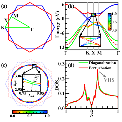
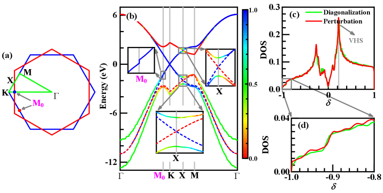
Along the lines connecting the high-symmetry points in the Brillouin zone marked in Fig. 1 (a), we plot our obtained band structure (solid lines) in Fig. 1 (b), in comparison with the uncoupled band structures (dashed lines) from the two layers. Remarkably, while there is obvious band splitting caused by inter-layer hybridization on the hole-doped side, the band structure on the electron-doped side is overall not far from simply overlaying the two uncoupled monolayer band structures, reflecting the much weaker inter-layer hybridization thereKoshino2015 ; Moon2019 , proved in the SMSM . Below, we shall focus on the electron-doped side as the weaker inter-layer coupling there validates our perturbational approach.

The main effect of the inter-layer coupling on the electron-doped side lies in that the top-layer band branches and the bottom-layer ones cross and split at the $X$ points, and simultaneously their layer components are exchanged (see the inset of Fig. 1 (b)). Actually, such band crossing and splitting takes place on all the $\Gamma$-$X$ lines: For each $\mathbf{k}$ on these lines, by symmetry, the states $|\mathbf{k}\alpha^{(\text{t})}\rangle$ and $|\mathbf{k}\alpha^{(\text{b})}\rangle$ possess degenerate zeroth-order energy. They are further coupled via $\mathbf{k}+\mathbf{G}^{(\text{t})}=\mathbf{k}+\mathbf{G}^{(\text{b})}$ by setting $\mathbf{G}^{(\text{t})}=\mathbf{G}^{(\text{b})}=0$, leading to their hybridization and the resulting band splitting. Consequently, the FSs contributed from the two layers also cross and split upon crossing these lines, and simultaneously the layer components are exchanged, see Fig. 1 (c). The emergent FSs with dodecagonal symmetry can be viewed as the inter-layer bonding- and anti-bonding- FSs.

The density of state (DOS) obtained by our approach is well consistent with that obtained by directly diagonalizing the real-space Hamiltonian, particularly in the electron-doped side, as shown in Fig. 1(d). We have further checked that the obtained set of states $\{|\widetilde{\mathbf{k}\alpha^{(\mu)}}\rangle\}$ are almost mutually orthogonal. These properties well qualify them as a good set of single-particle bases for succeeding studies involving e-e interaction.

Now we come to the e-e interaction. As the local Hubbard $U$ for the graphene family can vary from 10 eV to 17 eVgraphene_RMP , comparable with the total band width $W_{b}\approx 18$ eV, the weak-coupling approach might not be suitable here. For simplicity, we take the strong-coupling limit, wherein the strong on-site repulsion induces the following superexchange interaction

with $J_{\mathbf{ij}}=4t_{\mathbf{ij}}^{2}/U$ and $U=10$ eV. Here the sum $\sum_{(\mathbf{i,j})}$ goes through the $(\mathbf{i,j})$ pairs on the bilayer. The total Hamiltonian is then given by the following t-J model,

Eq. (5) is solved in the SMSM by the MF or the Gutzwiller MF approaches, which yield the same pairing symmetry. Focusing on the intra-band pairing between opposite momenta, we obtain the pairing potential $V^{\mu\alpha}_{\nu\beta}(\mathbf{k},\mathbf{q})$ and the linearized gap equation near $T_{c}$,

Here $\tilde{\xi}_{\mathbf{i},\mathbf{k}\mu\alpha}/\sqrt{N}$ denotes the wave function of $|\widetilde{\mathbf{k}\alpha^{(\mu)}}\rangle$, $v_{F}^{\nu\beta}(\mathbf{q})$ is the Fermi velocity and $q_{\parallel}$ denotes the component along the tangent of the FS. The pairing symmetry is determined by the gap form factor $\Delta_{\mu\alpha}(\mathbf{k})$ corresponding to the largest pairing eigenvalue $\lambda$ solved for Eq. (6).

Phase diagram and Ginzburg-Landau theory: The pairing symmetries can be classified according to the IRRPs of the point group $D_{6d}$, or effectively $D_{12}$ if we redefine the $C_{\frac{\pi}{6}}$ as the combination of it and the succeeding layer exchange. The $D_{12}$ possesses six singlet IRRPs and three triplet ones, see the SMSM . The antiferromagnetic superexchange interaction here only allows for singlet pairings, including four 1D IRRPs: $s$, $i$, $i^{\prime}$ and $i*i^{\prime}$, and two 2D IRRPs: $d$ and $g$. The doping dependences of the largest $\lambda$ of these pairing symmetries within the experimentally accessible doping regime $\delta\in(0,0.4)$ are shown in Fig. 2(a). Note that the regime very close to the VHS is excluded in this phase diagram, as the divergent DOS there might have led to other instabilities.

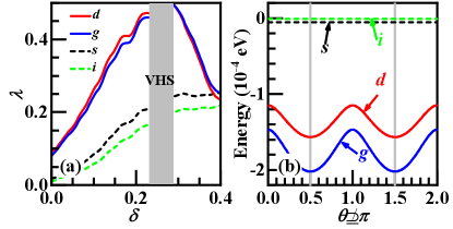
Figure 2(a) shows that the beneath-VH and beyond-VH doping regimes are covered by the degenerate $(d_{x^{2}-y^{2}},d_{xy})$- and $(g_{x^{4}-6x^{2}y^{2}+y^{4}},g_{x^{3}y-xy^{3}})$- doublets belonging to the 2D $E_{2}$- and $E_{4}$- IRRPs, respectively. The $s$-wave SC can emerge for $\delta>0.4$, and the other symmetries including the shown $i$-wave are always suppressed. The gap functions of these pairing states are provided in the SMSM . The two components of the $d$- or $g$-wave pairings are mixed as $1:\alpha e^{i\theta}$, and consequently the ground-state energies shown in Fig. 2(b) are minimized at $\alpha=1$ and $\theta=\pm\pi/2$SM , leading to the $d+id$- or $g+ig$- SCs, which can be well understood by the G-L theorySM .

Note that each possible ground-state gap function $\Delta(\mathbf{k})$ forms a 1D IRRP of the $C_{12}$ sub-groupSM : for each rotation by the angle $\Delta\phi=n\pi/6$, we have $\Delta(\mathbf{k})\to e^{-i\Delta\phi_{SC}}\Delta(\mathbf{k})=e^{-iL\Delta\phi}\Delta(\mathbf{k})$, with $L=0$ for the $s$ and $i*i^{\prime}$, $L=2$ for the $d+id$, $L=4$ for the $g+ig$ and $L=6$ for the $i$ and $i^{\prime}$. Fig. 2 suggests that the cases $L=2,4$ are realized in the QC-TBG. Interestingly, this result can be understood by the following G-L theory from the weak Josephson coupling between the previously obtained $d+id$ pairings in the two monolayers Doniach2007 ; Gonzalez2008 ; Honerkamp2008 ; Pathak2010 ; McChesney2010 ; Nandkishore2012 ; Wang2012 ; Kiesel2012 ; Honerkamp2014 .

Suppose the normalized gap form factors (either in the real or $\mathbf{k}$ space) on the t/b layers are $\Delta^{(\text{t/b})}_{d+id}$, we havefootnote2

Here $\hat{P}_{\phi}$ denotes the rotation by $\phi$. Setting the global “complex amplitudes” of the pairing gap functions on the t/b layers as $\psi_{\text{t/b}}$ footnote3 , the free energy function $F$ satisfying all the symmetries of QC-TBG reads (see the SMSM ),

Here the $F_{0}$- and the $A$- terms denote the contributions from each monolayer and their Josephson coupling respectively. The $A>0$ and $\theta\in(-\pi,\pi]$ are real numbers.

Now let’s rotate the system by $\Delta\phi=\frac{\pi}{6}$, followed by a succeeding layer exchange, under which Eq. (7) dictates

Here we use the convention with fixed $\Delta^{(\mu)}_{d+id}$. By symmetry, we have $F(\tilde{\psi_{\text{t}}},\tilde{\psi_{\text{b}}})=F(\psi_{\text{t}},\psi_{\text{b}})$, dictating

Under $A>0$, as the two layers are identical, $F$ should be minimized at $\psi_{\text{b}}=e^{i\theta}\psi_{\text{t}}$. The solution $\theta=\pi/3$ or $-2\pi/3$ makes $(\tilde{\psi_{\text{t}}},\tilde{\psi_{\text{b}}})=e^{-i\frac{\pi}{3}}(\psi_{\text{t}},\psi_{\text{b}})$ or $e^{i\frac{2\pi}{3}}(\psi_{\text{t}},\psi_{\text{b}})$, corresponding to $L=\frac{\pi}{3}/\Delta\phi=2$ or $\frac{-2\pi}{3}/\Delta\phi=-4$, respectively. Both solutions are supported by our microscopic calculations in different doping regimes.

More heuristically, our results can also be understood directly by the definition $L=\Delta\phi_{SC}/\Delta\phi$. As there is a $2n\pi$ uncertainty in $\Delta\phi_{SC}$, we should investigate the rotation by the minimum angle $\Delta\phi_{m}$. For each monolayer with $D_{6}$ symmetry, $\Delta\phi_{m}=\pi/3$. If we rotate the QC-TBG by $\pi/3$, then the $d+id$ pairing with $L=2$ within each mono-layer causes $\Delta\phi_{SC}=2\pi/3$ in that layer, as well as in the coupled system. This $\Delta\phi_{SC}$ can also be indistinguishably viewed as $-4\pi/3$. However, the emergent $D_{12}$ symmetry in the QC-TBG allows for the rotation by $\Delta\phi_{m}=\pi/6$, under which we have either $\Delta\phi_{SC}=\pi/3$ causing $L=2$, or $\Delta\phi_{SC}=-2\pi/3$ causing $L=-4$, which are distinguishable now. Our microscopic calculation results allow for both phases in different doping regimes.

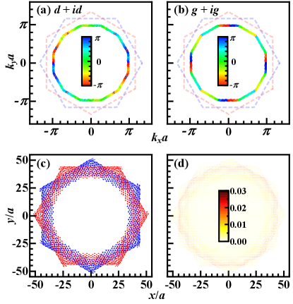
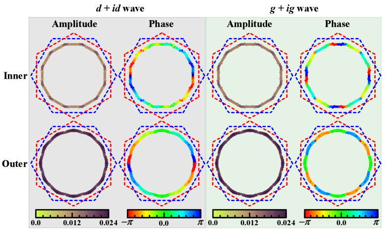
Novel TSC: The distributions of the gap amplitudes of the obtained $d+id$- and $g+ig$- SCs on the FSs are fully gappedSM , and those of their gap phases are shown in Figs. 3 (a) and (b) on the inner pocket for $\delta=0.32$ (those on the outer pocket are shown in the SMSM ). Clearly for each run around the pocket, the gap phases of the $d+id$- and $g+ig$- TSCs changes $4\pi$ and $8\pi$, leading to the winding numbers $2$ and $4$, and hence the Chern- numbers $C=2$ and $4$ per pocket respectivelySM .

The $g+ig$- TSC obtained here is novel, as it belongs to the 2D $E_{4}$- IRRP absent for the typical $D_{2n}$ point group on periodic lattices. Generally, the 2D IRRPs of $D_{2n}$ include the $E_{L}$ with $L\leq n-1$SM . For periodic lattices, we have $n\leq 3$ and hence $L\leq 2$, corresponding to the $p+ip$ and $d+id$. Here in the QC-TBG, we have $n=6$ and hence $L\leq 5$, including the $g+ig$. Although on periodic lattices with, say $D_{6}$ symmetry, the $g+ig$ can also emerge as a higher-harmonics basis function of the $E_{2}$- IRRP, it’s generally mixed with the $d+id$ as both belong to the $E_{2}$. Occasionally, the mixing weight of the $d+id$- component vanishes and one gets the $g+ig$Chichinadze2020 , which is accidental and rare. Here, the $g+ig$ TSC is protected by symmetry not to mix with the $d+id$ one.

The difference between the properties of the TSCs on extrinsic and intrinsic QCs is clarified here. It’s illustrated in Ref. Caoye2020 that on such intrinsic QC as the Penrose lattice, the lack of translational symmetry causes spontaneous bulk super current in chiral TSCs. However, as shown in Fig. 3(c) for the chiral $g+ig$ TSC obtained with open boundary condition, the super current only distributes at the edge with chiral pattern. As proved in the SMSM , the bulk current vanishes in the case of intra-band pairing between opposite momenta, caused by the nearly translational symmetry here. Similarly, the Majorana zero modesSM are also localized at the edge, as shown in Fig. 3(d). These properties make the TSCs on extrinsic QCs different from those on intrinsic QCs.

Conclusion and Discussions: In conclusion, we have revised the perturbational band theory to suit it for the study of e-e interaction driven SCs on extrinsic QCs. This $\mathbf{k}$-space approach is more convenient than the real-space onesLoring2016 ; Sakai2017 ; Andrade2019 ; Sakai2019 ; Nagai2020 ; Caoye2020 ; Sakai2020 ; YYZhang2020 to study the properties of the pairing states, as we can intuitively examine the distribution of the pairing gap functions on the FS. Consequently, this work for the QC-TBG reveals a novel $g+ig$ TSC with $L=4$ rare on periodic lattices, whose physical origin can be well understood from the G-L theory.

This approach also applies to other extrinsic QCs. One example is the 45°-twisted bilayer cuprate film. While Ref. cuprates_QC has studied the cases with commensurate twist angle $\theta$, the case of $\theta=45\degree$ can be studied by our approach. This approach can also be used to study other instabilities. One example is the spin density wave (SDW) in the VH-doped QC-TBG induced by the weak coupling between the chiral SDW ordersWang2012 ; Li2012 in the two mono-layers. Finally, since our approach is fully microscopic, we can use it to control electron phases through tuning such parameters as the inter-layer coupling or the displacement field, to achieve more exotic phases.

References

- (1) Y. Cao, V. Fatemi, A. Demir, S. Fang, S. L. Tomarken, J. Y. Luo, J. D. Sanchez-Yamagishi, K. Watanabe, T. Taniguchi, E. Kaxiras, R. C. Ashoori, and P. Jarillo-Herrero, Nature 556, 80 (2018).
- (2) Y. Cao, V. Fatemi, S. Fang, K. Watanabe, T. Taniguchi, E. Kaxiras, and P. Jarillo-Herrero, Nature 556, 43 (2018).
- (3) M. Yankowitz, S. Chen, H. Polshyn, Y. Zhang, K. Watanabe, T. Taniguchi, D. Graf, A. F. Young, and C. R. Dean, Science 363, 1059 (2019).
- (4) A. Kerelsky, L. J. McGilly, D. M. Kennes, L. Xian, M. Yankowitz, S. Chen, K. Watanabe, T. Taniguchi, J. Hone, C. Dean, A. Rubio, and A. N. Pasupathy, Nature 572, 95 (2019).
- (5) Y. Xie, B. Lian, B. Jäck, X. Liu, C.-L. Chiu, K. Watanabe, T. Taniguchi, B. A. Bernevig, and A. Yazdani, Nature 572,101 (2019).
- (6) X. Lu, P. Stepanov, W. Yang, M. Xie, M. A. Aamir, I. Das, C. Urgell, K. Watanabe, T. Taniguchi, G. Zhang, A. Bachtold, A. H. MacDonald, and D. K. Efetov, Nature 574, 653 (2019).
- (7) A. L. Sharpe, E. J. Fox, A. W. Barnard, J. Finney, K. Watanabe, T. Taniguchi, M. A. Kastner, D. Goldhaber-Gordon, Science 365, 605 (2019).
- (8) M. Serlin, C. L. Tschirhart, H. Polshyn, et al, Science 367,6480 (2019).
- (9) X. Liu, Z. Hao, E. Khalaf, J. Y. Lee, K. Watanabe, T. Taniguchi, A. Vishwanath, and P. Kim, Nature 583, 221 (2020).
- (10) A. Uri, S. Grover, Y. Cao, J. A. Crosse, K. Bagani, D. Rodan-Legrain, Y. Myasoedov, K. Watanabe, T. Taniguchi, P. Moon, M. Koshino, P. Jarillo-Herrero and E. Zeldov, Nature 581,47 (2020).
- (11) Z. Hao, A. M. Zimmerman, P. Ledwith, E. Khalaf, D. H. Najafabadi, K. Watanabe, T. Taniguchi, A. Vishwanath, and P. Kim, Science 371, 1133 (2021).
- (12) Y. Cao, D. Rodan-Legrain, J. M. Park, N. F. Yuan, K. Watanabe, T. Taniguchi, R. M. Fernandes, L. Fu, and P. Jarillo-Herrero, Science 372, 264 (2021).
- (13) C. Xu and L. Balents, Phys. Rev. Lett. 121, 087001 (2018).
- (14) H. C. Po, L. Zou, A. Vishwanath, and T. Senthil, Phys. Rev. X 8, 031089 (2018).
- (15) N. F. Q. Yuan and L. Fu, Phys. Rev. B 98, 045103 (2018).
- (16) C.-C. Liu, L.-D. Zhang, W.-Q. Chen, and F. Yang, Phys. Rev. Lett. 121, 217001 (2018).
- (17) F. Wu, A. H. MacDonald, and I. Martin, Phys. Rev. Lett. 121, 257001 (2018).
- (18) J. Kang and O. Vafek, Phys. Rev. X 8, 031088 (2018).
- (19) H. Isobe, N. F. Yuan, and L. Fu, Phys. Rev. X 8, 041041 (2018).
- (20) M. Koshino, N. F. Yuan, T. Koretsune, M. Ochi, K. Kuroki, and L. Fu, Phys. Rev. X 8, 031087 (2018).
- (21) J. W. Venderbos and R. M. Fernandes, Phys. Rev. B 98, 245103 (2018).
- (22) J. Kang and O. Vafek, Phys. Rev. Lett. 122, 246401 (2019).
- (23) H. C. Po, L. Zou, T. Senthil, and A. Vishwanath, Phys. Rev. B 99, 195455 (2019).
- (24) J. Liu, Z. Ma, J. Gao, and X. Dai, Phys. Rev. X 9, 031021 (2019).
- (25) L. Klebl and C. Honerkamp, Phys. Rev. B 100, 155145 (2019).
- (26) J. Gonzalez and T. Stauber, Phys. Rev. Lett. 122, 026801 (2019).
- (27) Z. Song, Z. Wang, W. Shi, G. Li, C. Fang, and B. A. Bernevig, Phys. Rev. Lett. 123, 036401 (2019).
- (28) J. Ahn, S. Park, and B.-J. Yang, Phys. Rev. X 9, 021013 (2019).
- (29) M. Angeli, E. Tosatti, and M. Fabrizio, Phys. Rev. X 9, 041010 (2019).
- (30) B. Lian, Z. Wang, and B. A. Bernevig, Phys. Rev. Lett. 122, 257002 (2019).
- (31) J. Liu, J. Liu, and Xi Dai, Phys. Rev. B 99, 155415 (2019).
- (32) G. Tarnopolsky, A. J. Kruchkov, and A. Vishwanath, Phys. Rev. Lett. 122, 106405 (2019).
- (33) Y.-P. Lin and R. M. Nandkishore, Phys. Rev. B 100, 085136 (2019); ibid, Phys. Rev. B 102, 245122 (2020).
- (34) Ming Xie, A. H. MacDonald, Phys. Rev. Lett. 124, 097601 (2020)
- (35) A. Abouelkomsan, Z. Liu, and E. J. Bergholtz, Phys. Rev. Lett. 124, 106803 (2020).
- (36) N. Bultinck, E. Khalaf, S. Liu, S. Chatterjee, A. Vishwanath, and M. P. Zaletel, Phys. Rev. X 10, 031034 (2020).
- (37) C. Repellin, Z. Dong, Y.-H. Zhang, and T. Senthil, Phys. Rev. Lett. 124, 187601 (2020).
- (38) Y. D. Liao, J. Kang, C. N. Brei, X. Y. Xu, H.-Q. Wu, B. M. Andersen, R. M. Fernandes, and Z. Y. Meng, Phys. Rev. X 11, 011014 (2021).
- (39) D. V. Chichinadze, L. Classen, and A. V. Chubukov, Phys. Rev. B 101, 224513 (2020).
- (40) M. Alidoust, A.-P. Jauho, and J. Akola, Phys. Rev. Res. 2, 032074(R) (2020).
- (41) X. Wu, W. Hanke, M. Fink, M. Klett and R. Thomale, Phys. Rev. B 101, 134517 (2020).
- (42) S. J. Ahn, P. Moon, T.-H. Kim, H.-W. Kim, H.-C. Shin, E. H. Kim, H. W. Cha, S.-J. Kahng, P. Kim, M. Koshino, Y.-W. Son, C.-W. Yang, J. R. Ahn, Science 361, 782 (2018).
- (43) W. Yao, E. Wang, C. Bao, Y. Zhang, K. Zhang, K. Bao, C. K. Chan, C. Chen, J. Avila, M. C. Asensio, J. Zhu, and S. Zhou, PNAS 115, 6928 (2018).
- (44) C. Yan, D.-L. Ma, J.-B. Qiao, H.-Y. Zhong, L. Yang, S.-Y. Li, Z.-Q. Fu, Y. Zhang and L. He, 2D Mater. 6, 045041 (2019).
- (45) S. Pezzini, V. Miseikis, G. Piccinini, S. Forti, S. Pace, R. Engelke, F. Rossella, K. Watanabe, T. Taniguchi, P. Kim and C. Coletti, Nano Lett. 20, 3313 (2020).
- (46) B. Deng, B. Wang, N. Li, R. Li, Y. Wang, J. Tang, Q. Fu, Z. Tian, P. Gao, J. Xue and H. Peng, ACS Nano 14, 1656 (2020).
- (47) P. Moon, M. Koshino, Phys. Rev. B 87, 205404 (2013).
- (48) M. Koshino, New J. Phys. 17, 015014 (2015).
- (49) P. Moon, M. Koshino, and Y.-W. Son, Phys. Rev. B 99, 165430 (2019).
- (50) M. J. Park, H. S. Kim and S. Lee, Phys. Rev. B 99, 245401(2019).
- (51) J. A. Crosse and Pilkyung Moon, Phys. Rev. B 103, 045408 (2021).
- (52) G. Yu, Z. Wu, Z. Zhan, M. I. Katsnelson and S. Yuan, npj Comput Mater 5, 122 (2019).
- (53) G. Yu, M. I. Katsnelson and S. Yuan, Phys. Rev. B 102, 045113 (2020).
- (54) G. Yu, Z. Wu, Z. Zhan, M. I. Katsnelson and S. Yuan, Phys. Rev. B 102, 115123 (2020).
- (55) J. L. Aragon, G. G. Naumis and A. Gomez-Rodriguez, Crystals 9, 519 (2019).
- (56) A. M. Black-Schaffer, and S. Doniach, Phys. Rev. B 75, 134512 (2007).
- (57) J. Gonzalez, Phys. Rev. B 78, 205431 (2008).
- (58) C. Honerkamp, Phys. Rev. Lett. 100, 146404 (2008).
- (59) S. Pathak, V. B. Shenoy, and G. Baskaran, Phys. Rev. B 81, 085431 (2010).
- (60) J. L. McChesney, A. Bostwick, T. Ohta, T. Seyller, K. Horn, J. Gonzalez, and E. Rotenberg, Phys. Rev. Lett. 104, 136803 (2010).
- (61) R. Nandkishore, L. S. Levitov, and A. V. Chubukov, Nat. Phys. 8, 158 (2012).
- (62) W.-S. Wang, Y.-Y. Xiang, Q.-H. Wang, F. Wang, F. Yang, and D.-H. Lee, Phys. Rev. B 85, 035414 (2012).
- (63) M. Kiesel, C. Platt, W. Hanke, D. A. Abanin, R. Thomale, Phys. Rev. B 86, 020507 (2012).
- (64) A. M. Black-Schaffer and C. Honerkamp, J. Phys. Condens. Matter 26, 423201 (2014).
- (65) P. Rosenzweig, H. Karakachian, D. Marchenko, K. Kuster, and U. Starke, Phys. Rev. Lett. 125, 176403 (2020).
- (66) W. DeGottardi, D. Sen, and S. Vishveshwara, Phys. Rev. Lett. 110, 146404 (2013).
- (67) X. Cai, L.-J. Lang, S. Chen, and Y. Wang, Phys. Rev. Lett. 110, 176403 (2013).
- (68) I. C. Fulga, D. I. Pikulin, and T. A. Loring, Phys. Rev. Lett. 116, 257002 (2016).
- (69) S. Sakai, N. Takemori, A. Koga, and R. Arita, Phys. Rev. B 95,024509 (2017).
- (70) R. N. Araújo and E. C. Andrade, Phys. Rev. B 100, 014510 (2019).
- (71) S. Sakai and R. Arita, Phys. Rev. Res. 1, 022002(R) (2019).
- (72) D. Varjas, A. Lau, K. Poyhonen, A. R. Akhmerov, D. I. Pikulin and I. C. Fulga, Phys. Rev. Lett. 123, 196401 (2019).
- (73) Y. Nagai, J. Phys. Soc. Jpn. 89, 074703 (2020).
- (74) Y. Cao, Y. Zhang, Y.-B. Liu, C.-C. Liu, W.-Q. Chen, and F. Yang, Phys. Rev. Lett. 125, 017002 (2020).
- (75) N. Takemori, R. Arita, and S. Sakai, Phys. Rev. B 102, 115108 (2020).
- (76) Y.-Y. Zhang, Y.-B. Liu, Y. Cao, W.-Q. Chen, and F. Yang, arXiv:2002.06485.
- (77) J. B. Hauck, C. Honerkamp, S. Achilles, and D. M. Kennes, Phys. Rev. Res. 3, 023180 (2021).
- (78) C.-B. Hua, Z.-R. Liu, T. Peng, R. Chen, D.-H. Xu and B. Zhou, arXiv:2107.01439.
- (79) K. Kamiya, T. Takeuchi, N. Kabeya, N. Wada, T. Ishimasa, A. Ochiai, K. Deguchi, K. Imura, and N. K. Sato, Nat. Commun. 9, 154 (2018).
- (80) See the Supplementary Material for the details of the band structure, the MF approach, the pairing-symmetry classification, more informatios on the obtained gap functions, the two Ginzburg-Landau theory based analysises, and the topological properties of the system.
- (81) R. Bistritzer and A. H. MacDonald, Proc. Natl. Acad. Sci. 108, 12233 (2011).
- (82) J. M. B. L. dos Santos, N. M. R. Peres, and A. H. Castro Neto, Phys. Rev. Lett. 99, 256802 (2007).
- (83) E. S. Morell, and L. E. F. Foa, Phys. Rev. B 86, 155449 (2012).
- (84) R. Bistritzer and A. H. MacDonald, Phys. Rev. B. 81, 245412 (2010).
- (85) A. H. C. Neto, F. Guinea, N. M. R. Peres, K. S. Novoselov, and A. K. Geim, Rev. Mod. Phys. 81, 109 (2009).
- (86) As the intra-layer hopping and interaction strengths are much stronger than the inter-layer ones, one can reasonably first let each two degenerate -wave pairings on one mono-layer mix as , and then consider their inter-layer coupling. Further more, we only consider the cases wherein the pairings from the two layers are both or , because otherwise the system cannot gain energy from the inter-layer Josephson coupling. See the SMSM .
- (87) The pairing gap functions on the t/b layers are written as , where are complex-valued “amplitudes”.
- (88) O. Can, T. Tummuru, R. P. Day, I. Elfimov, A. Damascelli, and M. Franz, Nat. Phys. 17, 519(2021).
- (89) T. Li, Europhys. Lett. 97, 37001 (2012).
I perturbational band theory
This section provides some details of the perturbational-band-theory approach adopted in our study for the free-electron part of the quasi-crystal twisted bilayer graphene (QC-TBG). We will provide here detailed information of the band structure, the Fermi surface (FS) and density of state (DOS) thus obtained for the system.
We start from the following tight-binding (TB) model of the QC-TBG,
- (1) P. Moon, M. Koshino and Y.-W. Son, Phys. Rev. B 99, 165430 (2019).
- (2) W. Yao, E. Wang, C. Bao, Y. Zhang, K. Zhang, K. Bao, C.-K. Chan, C. Chen, J. Avila, M. C. Asensio, J. Zhu and S. Zhou, PNAS 115, 6928 (2018).
- (3) M. Koshino, New J. Phys. 17, 015014 (2015).
- (4) S. Graser, T. A. Maier, P. J. Hirschfeld and D. J.Scalapino, New J. Phys. 11, 025016 (2009).
- (5) T. A. Maier, S. Graser, P. J. Hirschfeld and D. J. Scalapino, Phys. Rev. B 83, 100515(R) (2011).
- (6) W. Xu and X. Ka, "Group Theory and Application in Solid State Physics", Higher Education Press, Beijing (1999).
- (7) Y. Cao, Y. Zhang, Y.-B. Liu, C.-C. Liu, W.-Q. Chen and F. Yang, Phys. Rev. Lett. 125, 017002 (2020).
- (8) D. V. Chichinadze, L. Classen and A. V. Chubukov, Phys. Rev. B 101, 224513 (2020).
- (9) R. Nandkishore, L. S. Levitov and A. V. Chubukov, Nat. Phys. 8, 158 (2012).
- (10) X.-L. Qi, T. L. Hughes and S.-C. Zhang, Phys.Rev.B 82, 184516 (2010).
- (11) J. Alicea, Rep. Prog. Phys. 75, 076501 (2012).