Geometrizing quantum dynamics of a Bose-Einstein condensate

Geometries may arise as emergent phenomena in certain quantum systems. Prototypical examples include the AdS/CFT correspondence Maldacena (1999); Sachdev (2011), the ER$=$EPR conjecture Chapman et al. (2019); Jefferson and Myers (2017); Maldacena and Susskind (2013); Maldacena (2003), and scale invariant tensor networks Pastawski et al. (2015); Nozaki et al. (2012); Swingle (2012); Miyaji et al. (2015). In these examples, a prerequisite for the emergent hyperbolic geometries is the existence of strong correlations in quantum many-body systems. A question thus arises as to whether one could use weakly interacting systems, where gauge theory/gravity duality is unavailable at the moment, to reveal some intriguing geometries.

In this work, we show that quantum dynamics of weakly interacting bosons have deep roots in the hyperbolic geometry. Whereas such dynamics has been extensively studied Donley et al. (2001); Wu and Niu (2001); Nguyen et al. (2017); Hu et al. (2019); Bradley et al. (1995); Mun et al. (2007), our geometric approach has a number of unique advantages compared to the previous works. On the theoretical side, it leads to new understandings of prior experimental results. It shows that a fundamental concept of dynamical instability has an underlying geometric interpretation, corresponding to open trajectories on a Poincaré disk, a prototypical model for the hyperbolic surface. In sharp contrast, stable modes are mapped to closed trajectories, and the transition from stable to unstable mode can be visualized by the change of topology of the trajectories on the Poincaré disk.

In practice, our approach provides experimentalists with a powerful tool to access and manipulate new quantum dynamical phenomena. It delivers SU(1,1) echoes to reverse any initial state of any excitation mode once interactions of BECs change, as analogous to spin echoes overcoming the dephasing in spin systems Hahn (1950); Bluhm et al. (2010). Moreover, it could be used as a new framework to detect perturbations that breaks the SU(1,1) symmetry, in the same spirit of using spin echoes to extract a wide range of useful information when spins are interacting with each other Hahn and Maxwell (1952); Rowan et al. (1965); Liao and Hartmann (1973); Peng et al. (2015); Kinross et al. (2014). Finally, our scheme based on the SU(1,1) algebra and its underlying geometric representation applies to any systems with the SU(1,1) symmetry, similar to spin echoes broadly applied to systems whose constituents obey the SU(2) algebra. Our scheme thus can be used to reverse quantum dynamics in a wide range of systems and explore information scrambling via out-of-time ordering correlators (OTOC) Shenker and Stanford (2014); Maldacena et al. (2016); Li et al. (2017); Gärttner et al. (2017).

To be specific, this geometric approach correlates the time in quantum dynamics to the length in the hyperbolic space, and to the temperature that captures thermalization of a subsystem, as follows,

	$\displaystyle\tilde{L}=|\xi|t,$		(1)
	$\displaystyle\tilde{T}=-\frac{1}{2}\ln^{-1}\tanh(2\tilde{L}),$		(2)

where $\tilde{L}$ is the dimensionless length in a hyperbolic geometry and $\tilde{T}$ is the dimensionless temperature. $|\xi|$ is an energy scale characterizing the Hamiltonian and $t$ is the time. Each point on the Poincaré disk is assigned a unique SU(1,1) coherent state, and the overlap between two nearby SU(1,1) coherent states, which is denoted by $F_{z,z+dz}$, is equated to the metric of a Poincaré disk,

$$ds^{2}=4(1-F_{z,z+dz})=\frac{4(dx^{2}+dy^{2})}{(1-x^{2}-y^{2})^{2}},$$

(3)

where $(x,y)$ denote Cartesian coordinates.

We consider a Hamiltonian

$$H=\sum_{\vec{k}}E_{\vec{k}}c_{\vec{k}}^{\dagger}c_{\vec{k}}+\frac{\tilde{U}}{2V}\sum_{\vec{k},\vec{k^{\prime}},\vec{q}}c_{\vec{k}+\vec{q}}^{\dagger}c_{\vec{k^{\prime}}-\vec{q}}^{\dagger}c_{\vec{k^{\prime}}}c_{\vec{k}},$$

(4)

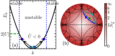
where $\tilde{U}=4\pi\hbar^{2}\frac{a_{s}}{M}$, $c^{\dagger}_{\vec{k}}$ ($c_{\vec{k}}$) is the creation (annihilation) operator for bosons with the momentum ${\vec{k}}$. Starting from $t=0$, $a_{s}(t)$ is tuned dynamically from either zero or a small value using the magnetic or optical Feshbach resonance Chin et al. (2010), as shown in Fig. 1. Our results based on the SU(1,1) algebra apply to both quenching $a_{s}$ or an arbitrary $a_{s}(t)$ sup .

Though a BEC with attractive interactions is not stable Donley et al. (2001); Bradley et al. (1995); Mun et al. (2007), coherent dynamics is achievable within a timescale before significant losses of particles occur Chen and Hung (2019). We first focus on short-time dynamics in which the particle number at a finite momentum, $N_{\vec{k}\neq 0}$, is small such that interactions among excitations are negligible. The quantum dynamics is governed by a Hamiltonian, $H_{\text{eff}}=\sum_{\vec{k}}H_{\vec{k}}$,

$$H_{\vec{k}}(t)=\xi_{0}({\vec{k}})K_{0}+\xi_{1}({\vec{k}})K_{1}+\xi_{2}({\vec{k}})K_{2},$$

(5)

where $K_{0}=\frac{1}{2}(c_{\vec{k}}^{\dagger}c_{\vec{k}}+c_{-\vec{k}}c_{-\vec{k}}^{\dagger})$, $K_{1}=\frac{1}{2}(c_{\vec{k}}^{\dagger}c_{-\vec{k}}^{\dagger}+c_{\vec{k}}c_{-\vec{k}})$ and $K_{2}=\frac{1}{2i}(c_{\vec{k}}^{\dagger}c_{-\vec{k}}^{\dagger}-c_{\vec{k}}c_{-\vec{k}})$, $\xi_{0}(\vec{k})=2(E_{\vec{k}}+\tilde{U}|\Psi_{0}|^{2})$, $\xi_{1}(\vec{k})=2\real U$, $\xi_{2}(\vec{k})=-2\imaginary U$, $U=\tilde{U}\Psi_{0}^{2}$, and $\Psi_{0}=\sqrt{{N_{0}}/{V}}e^{i\theta}$ is the condensate wavefunction. $\vec{\xi}=\{\xi_{0},\xi_{1},\xi_{2}\}$ is an external field, analogous to the magnetic field in the case of SU(2), and its strength, $\xi=\sqrt{\xi_{0}^{2}-\xi_{1}^{2}-\xi_{2}^{2}}$, characterizes the energy scale. For instance, when $\xi_{0}^{2}>\xi_{1}^{2}+\xi_{2}^{2}$, the energy spectrum is given by $(m+1/2)\xi$, where $m$ is an integer. The above equations show that the dynamics at different ${\vec{k}}$ are decoupled. This model can be realized using a wide range of apparatuses sup .

The Hamiltonian in Eq. (5) with arbitrary choices of parameters, $\xi_{1,2,3}$, can be generated by three operators, $K_{0}$, $K_{1}$ and $K_{2}$, which satisfy

$$[K_{1},K_{2}]=-iK_{0},\ [K_{0},K_{1}]=iK_{2},\ [K_{2},K_{0}]=iK_{1}.$$

(6)

Any propagator,

$$P(t)={\text{T}}e^{-i\int_{0}^{t}dt^{\prime}H_{\vec{k}}(t^{\prime})},$$

(7)

is an element in SU(1,1) Novaes (2004), where T is the time-ordering operator. Such SU(1,1) symmetry was recently revisited and a special type of echo applicable to an initial state of the vacuum in periodically driven bosons was discussed Chen et al. (2020); Chih and Holland (2020). Since the global $U(1)$ phase does not affect physical observables, we consider the quotient, $SU(1,1)/U(1)$, whose element is created by two operations,

$\displaystyle R(\varphi_{0})=e^{-i\varphi_{0}K_{0}},\,\,\,\,\,B(\varphi_{1},0)=e^{-i\varphi_{1}K_{1}},$

(8)

which correspond to a rotation and a boost, respectively. A generic boost along an arbitrary direction is given by $B(\varphi_{1},\varphi_{2})=e^{-i(\varphi_{1}K_{1}+\varphi_{2}K_{2})}$.

Eq. (8) provides us with a parametrization of the propagators using a Poincaré disk Gilmore (2008); Novaes (2004), as shown in Fig. 1(b). A similar approach was revisited very recently to consider geometric phases in the adiabatic limit Cheng and Shi (2020). Whereas both the SU(1,1) symmetry of the Hamiltonian and the geometric representation of $SU(1,1)/U(1)$ are known in the literature Novaes (2004); Gilmore (2008); Novaes (2004), many fundamental questions remain unexplored. For instance, whether the metric of the Poincaré disk defined geometrically has any correspondence to physical quantities of the quantum system? Does a geodesic, the shortest distance between two points, leads to any significant observations in quantum dynamics? We will answer these questions in the following discussions.

To establish a one-to-one correspondence between the quantum dynamics and a Poincaré disk, we consider the vacuum, $|\Psi(0)\rangle=|0\rangle_{\vec{k}}|0\rangle_{-\vec{k}}$, where $c_{\vec{k}}|0\rangle_{\vec{k}}=0$. The two operators in Eq. (8) deliver a wavefunction, $|z\rangle=R(\varphi_{0})B(\varphi_{1},0)R^{\dagger}(\varphi_{0})\ket{\Psi(0)}$, which is written as

$\displaystyle\begin{aligned} |z\rangle=\sqrt{1-|z|^{2}}\sum_{n}z^{n}\ket{n}_{\vec{k}}\ket{n}_{-\vec{k}},\end{aligned}$

(9)

where $z=-ie^{-i\varphi_{0}}\tanh\frac{\varphi_{1}}{2}$ and $\ket{n}_{\vec{k}}=c^{\dagger n}_{{\vec{k}}}|0\rangle/\sqrt{n!}$. In high energy physics, the expression in Eq. (9) is called a thermofield double state (TFD) state Chapman et al. (2019); Jefferson and Myers (2017); Maldacena and Susskind (2013); Maldacena (2003); Maldacena et al. (2016); Shenker and Stanford (2014). In quantum optics, it is referred to as a two-mode squeezed state, which can be created through non-degenerate parametric amplification Scully and Zubairy (1997). Creating squeezed states from squeeze operators has been well studied in quantum optics Gerry (1991), and such a connection with BECs has also been recently studied Chih and Holland (2020). Eq. (9) can be derived using explicit forms of the boost and rotation operators sup . Since $|z|=|x+iy|\leq 1$, we identify each TFD in Eq. (9) with a unique point on the Poincaré disk.

Tracing over half of the system in TFD leaves the other half with a thermal density matrix,

$$\rho_{\vec{k}}=\Tr_{-\vec{k}}\ket{z}\bra{z}=\mathcal{Z}^{-1}\sum_{n}e^{-\frac{nE_{{\vec{k}}}}{k_{B}{T}}}\ket{n}_{\vec{k}}\bra{n}_{\vec{k}},$$

(10)

similar to Hawking radiation and Unruh effects Hawking (1974); Unruh (1976). In Eq. (10), we have identified the Euclidean distance to the center of the disk, $|z|$, with a temperature,

$$\tilde{T}\equiv\frac{k_{B}T}{E_{k}}=-\frac{1}{2}\ln^{-1}|z|,$$

(11)

and $\mathcal{Z}=1-e^{-{E_{\vec{k}}}/{{k_{B}T}}}$. Each point on the Poincaré disk can be assigned with a temperature and the boundary circle corresponds to $T=\infty$. In quantum information, the closeness between two states is often characterized by their overlap, i.e., their fidelity Wilde (2013). Here, the fidelity between TFDs, $F_{z,z^{\prime}}=|\langle z^{\prime}|z\rangle|^{2}$, is written as,

$$|\langle z|z^{\prime}\rangle|^{2}=\frac{(1-|z|^{2})(1-|z^{\prime}|^{2})}{|1-z^{*}z^{\prime}|^{2}}.$$

(12)

Consider two TFDs close to each other on the Poincaré disk, i.e., $z^{\prime}=z+dz$, from the above expression, we obtain Eq. (3). The fidelity between TFDs thus corresponds to the metric of a Poincaré disk. The metric of a Poincaré disk can also be correlated to the complexities of the SU(1,1) coherent states Chapman et al. (2018).

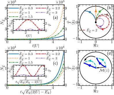
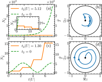
We now consider quenching $a_{s}(t)$ from zero to a finite negative value. When $E_{\vec{k}}>2|U|$ or equivalently, $\xi^{2}>0$, the growth of $n_{\vec{k}}$ is bounded from above and is referred as to a stable mode. On the Poincaré disk, it is described by a closed loop, as shown in Fig. 2(b). When $E_{\vec{k}}=2|U|$, $\xi$ vanishes and the topology of the trajectory changes. When $E_{\vec{k}}<2|U|$, i.e., $\xi^{2}<0$, the well-known dynamical instability occurs and $n_{\vec{k}}$ grows exponentially, mimicking the inflation in the early universe Hu et al. (2019). On the Poincaré disk, any unstable mode corresponds to an open trajectory, starting from the origin and extending to the circular boundary. However, it takes infinite time to reach there, since the boundary of the Poincaré disk corresponds to infinity.

When $E_{\bf k}=|U|$, starting from the center of the Poincaré disk, the trajectory follows the diameter, i.e., a geodesic. The Euclidean distance to the center is written as

$\displaystyle|z(t)|=\Bigg{\{}\begin{array}[]{ll}\left(1-\frac{\xi^{2}}{\xi_{1}^{2}+\xi_{2}^{2}}\frac{1}{\sinh^{2}(\frac{|\xi|t}{2})}\right)^{-\frac{1}{2}},&\xi^{2}<0\\ \left(1+\frac{\xi^{2}}{\xi_{1}^{2}+\xi_{2}^{2}}\frac{1}{\sin^{2}(\frac{|\xi|t}{2})}\right)^{-\frac{1}{2}},&\xi^{2}>0.\end{array}$

(15)

We see from Eq. (15) that, if we fix ${\xi_{1}^{2}+\xi_{2}^{2}}$, $|z(t)|$ grows fastest when $\xi_{0}=0$, i.e., when the system moves along the geodesic. Under this situation,

$$|z(t)|_{g}=\tanh(\frac{|\xi|}{2}t).$$

(16)

Using the metric in Eq. (3), the length along the geodesic is given by

$$\tilde{L}=\int_{0}^{|z(t)|_{g}}\frac{2dx}{1-x^{2}}={|\xi|}t.$$

(17)

We thus have proved Eq. (1). Using Eq. (11), Eq. (16) and Eq. (17), it is also straightforward to prove Eq. (2). It is worth pointing out that, once $|\xi|$ is fixed, Eq. (15) shows that the geodesic corresponds to the slowest growth among unstable modes. As seen from numerical results plotted in Fig. 2(c), the resonant mode does grow slower than other unstable modes. For off-resonant modes, the trajectories are no longer geodesics and the length along such a trajectory as a function of the time has an expression similar to Eq. (17) (Supplemental Materials).

If the initial scattering length is finite, the ground state is no longer a vacuum. The quantum dynamics starts from a point away from the center of the Poincaré disk. A Möbius transformation preserving the metric, $z^{\prime}=\mathcal{M}(z)=\frac{\alpha z+\beta}{\beta^{*}z+\alpha^{*}}$, $\quad|\alpha|^{2}-|\beta|^{2}=1$, could map the origin to any other point on the disk, and thus all phenomena remain the same compared with starting from a vacuum. For any initial and final states, $|z_{1}\rangle$ and $|z_{2}\rangle$, the quantum dynamics could follow a geodesic, which in general is not a straight line, using a Hamiltonian,

$\displaystyle\begin{aligned} H/|\xi|=&\frac{-\imaginary z_{1}z_{2}^{*}}{|z_{1}-z_{2}||z_{1}z_{2}^{*}-1|}(c_{\vec{k}}^{\dagger}c_{\vec{k}}+c_{-\vec{k}}c_{-\vec{k}}^{\dagger})\\ +&\frac{i(z_{2}-z_{1}+|z_{1}|^{2}z_{2}-|z_{2}|^{2}z_{1})}{2|z_{1}-z_{2}||z_{1}z_{2}^{*}-1|}c_{\vec{k}}^{\dagger}c_{-\vec{k}}^{\dagger}+\text{h.c.}.\end{aligned}$

(18)

To realize the Hamiltonian in Eq. (18), it is required that one could tune $\theta$ in Eq. (5) sup .

We now turn to periodic drivings. Consider an example that is directly relevant to current experiments,

	$\displaystyle H_{1}$	$\displaystyle=2(E_{\vec{k}}+U)K_{0}+2UK_{1},$	$\displaystyle 0<t<t_{1}$		(19)
	$\displaystyle H_{2}$	$\displaystyle=2E_{\vec{k}}K_{0},$	$\displaystyle t_{1}<t<T_{d},$		(20)

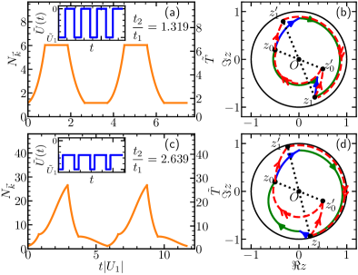
where the period $T_{d}=t_{1}+t_{2}$. It corresponds to periodically modifying the interaction strength in Eq. (4). When $a_{s}=0$, the propagator from $t=t_{1}$ to $t=T_{d}$ is given by Eq. (8), i.e., a rotation about the center of the Poincaré disk. Such drivings allow us to manipulate both the stable and unstable modes sup . A particularly interesting case is a quantum revival of the initial state at the end of the second period. We emphasize that such a revival is accessible for any initial state, and any $H_{1}$ in Eq. (19), not requiring a vacuum as the initial state nor a Hamiltonian satisfying the resonant condition Hu et al. (2019); Chen et al. (2020). We consider an arbitrary $H_{1}=w_{0}K_{0}+w_{1}K_{1}+w_{2}K_{2}$ with a field strength $w$. The Baker-Hausdorff-Campbell formula decomposes the propagator $\mathcal{U}_{1}=e^{-iH_{1}t_{1}}$ into

$$\mathcal{U}_{1}=e^{-i\zeta_{1}K_{0}}e^{-i\eta_{1}(K_{1}\cos\phi_{1}+K_{2}\sin\phi_{1})}e^{-i\zeta_{1}K_{0}},$$

(21)

where $\zeta_{1}=\arctan(\frac{w_{0}}{w}\tan\frac{wt_{1}}{2})$, $\phi_{1}=\arccos(\frac{w_{1}}{\sqrt{w_{1}^{2}+w_{2}^{2}}})$, and $\eta_{1}=2\operatorname{arcsinh}\left(\frac{\sqrt{w_{1}^{2}+w_{2}^{2}}}{w}\sin(\frac{wt_{1}}{2})\right)$.

A quantum revival on a Poincaré disk requires that $(\mathcal{U}_{2}\mathcal{U}_{1})^{2}=1$. Using the identity $B(\eta\cos\phi,\eta\sin\phi)R(\pi)B(\eta\cos\phi,\eta\sin\phi)=R(\pi)$, where $\phi$ and $\eta$ are two arbitrary real numbers, we conclude that $\mathcal{U}_{2}=e^{-iH_{2}t_{2}}$ should satisfy

$$\mathcal{U}_{2}=e^{-i\pi K_{0}}e^{-i(K_{1}\cos\phi+K_{2}\sin\phi)\eta}\mathcal{U}_{1}^{-1}.$$

(22)

This SU(1,1) echo is analogous to the standard spin echo using SU(2) Hahn (1950), and is applicable in a variety of bosonic systems. $\mathcal{U}_{2}\mathcal{U}_{1}$ corresponds to an arbitrary boost followed by a $\pi$-rotation, $\mathcal{U}_{2}\mathcal{U}_{1}=R(\pi)B(\eta\cos\phi,\eta\sin\phi)$. Eq. (22) readily determines $H_{2}$ and $t_{2}$. Since $\phi$ and $\eta$ are arbitrary, for any $H_{1}$, there is a family of $H_{2}$, not just a single Hamiltonian, that could lead to the revival.

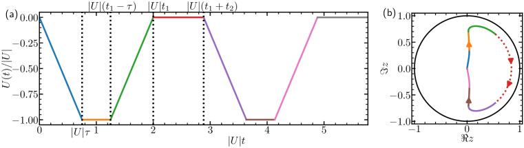
Choosing $\eta=\eta_{1},\quad\phi=\phi_{1}-\zeta_{1}$, we obtain $H_{2}=u_{0}K_{0}$, and $t_{2}=(\pi-2\zeta_{1})/u_{0}$. This means that quenching back to zero scattering length in Eq. (5) during the time interval from $t_{1}$ to $t_{2}$ reverses the quantum dynamics at $t=2(t_{1}+t_{2})$, as shown in Fig. 3. Alternatively, if we quench the scattering length to a finite value, which amounts to a different choice of $\eta$ and $\phi$, the trajectory from $t=t_{1}$ to $t=t_{2}$ is no longer a concentric circle on the Poincaré disk. Nevertheless, an appropriate $t_{2}$ still leads to a quantum revival, as shown in Fig. 3. If we define $B(\eta\cos\phi,\eta\sin\phi)|z_{0}\rangle=|z_{1}^{\prime}\rangle$, $B(\eta\cos\phi,\eta\sin\phi)|z_{1}\rangle=|z_{0}^{\prime}\rangle$, we see that $z_{0}=-z_{0}^{\prime}$ and $z_{1}=-z_{1}^{\prime}$ are satisfied by both cases, providing us with a geometric interpretation of the quantum revival. We thus conclude, for any $H_{1}$ and $t_{1}$, there is a family of $H_{2}$ to deliver $e^{-iH_{2}t_{2}}e^{-iH_{1}t_{1}}e^{-iH_{2}t_{2}}=e^{iH_{1}t_{1}}$. The SU(1,1) echo thus effectively creates a reversed evolution based on $-H_{1}$, an essential ingredient in studying OTOC Shenker and Stanford (2014); Maldacena et al. (2016); Li et al. (2017); Gärttner et al. (2017).

We now consider interactions between excited particles. As the population of the resonant mode grows fastest when $U$ is fixed, interactions at this mode become the dominant corrections. The Hamiltonian becomes $\tilde{H}_{\vec{k}}=H_{\vec{k}}+H_{\vec{k}}^{\prime}$, where $H_{\vec{k}}^{\prime}=U^{\prime}(4c_{\vec{k}}^{\dagger}c_{\vec{k}}c_{-\vec{k}}^{\dagger}c_{-\vec{k}}+c_{\vec{k}}^{\dagger}c_{\vec{k}}^{\dagger}c_{\vec{k}}c_{\vec{k}}+c_{-\vec{k}}^{\dagger}c_{-\vec{k}}^{\dagger}c_{-\vec{k}}c_{-\vec{k}})$ can be rewritten as

$$H_{\vec{k}}^{\prime}=6U^{\prime}(K_{0}-2/3)^{2},$$

(23)

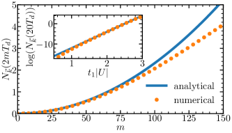
if the initial state is the two-mode vacuum. Without loss of generality, we have denoted the interactions between excited particles as $U^{\prime}$. Here, $U^{\prime}=\tilde{U}/2V$ but in other systems, $U^{\prime}$ might be independent of the unperturbed Hamiltonian. A finite $U^{\prime}$ breaks the SU(1,1) symmetry, and an SU(1,1) echo will not lead to a perfect revival of the initial state. The SU(1,1) echo thus can be implemented as a unique tool to measure the interactions between excited particles, in the same spirit of using the spin echo to extract interactions between spins and other useful information. Using the SU(1,1) algebra, we obtain analytical results of the population at $t=2mT_{d},m\in\mathbb{N}$ sup ,

$\displaystyle N_{\vec{k}}(2mT_{d})=\frac{27\cosh(8\tilde{U}|\Psi_{0}|^{2}t_{1})}{16\tilde{U}^{2}|\Psi_{0}|^{4}}m^{2}U^{{}^{\prime}2}.$

(24)

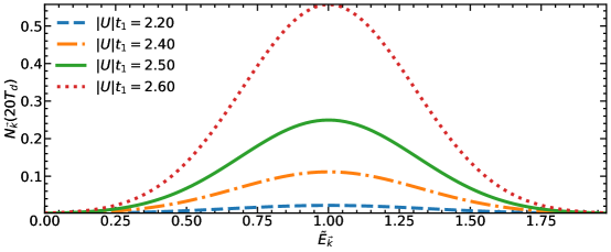
Confirmed by numerical calculations, Eq. (24) shows that $N_{\vec{k}}(2mT_{d})$ vanishes when $U^{\prime}=0$. If $U^{\prime}\neq 0$, $N_{\vec{k}}(2mT_{d})$ increases quadratically as a function of $m$, as shown in Fig.(4). Thus, the imperfect revival unveils $U^{\prime}$. In particular, $N_{\vec{k}}(2mT_{d})$ depends on $\tilde{U}|\Psi_{0}|^{2}t_{1}$ exponentially. Increasing $t_{1}$ could further improve the precision of the measurement. Alternatively, if $U^{\prime}$ is known, Eq. (24) allows experimentalists to measure $\tilde{U}|\Psi_{0}|^{2}t_{1}$ with high precision due to the exponential dependence of $N_{\vec{k}}(2mT_{d})$ on this parameter.

Whereas we have been focusing on quenching and periodically driving interactions in BECs, our results obtained by algebraic methods apply to any systems with the SU(1,1) symmetry, including but not limited to the unitary fermions and 2D bosons and fermions with contact interaction Werner and Castin (2006); Deng et al. (2016); Son (2007); Elliott et al. (2014); Gerry (1989). For instance, SU(1,1) echoes could be implemented to breathers of two-dimensional BECs, which was recently studied in an elegant experiment Saint-Jalm et al. (2019). We hope that our work will stimulate more research efforts to unfold the intrinsic entanglement between dynamics, algebras, and geometries.

This work is supported by DOE DE-SC0019202, W. M. Keck Foundation, and a seed grant from PQSEI.

Supplementary Materials for “Geometrizing quantum dynamics of a Bose-Einstein condensate”

Modulating the scattering length

The magnetic Feshbach resonance is a standard technique to deliver a time-dependent scattering length, $a_{s}(t)$. For instance, the experiment done at Chicago used BEC of ¹³³Cs atoms in the hyperfine state $\ket{F=3,m_{F}=3}$ Hu et al. (2019). An external magnetic field was modulated around 17.22G such that the scattering length oscillates in a fashion of $a_{dc}+a_{ac}\sin\omega t$, where $\omega$ is the modulation frequency of the magnetic field, $a_{dc}$ is the stationary part of $a_{s}$ and $a_{ac}$ denotes the amplitude of the oscillation.

In reality, it takes a a finite time to change the magnetic field unlike the optical Feshbach resonance that could easily give rise to an abrupt change in $a_{s}$. It is, therefore, desired to consider a generic time-dependence of $a_{s}$ in addition to the quench dynamics. For any time-dependent Hamiltonian, $H(t)=2(E_{\vec{k}}+U(t))K_{0}+2U(t)K_{1}$, where $U(t)=4\pi\hbar^{2}\frac{a_{s}(t)}{M}\Psi_{0}^{2}$. For an arbitrary $U(t)$, the propagator $\text{T}e^{\int_{0}^{t_{1}}-iH(t^{\prime})dt^{\prime}}$ , where T is the time-ordering operator, is still an element in the SU(1,1) group. It thus can be rewritten as $\exp(-iH_{\rm eff}t_{1})$, where $H_{\rm eff}=w_{0}K_{0}+w_{1}K_{1}+w_{2}K_{2}$ is time-independent. Whereas the exact expressions of $w_{0,1,2}$ depend on the explicit form of $U(t)$, $\exp(-iH_{\rm eff}t_{1})$ can always be decomposed to a boost and a rotation, as discussed in the main text. Therefore the SU(1,1) echoes still apply.

To demonstrate the SU(1,1) echoes for a generic $U(t)$, we consider linearly turning on and off the scattering length $a_{s}$. The time dependent $U(t)$ is shown in Fig.5. The $H_{\rm eff}$ and the corresponding $t_{2}$ required for the SU(1,1) echo is obtained numerically. The trajectory on the Poincaré disk is also shown.

Alternatively, the optical Feshbach resonance could be implemented so as to change the scattering length fast enough compared to other time scales relevant to many-body physics such as the interaction strength Yamazaki et al. (2010); Nicholson et al. (2015) A quench dynamics can then be realized.

SU(1,1) coherent state

Here, we supply the derivation of Eq.(9) in the main text. The boost operator $B(\varphi_{1},0)=\exp(-i\varphi_{1}K_{1})$ can be written in its normal ordering form Puri (2001)

$$\exp(-i\varphi_{1}K_{1})=\exp(-i\tanh(\frac{\varphi_{1}}{2})K_{+})\exp(-2\ln(\cosh(\frac{\varphi_{1}}{2}))K_{0})\exp(-i\tanh(\frac{\varphi_{1}}{2})K_{-}),$$

(25)

where $K_{\pm}=K_{1}\pm iK_{2}$. We note that

$$K_{0}\ket{n}_{\vec{k}}\ket{n}_{-\vec{k}}=\left(n+\frac{1}{2}\right)\ket{0}_{\vec{k}}\ket{0}_{-\vec{k}},\quad K_{-}\ket{0}_{\vec{k}}\ket{0}_{-\vec{k}}=0,\quad K_{+}^{n}\ket{0}_{\vec{k}}\ket{0}_{-\vec{k}}=n!\ket{n}_{\vec{k}}\ket{n}_{-\vec{k}},$$

(26)

and apply $R(\varphi_{0})B(\varphi_{1},0)R^{\dagger}(\varphi_{0})=\exp(-i\varphi_{0}K_{0})\exp(-i\varphi_{1}K_{1})\exp(i\varphi_{0}K_{0})$ to $\ket{\Psi(0)}=\ket{0}_{\vec{k}}\ket{0}_{-\vec{k}}$, and obtain

$$\begin{split}R(\varphi_{0})B(\varphi_{1},0)R^{\dagger}(\varphi_{0})\ket{\Psi(0)}=&\sum_{n=0}^{\infty}e^{-i\varphi_{0}(n+1/2)}\left(-i\tanh(\frac{\varphi_{1}}{2})\right)^{n}\cosh^{-1}\left(\frac{\varphi_{1}}{2}\right)e^{i\varphi_{0}/2}\ket{n}_{\vec{k}}\ket{n}_{-\vec{k}}\\ =&\sqrt{1-|z|^{2}}\sum_{n=0}^{\infty}z^{n}\ket{n}_{\vec{k}}\ket{n}_{-\vec{k}},\end{split}$$

(27)

where $z=-ie^{-i\varphi_{0}}\tanh(\frac{\varphi_{1}}{2})$.

Lengths of trajectories

We consider the quench dynamics where the initial state is the vacuum. The state at time $t$ is

$$\ket{z(t)}=e^{-i(\xi_{0}K_{0}+\xi_{1}K_{1}+\xi_{2}K_{2})t}\ket{0}_{\vec{k}}\ket{0}_{-\vec{k}}=\mathcal{U}(t)\ket{0}_{\vec{k}}\ket{0}_{-\vec{k}}.$$

(28)

$z(t)$ can be evaluated by writing $\mathcal{U}(t)$ in its normal ordering form Puri (2001), and we will have

$$z(t)=-i\frac{(\xi_{1}-i\xi_{2})\sin(\xi t/2)}{\xi\cos(\xi t/2)+i\xi_{0}\sin(\xi t/2)},\ \xi=\sqrt{\xi_{0}^{2}-\xi_{1}^{2}-\xi_{2}^{2}}.$$

(29)

Therefore, the length of the trajectory as a function of $t$ on the Poincaré disk is

$$\tilde{L}=\int_{0}^{t}\sqrt{4\left|\frac{dz}{dt^{\prime}}\right|^{2}\frac{1}{(1-|z(t^{\prime})|^{2})^{2}}}dt^{\prime}=|\xi_{1}-i\xi_{2}|t,$$

(30)

which holds for any $\xi_{0,1,2}\in\mathbb{R}$. Eq. (30) reduces to $|\xi|t$ when we consider the resonance mode, where $\xi_{0}=0$, $|\xi|=|\xi_{1}-i\xi_{2}|$, which is Eq. (15) in the main text.

Realizations of the model

There are multiple means to realize the model in Eq.(4) of the main text.

I. Shaken lattices

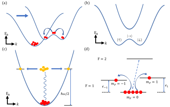
In shaken lattices, the single-particle energy can be tuned by hybridizing different bands. In particular, one could create a double-well structure in the momentum space Parker et al. (2013). Therefore, starting from a conventional band structure where a condensate occupies the zero momentum state, suddenly changing the band structure to a double-well one, a pair of particles can be scattered from a condensate to states with opposite momenta. The resultant dynamics become similar to the ones discussed in the main text.

II. Spin-orbit coupling

A double-well structure in the momentum space can also be created using spin-orbit coupling, as the single-particle dispersions of spin-up and spin-down atoms move towards opposite directions in the $k$-space Galitski and Spielman (2013). Moreover, the interaction strength also becomes momentum dependent, as the eigenstate is a momentum-dependent superposition of spin-up and spin-down Li et al. (2019). This provides experimentalists with a new degree of freedom to tune parameters in the model in Eq.(4) of the main text.

III. Periodic driving

Periodically modifying the scattering length could resonantly couple the condensate at zero momentum to a pair of states with opposite momenta. In the rotating wave approximation, the model is the same as the one discussed in the main text. This scheme was implemented in an experiment done at Chicago Hu et al. (2019). A theoretically work has also studied corrections beyond the rotating wave approximation and used the SU(1,1) algebra in the calculations to discuss a revival scheme similar to ours Chen et al. (2020). However, the geometrization to hyperbolic surface was not discussed. Near the completion of our manuscript, another theoretical work discussed the parameterization to the hyperbolic surface but the metric was not explored Cheng and Shi (2020). Therefore, geodesics and their physical meanings, as well as schemes of coherently controlling the dynamics, eluded this work.

IV. Spinor condensates

In spinor condensate, there is a well-known spin-mixing term in the Hamiltonian, $a^{\dagger 2}_{0}a_{1}a_{-1}+h.c$, where $a_{m=0,\pm 1}$ are the creation operators at $m_{F}=0,\pm 1$ states in the $F=1$ manifold Ho (1998); Law et al. (1998). This term precisely corresponds to $K_{1}$ and $K_{2}$ in the model discussed in the main text. Using a combination of the magnetic field and the couplings to $F=2$ manifold, the energy of the three hyperfine spin states are also tunable such that we have $(\epsilon_{1}+\epsilon_{-1})(a^{\dagger}_{1}a_{1}+a^{\dagger}_{-1}a_{-1})/2$ in the HamiltonianLuo et al. (2017). Prepare the initial state as a condensate occupying $m_{F}=0$, density-density interactions can be ignored in the timescale where the population at $m_{F}=\pm 1$ is much smaller than that at $m_{F}=0$. The model becomes identical to ours. We point out that, the linear Zeeman splitting, $(\epsilon_{1}-\epsilon_{-1})(a^{\dagger}_{1}a_{1}-a^{\dagger}_{-1}a_{-1})/2$, commutes with our Hamiltonian and has no effect on the dynamics.

V. Two-mode squeezing in optics

In non-linear medium inside a resonant cavity, the pump beam undergoes spontaneous parametric down-conversion (SPDC) and generates entangled photon pairs, which couples resonant modes and causes two-mode squeezing. The coupling term is controlled by the external pump fieldScully and Zubairy (1997). Starting from the two-modes vacuum and turning on the pump field, the dynamics is captured by Eq.(4) of the main text.

Whereas interactions between atoms in the excited states of BECs modify the TFD by adding additional relative phases between $k$ and $-k$, such interaction effects are absent in two-mode squeezing in quantum optics, since the interactions between photons are absent. The Hamiltonian is the same as Eq. (5) in the main text Scully and Zubairy (1997); Puri (2001); Yurke et al. (1986), where $a^{\dagger}_{k}a^{\dagger}_{-k}+h.c.$ is replaced by the corresponding operators of photons, $a^{\dagger}b^{\dagger}+h.c.$. It thus delivers an authentic TFD.

Changing the phase of $U$

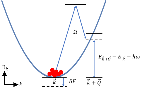
As for the realization discussed in the main text, since $U=\frac{4\pi\hbar a_{s}}{M}\Psi_{0}^{2}$, adding a phase to $\Psi_{0}$ could change the phase of $U$. This can be achieved using a pulse of Bragg scattering, as shown in Fig. 7. The Bragg beams couple a momentum state $|{\vec{k}}\rangle$ to another one $|\vec{k}+\vec{Q}\rangle$. When the transition is off-resonance, the Bragg coupling leads to a shift of the energy of $|{\vec{k}}\rangle$,

$$\delta E_{\vec{k}}=-\frac{\Omega^{2}}{\Delta_{\vec{k}}}=-\frac{\Omega^{2}}{E_{\vec{k}+\vec{Q}}-E_{\vec{k}}-\hbar\omega},$$

(31)

where $\Omega$ is the coupling strength of Bragg scattering, $\omega$ and $\vec{Q}$ are the differences in the frequency and momentum of these two beams. Therefore, such a pulse provides $|{\bf k}\rangle$ a phase shift $e^{-i\delta\varphi_{\vec{k}}}=e^{-i\delta E_{\vec{k}}\tau}$, where $\tau$ is the duration of the pulse.

For fixed $\vec{Q}$ and $\omega$, $\delta E_{\vec{k}}$ is a linear function of $\vec{k}$. Therefore, the condensate at zero momentum acquires a different phase compared to state at a finite momentum ${\bf k}$ that we are interested in. Effectively, we have added an phase $\phi=2\delta\varphi_{0}-\delta\varphi_{\vec{k}}-\delta\varphi_{-\vec{k}}$ to the Hamiltonian in Eq.(4) of the main text. This method is also applicable to realizations (I-III) discussed in the previous section.

As for spinor condensate, this scheme can be even simpler as we have discrete hyperfine spin states other than the continuum in the momentum space. We could selectively couple $|1,0\rangle$ to a state in the $F=2$ manifold, such as $|2,0\rangle$, as shown in Fig. 6(d). The other two hyperfine spin states are not affected or weakly coupled. Then the phase of $U$ is also controllable. As for two-mode squeezing, $U$ corresponds to an external field and its phase can be easily controlled.

Controllable dynamics using periodic drivings

Consider the periodic driving in the main text,

	$\displaystyle H_{1}$	$\displaystyle=2(E_{\vec{k}}+U)K_{0}+2UK_{1},$	$\displaystyle 0<t<t_{1}$		(32)
	$\displaystyle H_{2}$	$\displaystyle=2E_{\vec{k}}K_{0},$	$\displaystyle t_{1}<t<T_{d},$		(33)

where the period $T_{d}=t_{1}+t_{2}$. When $a_{s}=0$, the propagator from $t=t_{1}$ to $t=T_{d}$ is a rotation about the center of the Poincaré disk. Though during this time interval, $N_{\vec{k}}$ and $\tilde{T}$ remain unchanged, starting from $t=T_{d}$, the dynamics becomes drastically different when the interaction is turned on again. Depending on where the trajectory ends at $t=T_{d}$, the growth of $N_{{\vec{k}}}$ and $\tilde{T}$ in the second period can be faster or slower than the first period for both the stable and unstable modes. For instance, for a stable mode, in a single quench dynamics, $N_{\vec{k}}$ is always bounded from above. In contrast, a periodic driving can systematically move the system to circles further and further away from the center, and even the stable mode could reach any desired $N_{\vec{k}}$. We have verified this phenomenon from numerical calculations as shown in Fig. 8(c, d). The growth of $N_{\vec{k}}$ and $\tilde{T}$ can also be slowed down, provided that the trajectory in the second period moves towards the center of the Poincaré disk. For instance, the inflation in an unstable mode can be significantly slowed down, as shown in Fig. 8(a, b).

The increase of the particle number when the SU(1,1) symmetry is broken

In this section, we provide the derivation of Eq.(22) in the main text. The Floquet Hamiltonians in the presence of the interaction term $(K_{0}-2/3)^{2}$ for the resonance mode is written as

	$\displaystyle H^{\prime}_{1}$	$\displaystyle=2UK_{1}+6U^{\prime}(K_{0}-2/3)^{2},$	$\displaystyle mT_{d}<t<mT_{d}+t_{1}$		(34)
	$\displaystyle H_{2}$	$\displaystyle=-2UK_{0},$	$\displaystyle mT_{d}+t_{1}<t<(m+1)T_{d}.$		(35)

We have chosen $t_{2}=\pi/(-2U)$ such that an echo delivers a perfect revival if $U^{\prime}=0$. There is no $U^{\prime}$ term during $mT_{d}+t_{1}<t<(m+1)T_{d}$ since here we consider $U^{\prime}=\tilde{U}/2V$, and during this time period the interaction is off. The propagator from $t=0$ to $t=t_{1}$ can be written as

$$\mathcal{U}^{\prime}_{1}=e^{-i(2UK_{1}+6U^{\prime}((K_{0}-2/3))^{2})t_{1}}=e^{-i2UK_{1}t_{1}}e^{-i\int_{0}^{t_{1}}6U^{\prime}(K_{0}(t)-2/3)^{2}dt+O(U^{{}^{\prime}2})},\quad K_{0}(t)=e^{i2UK_{1}t}K_{0}e^{-i2UK_{1}t},$$

(36)

where we have used the Dyson series up to the first order of $U^{\prime}$. Therefore, we have

$$\mathcal{U}(2T_{d})=\mathcal{U}_{2}\mathcal{U}^{\prime}_{1}\mathcal{U}_{2}\mathcal{U}^{\prime}_{1}=e^{i\pi}e^{-i\int_{0}^{t_{1}}12U^{\prime}(K_{0}(t)-2/3)^{2}dt},$$

(37)

and

$$\begin{split}N_{\vec{k}}(2mT_{d})=&\langle 0|\mathcal{U}(-2mT_{d})\left(K_{0}-\frac{1}{2}\right)\mathcal{U}(2mT_{d})|0\rangle\\ =&\langle 0|K_{0}-\frac{m^{2}}{2}\left[\int_{0}^{t_{1}}12U^{\prime}(K_{0}(t)-2/3)^{2}dt,\left[\int_{0}^{t_{1}}12U^{\prime}(K_{0}(t)-2/3)^{2}dt,K_{0}\right]\right]+O(U^{{}^{\prime}3})|0\rangle-\frac{1}{2}\\ =&\frac{9m^{2}U^{{}^{\prime}2}}{16U^{2}}\left[3\cosh(8Ut_{1})-\frac{16}{3}\cosh(6Ut_{1})-16Ut_{1}\sinh(4Ut_{1})-8\cosh(4Ut_{1})\right.\\ &\left.+\frac{32}{3}\cosh(4Ut_{1})+\frac{16}{3}\cosh(2Ut_{1})+32(Ut_{1})^{2}-\frac{17}{3}\right]+O(U^{{}^{\prime}3})\\ \approx&\frac{27}{16}\frac{m^{2}U^{{}^{\prime}2}}{U^{2}}\cosh(8Ut_{1}),\end{split}$$

(38)

In the last step, we have dropped the $O(U^{{}^{\prime}3})$ term and made use of $\cosh(2Ut_{1})\gg 1$, since we are interested in a long enough time, $t_{1}$, so as to enhance the signal of $U^{\prime}$ in the echoes. For a generic $t_{1}$, other terms in the above equation should be also included.

References

- Maldacena (1999) J. Maldacena, The large-N limit of superconformal field theories and supergravity, International Journal of Theoretical Physics 38, 1113 (1999).
- Sachdev (2011) S. Sachdev, From Gravity to Thermal Gauge Theories: The AdS/CFT Correspondence (Springer Berlin Heidelberg, 2011) pp. 273–311.
- Chapman et al. (2019) S. Chapman, J. Eisert, L. Hackl, M. P. Heller, R. Jefferson, H. Marrochio, and R. C. Myers, Complexity and entanglement for thermofield double states, SciPost Physics 6 (2019).
- Jefferson and Myers (2017) R. A. Jefferson and R. C. Myers, Circuit complexity in quantum field theory, Journal of High Energy Physics 10, 107 (2017).
- Maldacena and Susskind (2013) J. Maldacena and L. Susskind, Cool horizons for entangled black holes, Fortschritte der Physik 61, 781 (2013).
- Maldacena (2003) J. Maldacena, Eternal black holes in anti-de sitter, Journal of High Energy Physics 04, 021 (2003).
- Pastawski et al. (2015) F. Pastawski, B. Yoshida, D. Harlow, and J. Preskill, Holographic quantum error-correcting codes: toy models for the bulk/boundary correspondence, Journal of High Energy Physics 06, 149 (2015).
- Nozaki et al. (2012) M. Nozaki, S. Ryu, and T. Takayanagi, Holographic geometry of entanglement renormalization in quantum field theories, Journal of High Energy Physics 10, 193 (2012).
- Swingle (2012) B. Swingle, Entanglement renormalization and holography, Phys. Rev. D 86, 065007 (2012).
- Miyaji et al. (2015) M. Miyaji, T. Numasawa, N. Shiba, T. Takayanagi, and K. Watanabe, Continuous multiscale entanglement renormalization ansatz as holographic surface-state correspondence, Phys. Rev. Lett. 115, 171602 (2015).
- Donley et al. (2001) E. A. Donley, N. R. Claussen, S. L. Cornish, J. L. Roberts, E. A. Cornell, and C. E. Wieman, Dynamics of collapsing and exploding Bose–Einstein condensates, Nature 412, 295 (2001).
- Wu and Niu (2001) B. Wu and Q. Niu, Landau and dynamical instabilities of the superflow of Bose-Einstein condensates in optical lattices, Phys. Rev. A 64, 061603 (2001).
- Nguyen et al. (2017) J. H. V. Nguyen, D. Luo, and R. G. Hulet, Formation of matter-wave soliton trains by modulational instability, Science 356, 422 (2017).
- Hu et al. (2019) J. Hu, L. Feng, Z. Zhang, and C. Chin, Quantum simulation of Unruh radiation, Nature Physics 15, 785 (2019).
- Bradley et al. (1995) C. C. Bradley, C. A. Sackett, J. J. Tollett, and R. G. Hulet, Evidence of Bose-Einstein condensation in an atomic gas with attractive interactions, Phys. Rev. Lett. 75, 1687 (1995).
- Mun et al. (2007) J. Mun, P. Medley, G. K. Campbell, L. G. Marcassa, D. E. Pritchard, and W. Ketterle, Phase diagram for a Bose-Einstein condensate moving in an optical lattice, Phys. Rev. Lett. 99, 150604 (2007).
- Hahn (1950) E. L. Hahn, Spin echoes, Phys. Rev. 80, 580 (1950).
- Bluhm et al. (2010) H. Bluhm, S. Foletti, I. Neder, M. Rudner, D. Mahalu, V. Umansky, and A. Yacoby, Dephasing time of GaAs electron-spin qubits coupled to a nuclear bath exceeding 200 s, Nature Physics 7, 109 (2010).
- Hahn and Maxwell (1952) E. L. Hahn and D. E. Maxwell, Spin echo measurements of nuclear spin coupling in molecules, Phys. Rev. 88, 1070 (1952).
- Rowan et al. (1965) L. G. Rowan, E. L. Hahn, and W. B. Mims, Electron-spin-echo envelope modulation, Phys. Rev. 137, A61 (1965).
- Liao and Hartmann (1973) P. F. Liao and S. R. Hartmann, Determination of cr-al hyperfine and electric quadrupole interaction parameters in ruby using spin-echo electron-nuclear double resonance, Phys. Rev. B 8, 69 (1973).
- Peng et al. (2015) X. Peng, H. Zhou, B.-B. Wei, J. Cui, J. Du, and R.-B. Liu, Experimental observation of lee-yang zeros, Phys. Rev. Lett. 114, 010601 (2015).
- Kinross et al. (2014) A. W. Kinross, M. Fu, T. J. Munsie, H. A. Dabkowska, G. M. Luke, S. Sachdev, and T. Imai, Evolution of quantum fluctuations near the quantum critical point of the transverse field ising chain system , Phys. Rev. X 4, 031008 (2014).
- Shenker and Stanford (2014) S. H. Shenker and D. Stanford, Black holes and the butterfly effect, Journal of High Energy Physics 03, 67 (2014).
- Maldacena et al. (2016) J. Maldacena, S. H. Shenker, and D. Stanford, A bound on chaos, Journal of High Energy Physics 08, 106 (2016).
- Li et al. (2017) J. Li, R. Fan, H. Wang, B. Ye, B. Zeng, H. Zhai, X. Peng, and J. Du, Measuring out-of-time-order correlators on a nuclear magnetic resonance quantum simulator, Phys. Rev. X 7, 031011 (2017).
- Gärttner et al. (2017) M. Gärttner, J. G. Bohnet, A. Safavi-Naini, M. L. Wall, J. J. Bollinger, and A. M. Rey, Measuring out-of-time-order correlations and multiple quantum spectra in a trapped-ion quantum magnet, Nature Physics 13, 781 (2017).
- Chin et al. (2010) C. Chin, R. Grimm, P. Julienne, and E. Tiesinga, Feshbach resonances in ultracold gases, Rev. Mod. Phys. 82, 1225 (2010).
- (29) See Supplemental Materials, which includes Refs. Yamazaki et al. (2010); Nicholson et al. (2015); Puri (2001); Parker et al. (2013); Galitski and Spielman (2013); Li et al. (2019); Ho (1998); Law et al. (1998); Luo et al. (2017); Yurke et al. (1986), for further discussions on the experimental realization, SU(1,1) coherent states, controllable dynamics using periodic drivings, lengths of trajectories, and the increase of the particle number when the SU(1,1) symmetry is broken.
- Chen and Hung (2019) C.-A. Chen and C.-L. Hung, Observation of modulational instability and Townes soliton formation in two-dimensional Bose gases (2019), arXiv:1907.12550 .
- Novaes (2004) M. Novaes, Some basics of su(1, 1), Revista Brasileira de Ensino de Física 26, 351 (2004).
- Chen et al. (2020) Y.-Y. Chen, P. Zhang, W. Zheng, Z. Wu, and H. Zhai, Many-body echo, Phys. Rev. A 102, 011301 (2020).
- Chih and Holland (2020) L.-Y. Chih and M. Holland, Driving quantum correlated atom-pairs from a bose–einstein condensate, New J. Phys. 22, 033010 (2020).
- Gilmore (2008) R. Gilmore, Lie Groups, Physics, and Geometry: An Introduction for Physicists, Engineers and Chemists (Cambridge University Press, 2008).
- Cheng and Shi (2020) Y. Cheng and Z.-Y. Shi, Many-body dynamics with time-dependent interaction (2020), arXiv:2004.12754 .
- Scully and Zubairy (1997) M. O. Scully and M. S. Zubairy, Quantum optics (Cambridge University Press, 1997).
- Gerry (1991) C. C. Gerry, Correlated two-mode SU(1, 1) coherent states: nonclassical properties, Journal of the Optical Society of America B 8, 685 (1991).
- Hawking (1974) S. W. Hawking, Black hole explosions?, Nature 248, 30 (1974).
- Unruh (1976) W. G. Unruh, Notes on black-hole evaporation, Phys. Rev. D 14, 870 (1976).
- Wilde (2013) M. M. Wilde, Quantum information theory (Cambridge University Press, 2013).
- Chapman et al. (2018) S. Chapman, M. P. Heller, H. Marrochio, and F. Pastawski, Toward a definition of complexity for quantum field theory states, Phys. Rev. Lett. 120, 121602 (2018).
- Werner and Castin (2006) F. Werner and Y. Castin, Unitary gas in an isotropic harmonic trap: Symmetry properties and applications, Phys. Rev. A 74, 053604 (2006).
- Deng et al. (2016) S. Deng, Z.-Y. Shi, P. Diao, Q. Yu, H. Zhai, R. Qi, and H. Wu, Observation of the efimovian expansion in scale-invariant fermi gases, Science 353, 371 (2016).
- Son (2007) D. T. Son, Vanishing bulk viscosities and conformal invariance of the unitary fermi gas, Phys. Rev. Lett. 98, 020604 (2007).
- Elliott et al. (2014) E. Elliott, J. A. Joseph, and J. E. Thomas, Observation of conformal symmetry breaking and scale invariance in expanding fermi gases, Phys. Rev. Lett. 112, 040405 (2014).
- Gerry (1989) C. C. Gerry, Berry’s phase in the degenerate parametric amplifier, Phys. Rev. A 39, 3204 (1989).
- Saint-Jalm et al. (2019) R. Saint-Jalm, P. C. M. Castilho, É. Le Cerf, B. Bakkali-Hassani, J.-L. Ville, S. Nascimbene, J. Beugnon, and J. Dalibard, Dynamical symmetry and breathers in a two-dimensional bose gas, Phys. Rev. X 9, 021035 (2019).
- Yamazaki et al. (2010) R. Yamazaki, S. Taie, S. Sugawa, and Y. Takahashi, Submicron spatial modulation of an interatomic interaction in a bose-einstein condensate, Phys. Rev. Lett. 105, 050405 (2010).
- Nicholson et al. (2015) T. L. Nicholson, S. Blatt, B. J. Bloom, J. R. Williams, J. W. Thomsen, J. Ye, and P. S. Julienne, Optical feshbach resonances: Field-dressed theory and comparison with experiments, Phys. Rev. A 92, 022709 (2015).
- Puri (2001) R. R. Puri, Mathematical methods of quantum optics (Springer, 2001).
- Parker et al. (2013) C. V. Parker, L.-C. Ha, and C. Chin, Direct observation of effective ferromagnetic domains of cold atoms in a shaken optical lattice, Nature Physics 9, 769 (2013).
- Galitski and Spielman (2013) V. Galitski and I. B. Spielman, Spin–orbit coupling in quantum gases, Nature 494, 49 (2013).
- Li et al. (2019) C.-H. Li, C. Qu, R. J. Niffenegger, S.-J. Wang, M. He, D. B. Blasing, A. J. Olson, C. H. Greene, Y. Lyanda-Geller, Q. Zhou, C. Zhang, and Y. P. Chen, Spin current generation and relaxation in a quenched spin-orbit-coupled bose-einstein condensate, Nature Communications 10 (2019).
- Ho (1998) T.-L. Ho, Spinor Bose condensates in optical traps, Phys. Rev. Lett. 81, 742 (1998).
- Law et al. (1998) C. K. Law, H. Pu, and N. P. Bigelow, Quantum spins mixing in spinor bose-einstein condensates, Phys. Rev. Lett. 81, 5257 (1998).
- Luo et al. (2017) X.-Y. Luo, Y.-Q. Zou, L.-N. Wu, Q. Liu, M.-F. Han, M. K. Tey, and L. You, Deterministic entanglement generation from driving through quantum phase transitions, Science 355, 620 (2017).
- Yurke et al. (1986) B. Yurke, S. L. McCall, and J. R. Klauder, SU(2) and SU(1,1) interferometers, Phys. Rev. A 33, 4033 (1986).