Geometric Static Modeling Framework for Piecewise-Continuous Curved-Link Multi Point-of-Contact Tensegrity Robots

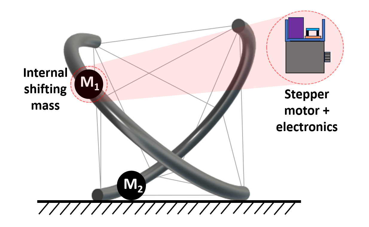
The Tensegrity eXploratory Robot (TeXploR), Fig. 1, comprises of two curved-links held together with a tensile cable with two motor assemblies that are free to move along the links. The two links, $\{L_{1},L_{2}\}$, are modeled as semi-circular arcs with radii $r$ with masses $\{m_{1},m_{2}\}$, Fig. 2. The two endpoints of the two arcs are denoted as $\{A_{i},B_{i}\}$ for link $L_{i}$. For the remainder of this section, $i=1,2$ corresponding to the two links. The body coordinate system $\{b\}$ is fixed on the robot body with origin $O_{b}$ and orthonormal basis $U_{b}=\left[\bm{x}_{b},\bm{y}_{b},\bm{z}_{b}\right]\in SO(3)$. Let coordinate systems $\{1,2\}$ be fixed on the corresponding link with origin at the center of each arc, such that the $x$ and $z$ axes respectively are along the arc end points $B_{i}A_{i}$, and normal to the arc plane. The center of the two links are coincident and $\{1\}$ coincides with $\{b\}$. The inertial coordinate system $\{s\}$ is fixed at origin $O_{s}$ with orthonormal basis $U_{s}=\left[\bm{x}_{s},\bm{y}_{s},\bm{z}_{s}\right]\in SO(3)$ such that $\bm{z}_{s}$ is normal to the plane of locomotion.

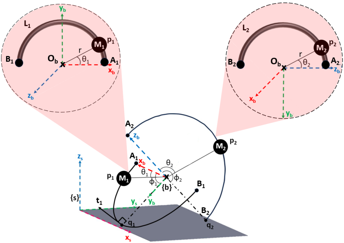
The motor assemblies are modeled as point masses $M_{i}$ that move along the corresponding link. These point masses $P_{i}$ are defined using angle $\theta_{i}$ from $\bm{x}_{i}$ and denoted by $\bm{p}_{i}\in\mathbb{R}^{3\times 1}$. The instantaneous points of contact, $Q_{i}$, between the links and the ground plane are represented by $\bm{q}_{i}\in\mathbb{R}^{3\times 1}$ and parameterized using ground contact angles $\phi_{i}$ from $\bm{x}_{i}$. The tangents of the arc at these instantaneous points of contact are denoted by $\bm{t}_{i}\in\mathbb{R}^{3\times 1}$. Terminology of the shifting masses and points of contact is summarized in Tab. I.

Ultimately, it is desired to find the transformation matrix $T_{sb}\in SE(3)$, such that

$\displaystyle T_{sb}=\begin{bmatrix}R_{sb}&\bm{o}_{sb}\\ \bm{0}_{3\times 1}&1\end{bmatrix}$

(1)

where $R_{sb}\in SO(3)$, $\bm{o}_{sb}$ are the rotation matrix and displacement between origins of $\{s\},\{b\}$.

The position vectors $\bm{p}_{i},\bm{q}_{i}$ are represented as a combination of the arc radius and respective angles along arcs.

$$\bm{p}_{i}^{i}=r\begin{bmatrix}c_{\theta_{i}}\\ s_{\theta_{i}}\\ 0\end{bmatrix},\quad\bm{q}_{i}^{i}=r\begin{bmatrix}c_{\phi_{i}}\\ s_{\phi_{i}}\\ 0\end{bmatrix}$$

(2)

where $c_{\alpha_{i}}=\cos(\alpha_{i}),s_{\alpha_{i}}=\sin(\alpha_{i}),\forall i=1,2,\alpha=\theta,\phi$, and the superscript $i$ refers to the c.s. of representation. The transformation matrix $T_{12}\in{SE}(3)$ changes the representation between c.s. $\{2\}$ to $\{1\}$. That is, for some vector $\bm{v}\in\mathbb{R}^{3\times 1}$

$\displaystyle\begin{gathered}\begin{bmatrix}\bm{v}^{1}\\ 1\end{bmatrix}=T_{12}\begin{bmatrix}\bm{v}^{2}\\ 1\end{bmatrix}\Rightarrow\bm{v}^{1}=\bm{o}_{12}^{1}+R_{12}\bm{v}^{2}\\ T_{12}=\begin{bmatrix}R_{12}&\bm{o}_{12}\\ \bm{0}_{1\times 3}&1\end{bmatrix},R_{12}=\begin{bmatrix}0&0&1\\ 0&-1&0\\ 1&0&0\\ \end{bmatrix},\bm{o}_{12}^{1}=\begin{bmatrix}0\\ 0\\ 0\end{bmatrix}\end{gathered}$

(5)

where $R_{12}\in SO(3)$ and $\bm{o}_{12}\in\mathbb{R}^{3\times 1}$ are the rotation matrix and the displacement between the origins of the $\{1\},\{2\}$. For the remainder of the paper, we disregard the superscript for the vector notation, as all the representations will be in the robot body c.s. $\{b\}$ which coincides with $\{1\}$. Hence,

$$\begin{gathered}\bm{p}_{1}=r\begin{bmatrix}c_{\theta_{1}}\\ s_{\theta_{1}}\\ 0\end{bmatrix},\quad\bm{p}_{2}=\bm{o}_{12}+R_{12}\bm{p}_{2}^{2}=r\begin{bmatrix}0\\ -s_{\theta_{2}}\\ c_{\theta_{2}}\end{bmatrix}\\ \bm{q}_{1}=r\begin{bmatrix}c_{\phi_{1}}\\ s_{\phi_{1}}\\ 0\end{bmatrix},\quad\bm{q}_{2}=\bm{o}_{12}+R_{12}\bm{q}_{2}^{2}=r\begin{bmatrix}0\\ -s_{\phi_{2}}\\ c_{\phi_{2}}\end{bmatrix}\end{gathered}$$

(6)

The ‘free-vector’ tangent $\bm{t}_{i}$ at points of contact $Q_{i}$ are

$\displaystyle\bm{t}_{i}=\frac{\partial\bm{q}_{i}}{\partial\phi_{i}}$

(7)

Pure rolling without slipping is assumed at the points of contact, $Q_{1},Q_{2}$. Hence, they have zero velocity, i.e., $\bm{\dot{q}}_{1}=\bm{\dot{q}}_{2}=0$. We use the Lie group approach for modeling and follow the notation as per[20]. The body twist, $\xi_{b}\in\mathbb{R}^{6}$, encodes the angular velocity $\omega_{b}$ and linear velocity of the origin $O_{b}$, $v_{b}$ expressed in $\{b\}$. The hat operator $~{}\hat{}~{}$ maps $\mathbb{R}^{6\times 1}\rightarrow\mathfrak{se}(3)$ and $\mathbb{R}^{3\times 1}\rightarrow\mathfrak{so}(3)$

$$\xi_{b}=\begin{bmatrix}\omega_{b}\\ v_{b}\end{bmatrix},\quad\widehat{\xi}_{b}=\begin{bmatrix}\widehat{\omega}_{b}&v_{b}\\ 0&0\end{bmatrix}\in\mathfrak{se}(3)$$

Following this notation, the rolling constraint is

$$\bm{\dot{q}}_{i}=v_{b}+\hat{\omega}_{b}\bm{q}_{i}=0$$

In this paper, we restrict ourselves to static analysis and do not examine this constraint given the modeling complexity, especially, the hybrid nature of such two-point contact system to be discussed next.

It is assumed that the robot is in physical contact with the surface of locomotion at all times. This implies that the two points $Q_{1},Q_{2}$ are in contact with the ground and the tangents at those points also lie on the ground plane. The ground plane is defined using the surface normal which is the z-axis $\bm{z}_{s}$ of $\{s\}$. Another kinematic interpretation of this is that the $\bm{z_{s}}$ component of position $\bm{q_{i}}$ is the minimum amongst all the points on the link. For the two points of contact $Q_{i}$

$\displaystyle\begin{gathered}[\bm{z_{s}}^{T},1]\cdot\left(T_{sb}\begin{bmatrix}\bm{q}_{i}\\ 1\end{bmatrix}\right)=0,\quad[\bm{z_{s}}^{T},1]\cdot\left(T_{sb}\begin{bmatrix}\bm{t}_{i}\\ 0\end{bmatrix}\right)=0\end{gathered}$

(9)

This can be simplified to

$\displaystyle\begin{gathered}\begin{bmatrix}(\bm{q}_{1}-\bm{q}_{2})^{T}\\ \left(\bm{t}_{1}\right)^{T}\\ \left(\bm{t}_{2}\right)^{T}\end{bmatrix}\bm{z_{b}}=\bm{0},\quad\bm{z_{b}}=R_{sb}^{T}\bm{z_{s}},~{}\mathrm{s.t.}\quad\bm{z}_{s}=\begin{bmatrix}0\\ 0\\ 1\end{bmatrix}\end{gathered}$

(11)

Geometrically, this implies that vectors $(\bm{q}_{1}-\bm{q}_{2}),\bm{t}_{1},\bm{t}_{2}$ lie in the same plane and the vector $\bm{z_{b}}$ is the surface normal. However, there is discontinuity at the edges of the links, i.e., $\phi_{i}=0,180\degree$ where the tangents cannot be defined. These discontinuities can be separated into three unique cases:

Case 1: Tangent vector $\bm{t}_{2}$ not defined. Here, vector $\bm{z}_{b}$ is normal to the vector $Q_{1}Q_{2}$ and tangent vector at $Q_{1}$. The direction of $\bm{z}_{b}$ can be deduced from the fact that $\bm{o}_{sb}$, origin $O_{b}$ of $\{b\}$ lies above the ground plane, i.e., $\bm{z}_{s}^{T}\bm{o}_{sb}>0$, and $Q_{1},Q_{2}$ are in contact with the ground. Mathematically,

$\displaystyle\bm{z}_{s}^{T}\left(\bm{o}_{sb}+R_{sb}\bm{q}_{i}\right)=0,~{}\mathrm{and}~{}\bm{z}_{s}^{T}\bm{o}_{sb}>0~{}\Rightarrow~{}-(\underbrace{R_{sb}^{T}\bm{z}_{s}}_{\bm{z}_{b}^{T}})^{T}\bm{q}_{i}>0$

The analytical solution for $\bm{z}_{b}$ can then be summarized as

$\displaystyle\begin{gathered}\bm{\bm{z}_{b}}=\pm\frac{\bm{t}_{1}\times(\bm{q}_{1}-\bm{q}_{2})}{|\bm{t}_{1}\times(\bm{q}_{1}-\bm{q}_{2})|}\quad\mathrm{s.t.}\quad-\bm{z}_{b}^{T}\bm{q}_{1}=-\bm{z}_{b}^{T}\bm{q}_{2}>0\\ \bm{\bm{z}_{b}}=-\frac{1}{\sqrt{2}}[c_{\phi_{1}},s_{\phi_{1}},c_{\phi_{2}}]^{T},\quad-\bm{z}_{b}^{T}\bm{q}_{1}=-\bm{z}_{b}^{T}\bm{q}_{2}=\frac{r}{\sqrt{2}}\end{gathered}$

(14)

Case 2: Tangent vector $\bm{t}_{1}$ not defined. Similar to the previous case, $\bm{z}_{b}$ is normal to the vector $Q_{1}Q_{2}$ and the tangent vector at $Q_{2}$. Using the surface-contact constraint, the analytical expression of unique $\bm{z}_{b}$ is

$\displaystyle\begin{gathered}\bm{\bm{z}_{b}}=\pm\frac{\bm{t}_{2}\times(\bm{q}_{2}-\bm{q}_{1})}{|\bm{t}_{2}\times(\bm{q}_{2}-\bm{q}_{1})|}\quad\mathrm{s.t.}\quad-\bm{z}_{b}^{T}\bm{q}_{1}=-\bm{z}_{b}^{T}\bm{q}_{2}>0\\ \bm{\bm{z}_{b}}=\frac{1}{\sqrt{2}}[-c_{\phi_{1}},s_{\phi_{2}},-c_{\phi_{2}}]^{T},\quad-\bm{z}_{b}^{T}\bm{q}_{1}=-\bm{z}_{b}^{T}\bm{q}_{2}=\frac{r}{\sqrt{2}}\end{gathered}$

(17)

Given that the surface normal is defined only for cases 1 and 2, the robot can be modeled as a hybrid system transitioning between four states. Each case corresponds to the robot instantaneously pivoting about about one of the end points of the curved link.

1. State 1: $\phi_{1}\in(0,180\degree),\phi_{2}=\phantom{1}0\degree,\phantom{8}$ $A_{2}$ pivot, roll along $L_{1}$

2. State 2: $\phi_{1}\in(0,180\degree),\phi_{2}=180\degree$, $B_{2}$ pivot, roll along $L_{1}$

3. State 3: $\phi_{1}=\phantom{1}0\degree\phantom{8},\phi_{2}\in(0,180\degree)$, $A_{1}$ pivot, roll along $L_{2}$

4. State 4: $\phi_{1}=180\degree,\phi_{2}\in(0,180\degree)$, $B_{1}$ pivot, roll along $L_{2}$

As an example, the geometric representation of the robot in State 2 and pivoting about the link end point $B_{2}$ where tangent vector $\bm{t}_{2}$ is not defined is shown in Fig. 2. The robot is a hybrid system transitions between four states of locomotion. More importantly, all the states are not connected to each other. For example, the robot cannot transition directly from State 1 to 2, instead the transition is $1\rightarrow 3\rightarrow 2$ or $1\rightarrow 4\rightarrow 2$. In each of these states, the transition occurs when $\phi_{i}$ is fixed at $0\degree,180\degree$ and $\dot{\phi}_{i\pm 1}>0$. The hybrid state system is summarized in Fig. 3.

Let’s analyze the transition between States $1\rightarrow 3\rightarrow 2\rightarrow 4$. While in State 1, $\phi_{1}$ reaches the end of $L_{1}$, point $A_{1}$. The robot transitions to State 3 as $\phi_{1}\rightarrow 0\degree$ and pivots about $A_{1}$ while $\phi_{2}$ begins to traverse the entirety of $L_{2}$. Next, it arrives at the $\phi_{2}=180\degree$, i.e., $B_{2}$. Now, with $\dot{\phi_{1}}>0$, and the robot transitions to State 2. Here, $\phi_{2}=180\degree$ as $\phi_{1}\in(0\degree,180\degree$) traverses $L_{1}$, stopping at the $B_{1}$. Finally, it transitions to State 4. The robot repeatedly transitions between these four states either forwards or backwards for a rolling sequence.

The extension of this framework to different curved-link tensegrity morphologies will require it to be applied to systems with variations in robot shape, i.e., $T_{12}$, number of curved links, length of the curved links.

Shape morphing. The variations in cable tensions have direct impact on the robot shape, more specifically, the transformation matrix $T_{12}$ as defined in (5). It has been documented that variations in the orientation and distance between the two curved links has direct impact on the rolling locomotion path [17]. For this research, the curved links are orthogonal with coincident arc centers. This enables a straight trajectory of locomotion during a rolling sequence. Shape morphing of the robot, reflected in $T_{12}$ and shown in Fig. 4(a), will allow the robot to turn. This change can be incorporated by updating the point of contact $Q_{2}$ and the tangent vector as a function of $\bm{o}_{12},R_{12}$.

$\displaystyle\bm{q}_{2}=\bm{o}_{12}+R_{12}\bm{q}_{2}^{2},\quad\bm{t}_{2}=\frac{\partial\bm{q}_{2}}{\partial\phi_{2}}$

Number of curved links. The framework is adaptable to tensegrity robots with more curved links, e.g., three as shown in Fig. 4(b). For this morphology, (11) will be modified to

$\displaystyle\begin{gathered}\begin{bmatrix}(\bm{q}_{1}-\bm{q}_{2})&(\bm{q}_{2}-\bm{q}_{3})&\left(\bm{t}_{1}\right)&\left(\bm{t}_{2}\right)&\left(\bm{t}_{3}\right)\end{bmatrix}^{T}\bm{z_{b}}=\bm{0}\end{gathered}$

(26)

where $\bm{q}_{3},\bm{t}_{3}$ are defined for the new point of contact $Q_{3}$ on the third curved link. Consequently, the analysis will result in a change in number of robot states in the hybrid system.

Curve link length. The arc lengths of the curves can be varied beyond $180\degree$ as illustrated in Fig. 4(c). This alteration in the robot morphology will result in reconsideration of the possibility of a solution existing for ‘Case 3’ discussed in Sec. II-D. This may result in an increase in the number of robot states from the four discussed earlier.

The wrench, $\mathcal{F}$, is comprised of the total force, $f$, and moment, $m$, acting on the body. For the static formulation, the wrench $\mathcal{F}$ about $O_{b}$ is equated to zero. The corresponding free body diagram of the two point of contact system showing all forces is shown in Fig. 5. Here, the center of mass of the curved links $\bm{r}_{1}=\bm{r}_{2}=[0,{2r}/{\pi},0]^{T}$.

$\displaystyle\begin{gathered}f=\begin{bmatrix}F_{b1}-F_{b2}\\ F_{t1}-F_{t2}\\ (M_{1}+M_{2}+m_{1}+m_{2})g-(F_{r1}+F_{r2})\end{bmatrix}\\ m=\begin{array}[]{l}\left(M_{1}g\hat{\bm{p}}_{1}+M_{2}g\hat{\bm{p}}_{2}+m_{1}g\hat{\bm{r}}_{1}+m_{2}g\hat{\bm{r}}_{2}-F_{r1}\hat{\bm{q}}_{1}-F_{r2}\hat{\bm{q}}_{2}\right)\bm{\bm{z}_{b}}\\ +\left(F_{b1}\hat{\bm{q}}_{1}-F_{b2}\hat{\bm{q}}_{2}\right)\bm{x}_{b}+\left(F_{t1}\hat{\bm{q}}_{1}-F_{t2}\hat{\bm{q}}_{2}\right)\bm{y}_{b}\end{array}\end{gathered}$

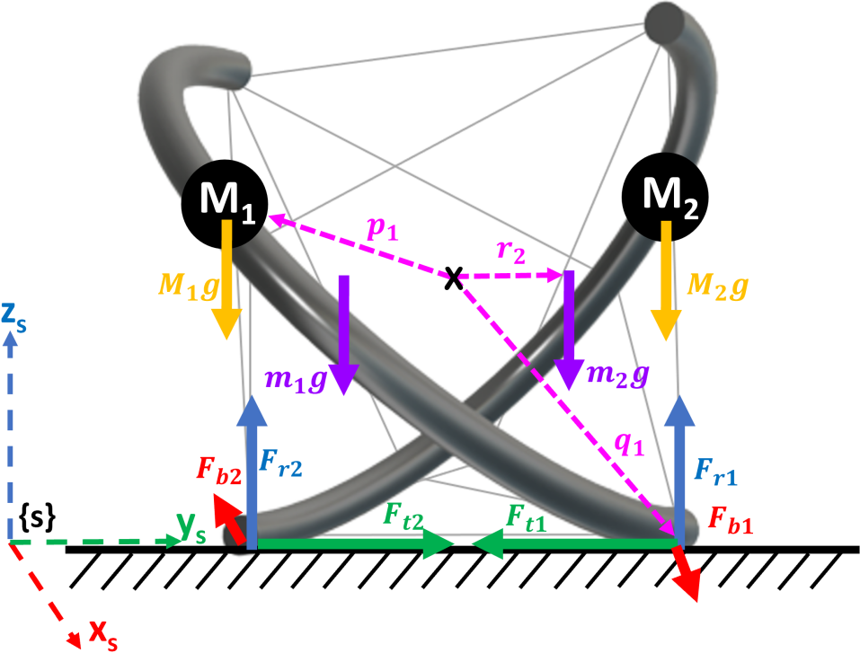
These are six equations with seven unknowns $F_{bi},F_{ti},F_{ri}$ and $\phi_{i}$ along the rolling link for the corresponding state. These can be simplified to four equations with three unknowns $F_{r1},F_{r2},\phi_{i}$ by observing that $F_{b1}=F_{b2},F_{t1}=F_{t2}$, and $Q_{1}Q_{2}$ lies in the same plane as $\bm{x}_{s},\bm{y_{s}}$, i.e., $(\hat{\bm{q}}_{1}-\hat{\bm{q}}_{2})\bm{x}_{b}=(\hat{\bm{q}}_{1}-\hat{\bm{q}}_{2})\bm{y}_{b}=0$. Hence,

$\displaystyle\begin{gathered}\begin{bmatrix}(M_{1}+M_{2}+m_{1}+m_{2})g-(F_{r1}+F_{r2})\\ \left(M_{1}g\hat{\bm{p}_{1}}+M_{2}g\hat{\bm{p}_{2}}+m_{1}g\hat{\bm{r}_{1}}+m_{2}g\hat{\bm{r}_{2}}-F_{r1}\hat{\bm{q}_{1}}-F_{r2}\hat{\bm{q}_{2}}\right)\bm{\bm{z}_{b}}\end{bmatrix}=0\end{gathered}$

Using the calculated $\bm{z}_{b}$ from Sec. II-D for each state, the ground contact angles and the reaction forces an be analytically determined as

As evident, the static analysis allows for closed form solution for $\bm{z}_{b}$. The equilibrium orientation does not provide any information about the planar position of the robot on the surface, i.e., $x,y$ components of $O_{b}$ are ‘free’ while the $z$ component is fixed at $r/\sqrt{2}$ as calculated in (14),(17). Hence, ignoring additional rotation about $\bm{z}_{s}$ the rotation matrix can be calculated using the Rodrigues’ formula and vectors $\bm{z_{s}},\bm{z_{b}}$

$\displaystyle\begin{gathered}R_{sb}(\bm{u},\theta)=I+\sin{\theta}\hat{\bm{u}}+(1-\cos{\theta})\hat{\bm{u}}^{2}\\ \mathrm{where~{}}\bm{u}=\frac{\bm{\bm{z}_{b}}\times\bm{z}_{s}}{|\bm{\bm{z}_{b}}\times\bm{z}_{s}|},\quad\theta=\mathrm{atan2}\left(|\bm{\bm{z}_{b}}\times\bm{z}_{s}|,\bm{\bm{z}_{b}}^{T}\bm{z}_{s}\right)\end{gathered}$

(47)

Rodrigues’ formula is used to convert the axis $\bm{u}$ and rotation angle $\theta$ into a rotation matrix in $SO(3)$. Additionally, $\bm{o}_{sb}^{s}=x,y,\sqrt{r}/2]^{T}$ for some $x,y$, i.e., the robot can sit anywhere on the plane. A closed form solution for $T_{sb}$ can be obtained by using the calculated $R_{sb}$ and $\bm{o}_{sb}$.

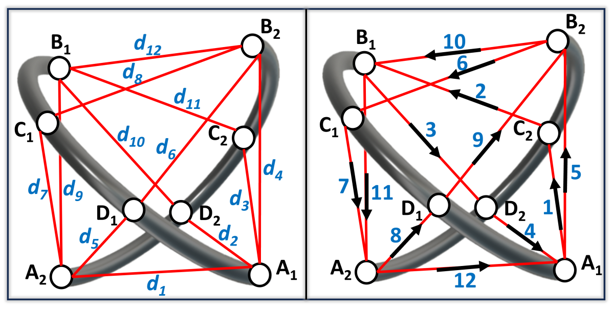
The robot is a tensegrity mechanism that combines elements of tension and compression. The shape of the robot, $T_{12}$, depends upon the cable segment lengths. Form-finding determines the lengths that dictate a desired shape. These can be found by minimizing the energy of the system [21, 22]. We define the problem in terms of the generalized coordinates, i.e., the screw $\xi$ using a Lie groups approach. The four connection points on each curved link are identical and expressed in the corresponding link coordinate systems. Consequently, the 12 cable segments are expressed as $\bm{d}\in\mathbb{R}^{12\times 4}$ and the $i$th cable $\bm{d}_{i}$ is denoted by the $i$th row

$\displaystyle\begin{gathered}\bm{d}(\xi)=PC_{1}-e^{\widehat{\xi}}PC_{2}=PC_{1}-T_{12}PC_{2}\\ P=\begin{bmatrix}\bm{p}_{A}&\bm{p}_{B}&\bm{p}_{C}&\bm{p}_{D}\\ 1&1&1&1\end{bmatrix}=\begin{bmatrix}-r&0&0&1\\ \frac{-r}{2}&\frac{-\sqrt{3}r}{2}&0&1\\ \frac{r}{2}&\frac{\sqrt{3}r}{2}&0&1\\ r&0&0&1\end{bmatrix}^{T}\end{gathered}$

(50)

where $P$ are the concatenated homogeneous representation of points $A,B,C,D$ on each arc, and the Fig. 6. The connectivity matrices $C_{1},C_{2}$ mathematically represent the two end-points each cable

$\displaystyle C_{i}[j,k]=\left\{\begin{array}[]{c@{,~}c}1\hfil,~{}&\mathrm{if~{}cable~{}k~{}contains~{}vertex~{}j~{}\mathrm{on~{}link}~{}i}\\ 0\hfil,~{}&\mathrm{otherwise}\end{array}\right.$

Now, the energy minimization problem can be written as

$\displaystyle\xi^{*}=\min_{\xi}\sum_{i=1}^{12}\frac{1}{2}k_{i}\left(|\bm{d}_{i}|-d_{0,i}\right)^{2}$

(51)

where $k_{i},d_{0,i}$ are the stiffness and the free length of the corresponding cable. There are two different free length cable segments in the system corresponding to edge-to-edge and edge-to-middle segments, $d_{0,1}=3.25"$ and $d_{0,2}=3"$. The optimal $T_{12}=e^{\widehat{\xi}}$ corresponding to the free-length matches (5) where $d_{1}=5.8551,d_{2}=5.5412$, visualized in Fig. 6(a).

Routing the cable through the two arcs such that the mechanism maintains structural integrity is challenging given the antagonistic nature of tensile cables and compressive rigid curved links. This is achieved by finding the Euler path of the graph where the connected edges and vertices correspond to the cables and connection points respectively. The reader may refer to [23] for more details. One such Euler path, $A1\rightarrow C2\rightarrow B1\rightarrow D2\rightarrow A1\rightarrow B2\rightarrow C1\rightarrow A2\rightarrow D1\rightarrow B2\rightarrow B1\rightarrow A2\rightarrow A1$, is shown in Fig. 6(b). Here, the sequence simplifies the fabrication process by ensuring the cable traverses each edge only once. Once routed, the segments are tightened until the two curved links are held in tension with the optimal cable lengths identified through form-finding.

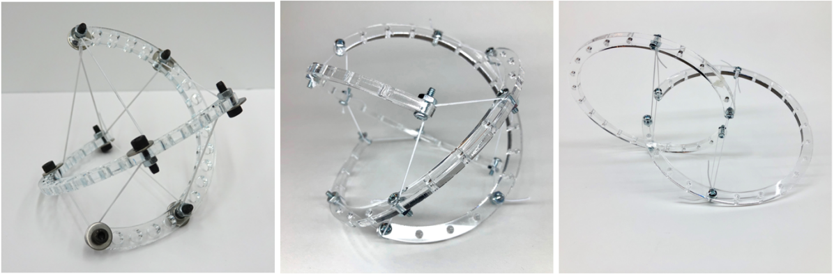
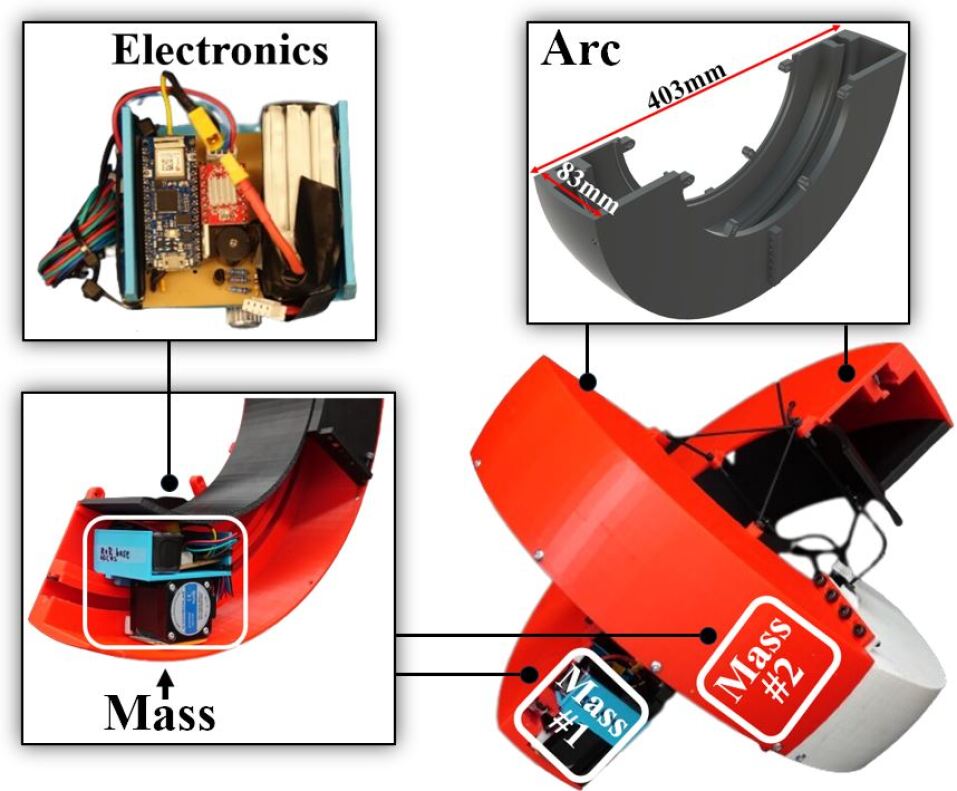
TeXploR is comprised of two 3D printed tough PLA curved links with 83mm thickness and 403mm diameter that are structurally held together with a cable using the discussed form-finding and routing approach. Motion is performed with a motor assembly traversing a GT2 timing belt running along the inside curvature of the arc. A side view of an open arc with the traveling motor assembly is shown in Fig. 7. The motor and electronic components are all positioned to one side of the timing belt with supporting delrin sliders on the top and side to maintain track alignment during movement. An Arduino Nano33 IoT, A4988 motor driver, 1,100mAh LiPo battery, and PCB are arranged compactly atop the traveling NEMA17 stepper motor. The assembly is designed with matching arc topology to reduce surface friction. Each semicircular arc weighs 431g and while each shifting mass weighs 427g, resulting in a nearly 1:1 weight ratio. The high ratio allows incremental movements of the masses to have a larger impact on the overall shifting center of mass.

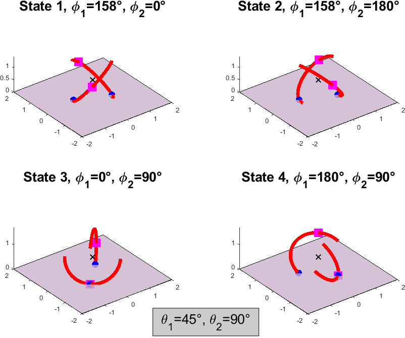
Simulations are performed in MATLAB® to obtain the equilibrium position of the robot. Given the positions of the internal masses $(\theta_{1},\theta_{2})$, the equilibrium position can be interpreted as the two points of contacts represented through ground contact angles $(\phi_{1},\phi_{2})$. These four states of the robot are analytically found using (31)-(44). As an example, Fig. 8 illustrates the four state solutions for internal mass positions $(\theta_{1},\theta_{2})=(45\degree,90\degree)$. Here, the black cross, pink squares and blue circles indicates the origin $O_{b}$ of the body coordinate system, internal masses and points of contact with the ground respectively.

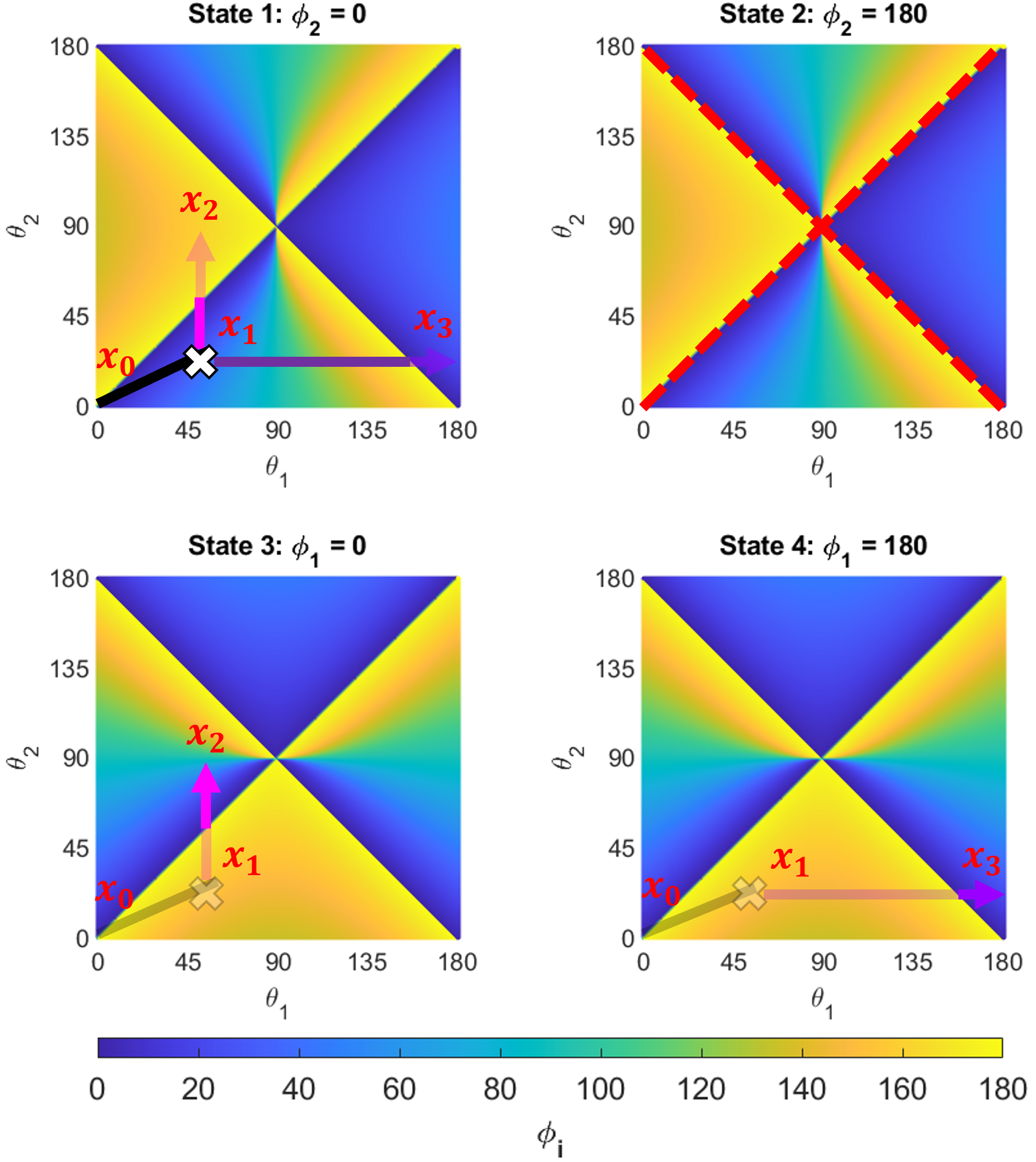
The simulated ground contact angles for the four states as a function of the internal mass positions are shown in Fig. 9. As evident from the analytical solutions, the ground contact angles for States (1, 2) and (3, 4) solutions are identical. The plots demarcate the solutions in four distinct quadrants separated by the state transition boundaries highlighted by the dotted red lines in State 2 of Fig. 9. When considering this state, the bottom and top quadrants result in more movement of the robot, i.e., greater change in $\phi_{2}$ for change in $(\theta_{1},\theta_{2})$ as compared to the left and right quadrants. The state transition boundaries represent the internal mass positions where the robot can switch states. Consider two movement sequences visualized in Fig. 9 to highlight this phenomenon. The robot starts at internal mass position $x_{0}=(0,0)$ of State 1. Next, the internal masses are quasi-statically moved to position $x_{1}$ where $\phi_{2}$ is fixed at $0\degree$. Thereafter, the robot travels along a vertical path ($\theta_{1}$ constant, $\theta_{2}$ increasing) and approaches the state transition boundary where $\phi_{1}\rightarrow 0\degree$. Instantaneously the robot enters the left quadrant of State 3 and $\phi_{1}$ begins to increase, and rolls to position $x_{2}$. The second movement again starts with the robot at position $x_{0}$ in State 1 rolling to $x_{1}$, and then begins to move towards the right state transition boundary as $\phi_{1}\rightarrow 180\degree$. The robot transitions along the boundary and instantly enters the right quadrant of State 4, stopping at $x_{3}$.

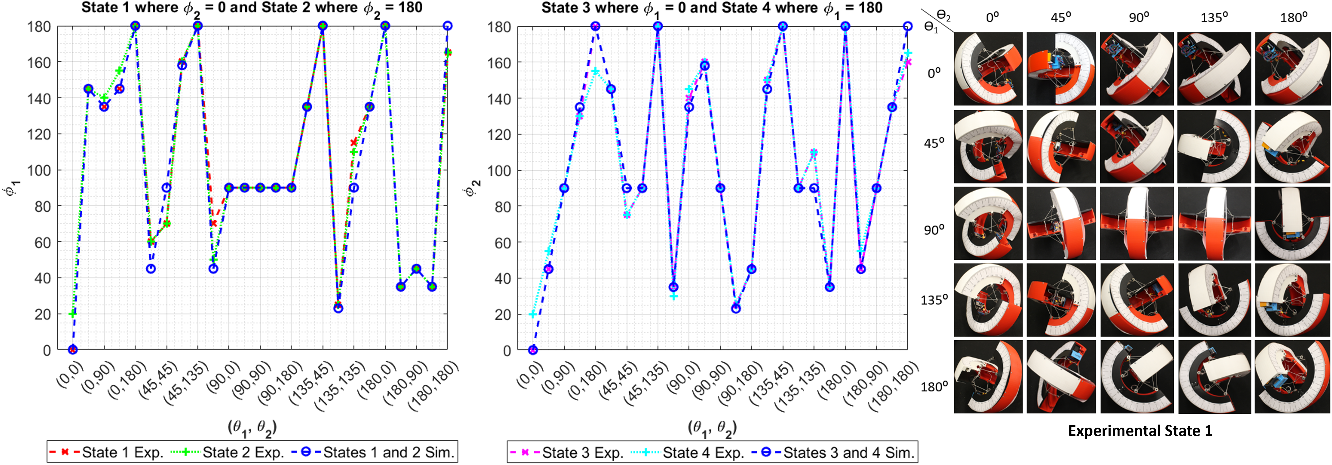
The prototype described in Sec. IV is used for experimental validation of the simulations. For combination of $(\theta_{1},\theta_{2})$ in increments of $45\degree$, the ground contact angles $(\phi_{1},\phi_{2})$ corresponding to the robot orientation were observed. Protractor strips were attached along the curved links for observing the angles. All results were compared with simulation for each state in Fig. 10(a). For most of the inputs, the $\phi_{i}$ angles match exactly. The mean absolute error (MAE) over all the inputs is $4.36\degree$. The factors contributing to these differences between real-to-sim can be attributed to the assumptions and simplifications in the model of the system. More specifically, the curved links are modeled as 2D bars with a single ground contact point, however, the prototype has an arc thickness of $83mm$ with a curved arc endpoint allowing for a range of different ground contact points. Additionally, the center of mass of each shifting mass is modeled as a point mass while the mechatronics of the shifting mass are not centered due to uneven component layout. For example, the LiPo battery is attached to one side and weighs approximately a sixth of the total shifting mass. The experimental results for each input for State 1 are shown in Fig. 10(b).

References

- [1] K. G. Gim and J. Kim, “Ringbot: Monocycle Robot With Legs,” IEEE Transactions on Robotics, vol. 40, pp. 1890–1905, 2024, conference Name: IEEE Transactions on Robotics. [Online]. Available: https://ieeexplore.ieee.org/document/10423226
- [2] U. Saranli, M. Buehler, and D. E. Koditschek, “Rhex: A simple and highly mobile hexapod robot,” The International Journal of Robotics Research, vol. 20, no. 7, pp. 616–631, 2001.
- [3] R. D. Quinn, G. M. Nelson, R. J. Bachmann, D. A. Kingsley, J. T. Offi, T. J. Allen, and R. E. Ritzmann, “Parallel complementary strategies for implementing biological principles into mobile robots,” The International Journal of Robotics Research, vol. 22, no. 3-4, pp. 169–186, 2003.
- [4] R. Chase and A. Pandya, “A Review of Active Mechanical Driving Principles of Spherical Robots,” Robotics, vol. 1, no. 1, pp. 3–23, Dec. 2012, number: 1 Publisher: Multidisciplinary Digital Publishing Institute. [Online]. Available: https://www.mdpi.com/2218-6581/1/1/3
- [5] A. Morinaga, M. Svinin, and M. Yamamoto, “A Motion Planning Strategy for a Spherical Rolling Robot Driven by Two Internal Rotors,” IEEE Transactions on Robotics, vol. 30, no. 4, pp. 993–1002, Aug. 2014.
- [6] T. Ohsawa, “Geometric Kinematic Control of a Spherical Rolling Robot,” Journal of Nonlinear Science, vol. 30, no. 1, pp. 67–91, Feb. 2020. [Online]. Available: http://link.springer.com/10.1007/s00332-019-09568-x
- [7] K. Snelson, “Snelson on the tensegrity invention,” International Journal of Space Structures, vol. 11, no. 1-2, pp. 43–48, 1996.
- [8] R. E. Skelton and M. C. De Oliveira, Tensegrity systems. Springer, 2009, vol. 1.
- [9] C. Paul, F. Valero-Cuevas, and H. Lipson, “Design and control of tensegrity robots for locomotion,” IEEE Transactions on Robotics, vol. 22, no. 5, pp. 944–957, Oct. 2006.
- [10] A. P. Sabelhaus, J. Bruce, K. Caluwaerts, P. Manovi, R. F. Firoozi, S. Dobi, A. M. Agogino, and V. SunSpiral, “System design and locomotion of SUPERball, an untethered tensegrity robot,” in 2015 IEEE International Conference on Robotics and Automation (ICRA). Seattle, WA, USA: IEEE, May 2015, pp. 2867–2873. [Online]. Available: http://ieeexplore.ieee.org/document/7139590/
- [11] K. Caluwaerts, J. Despraz, A. Işçen, A. P. Sabelhaus, J. Bruce, B. Schrauwen, and V. SunSpiral, “Design and control of compliant tensegrity robots through simulation and hardware validation,” Journal of The Royal Society Interface, vol. 11, no. 98, p. 20140520, Sep. 2014. [Online]. Available: https://royalsocietypublishing.org/doi/10.1098/rsif.2014.0520
- [12] L.-H. Chen, K. Kim, E. Tang, K. Li, R. House, E. L. Zhu, K. Fountain, A. M. Agogino, A. Agogino, V. Sunspiral, and E. Jung, “Soft Spherical Tensegrity Robot Design Using Rod-Centered Actuation and Control,” Journal of Mechanisms and Robotics, vol. 9, no. 025001, Mar. 2017. [Online]. Available: https://doi.org/10.1115/1.4036014
- [13] J. Rieffel and J.-B. Mouret, “Adaptive and resilient soft tensegrity robots,” Soft robotics, vol. 5, no. 3, pp. 318–329, 2018.
- [14] T. Rhodes, C. Gotberg, and V. Vikas, “Compact Shape Morphing Tensegrity Robots Capable of Locomotion,” Frontiers in Robotics and AI, vol. 6, 2019. [Online]. Available: https://www.frontiersin.org/articles/10.3389/frobt.2019.00111
- [15] V. Böhm, T. Kaufhold, F. Schale, and K. Zimmermann, “Spherical mobile robot based on a tensegrity structure with curved compressed members,” in 2016 IEEE International Conference on Advanced Intelligent Mechatronics (AIM), Jul. 2016, pp. 1509–1514.
- [16] V. Böhm, T. Kaufhold, I. Zeidis, and K. Zimmermann, “Dynamic analysis of a spherical mobile robot based on a tensegrity structure with two curved compressed members,” Archive of Applied Mechanics, vol. 87, no. 5, pp. 853–864, May 2017. [Online]. Available: https://doi.org/10.1007/s00419-016-1183-z
- [17] T. Kaufhold, F. Schale, V. Böhm, and K. Zimmermann, “Indoor locomotion experiments of a spherical mobile robot based on a tensegrity structure with curved compressed members,” in 2017 IEEE International Conference on Advanced Intelligent Mechatronics (AIM), Jul. 2017, pp. 523–528, iSSN: 2159-6255.
- [18] P. Schorr, E. R. C. Li, T. Kaufhold, J. A. R. Hernández, L. Zentner, K. Zimmermann, and V. Böhm, “Kinematic analysis of a rolling tensegrity structure with spatially curved members,” Meccanica, vol. 56, no. 4, pp. 953–961, Apr. 2021. [Online]. Available: https://doi.org/10.1007/s11012-020-01199-x
- [19] M. Antali and G. Stepan, “Slipping–rolling transitions of a body with two contact points,” Nonlinear Dynamics, vol. 107, no. 2, pp. 1511–1528, Jan. 2022. [Online]. Available: https://doi.org/10.1007/s11071-021-06538-5
- [20] R. M. Murray, Z. Li, and S. S. Sastry, A Mathematical Introduction to Robotic Manipulation, 1st ed. CRC Press, Dec. 2017. [Online]. Available: https://www.taylorfrancis.com/books/9781351469791
- [21] A. Tibert and S. Pellegrino, “Review of Form-Finding Methods for Tensegrity Structures,” International Journal of Space Structures, vol. 18, no. 4, pp. 209–223, Dec. 2003, publisher: SAGE Publications Ltd STM. [Online]. Available: https://doi.org/10.1260/026635103322987940
- [22] R. Connelly and W. Whiteley, “Second-Order Rigidity and Prestress Stability for TensegrityFrameworks,” SIAM Journal on Discrete Mathematics, vol. 9, no. 3, pp. 453–491, Aug. 1996. [Online]. Available: https://doi.org/10.1137/S0895480192229236
- [23] C. Woods and V. Vikas, “Design and Modeling Framework for DexTeR: Dexterous Continuum Tensegrity Manipulator,” Journal of Mechanisms and Robotics, vol. 15, no. 031006, Mar. 2023. [Online]. Available: https://doi.org/10.1115/1.4056959