Geometric phase assisted detection of Lorentz-invariance violation from modified dispersion at high energies

The Lorentz-violating quantum field theories we consider have a specific form of dispersion relation, which reads

Here $\omega_{|\mathbf{k}|}$ is the corresponding energy with the spatial momentum $\mathbf{k}$. The positive constant $M_{\star}$ determines the energy scale of Lorentz violation, and $f$ is a smooth positive function on the positive real line. Define a dimensionless quantity, $g=|\mathbf{k}|/M_{\star}$, the function $f(g)$ has the limit, $\lim_{g\rightarrow 0_{+}}f(g)\rightarrow 1$, and correspondingly the dispersion relation approaches to the Lorentz-invariant case for $g=|\mathbf{k}|/M_{\star}\ll 1$, i.e., $\omega_{|\mathbf{k}|}\approx|\mathbf{k}|$.

We assume that a real scalar field $\Phi$ can be decomposed into spatial Fourier modes such that a mode with spatial momentum $\mathbf{k}\neq 0$ is a harmonic oscillator with the angular frequency $\omega_{|\mathbf{k}|}$ shown in (1). In this case, its quantization reads

where $\textbf{x}=(x,y,z)$, $\rho_{|\textbf{k}|}=d(|\textbf{k}|/M_{\star})/\sqrt{(2\pi)^{3}|\textbf{k}|}$ is the density-of-states weight factor, which is a smooth complex-valued function on the positive real line. Note that if $f(g)=1$ and $|d(g)|=1/\sqrt{2}$, the field $\Phi$ describes the usual massless scalar field.

The detector we consider is assumed to be a two-level atom, and correspondingly its excited and ground states are respectively given by $|e\rangle$ and $|g\rangle$ with the energy-level spacing $\omega_{0}$. In order to capture the properties of Lorentz-violation in quantum field theory, we assume that the detector is coupled to the quantum field $\Phi$ shown in (2). The Hamiltonian of the whole system then reads

Here $H_{0}$ is the detector’s Hamiltonian, written as

with $\sigma_{z}$ being the Pauli matrix in $z$-component. $H_{\Phi}$ is field’s Hamiltonian, and $H_{I}$ denotes the interaction Hamiltonian between the detector and field. Specifically,

where $\mu$ is the coupling constant that usually is assumed to be small, and $\sigma_{x}=\sigma_{+}+\sigma_{-}$ is the Pauli matrix in $x$-component, with $\sigma_{+}$$(\sigma_{-})$ being the atomic rasing (lowering) operator.

At the beginning, the initial state of the detector and field is assumed to be $\rho_{\text{tot}}(0)=\rho(0)\otimes|0\rangle\langle 0|$, where $\rho(0)=|\Psi(0)\rangle\langle\Psi(0)|$, with $|\Psi(0)\rangle=\cos\frac{\theta}{2}|g\rangle+\sin\frac{\theta}{2}|e\rangle$, denotes the detector’s initial state, and $|0\rangle$ is the vacuum of the field. The dynamics of the the whole system satisfies the Liouville equation, which in the interaction picture reads

Here $\tau$ denotes the proper time of the detector. It is needed to note that in the interaction picture $H_{I}$ in (5) actually has been rotated to

shown in (6). Since we are interested in the dynamics of the detector, usually the degree of freedom of the field has to be traced over. Besides, in the limit of weak coupling, the Born approximation and Markov approximation Breuer can be used to derive the master equation of the detector. After these processes, the reduced density matrix, $\rho(\tau)$, that describes the evolving state of the detector, finally satisfies the dynamics in the Kossakowski-Lindblad form Gorini ; Lindblad ; Breuer ,

Here the effective Hamiltonian $H_{\text{eff}}=H_{0}+H_{\text{shift}}$ with the Lamb shift Breuer ; Lamb , $H_{\text{shift}}=\frac{1}{2}\mu^{2}\mathrm{Im}(\Gamma_{+}+\Gamma_{-})\sigma_{z}$, where $\Gamma_{\pm}$ will be defined below. However, usually the Lamb shift is much smaller than the energy-level spacing of the atom, $\omega_{0}$, which thus can be ignored. Furthermore, the operators in (II.2) have been defined as

with

Note that $\Delta\tau=\tau-\tau^{\prime}$ has been defined, and $G^{+}(\tau-\tau^{\prime})=\langle 0|\Phi(t(\tau),\textbf{x}(\tau))\Phi(t^{\prime}(\tau^{\prime}),\textbf{x}^{\prime}(\tau^{\prime}))|0\rangle$ is field Wightman function along the worldline of the detector $(t(\tau),\textbf{x}(\tau))$. Actually, $\gamma_{\pm}$ are the Fourier transform of the field Wightman function, denoting the detector’s transition rates.

For convenience, we can write the density matrix $\rho(\tau)$ in terms of the Pauli matrices,

where $\mathbf{I}$ is a $2\times 2$ identity matrix, and $\sigma_{i}=(\sigma_{x},\sigma_{y},\sigma_{z})$. Substituting (11) into Eq. (II.2) and using the initial state assumed before, we can finally obtain the time-dependent parameters of the reduced density matrix,

Note that here the field properties are contained in $\gamma_{\pm}$, and thus could be encoded into the state of the detector, which thus can be read out finally.

When taken around a closed trajectory in the parameter space, in addition to the dynamical phase, the state of a quantum system could acquire an additional phase factor. Since this phase depends only on the geometry of the parameter space, which is called as the GP Berry . The GP for a mixed state undergoing a non-unitary evolution is Tong

where $T$ is the evolution time of the detector, $\lambda_{k}$ and $|\phi_{k}(\tau)\rangle$ are respectively the eigenvalues and corresponding eigenvectors of the reduced density matrix $\rho(\tau)$ shown above. $|\dot{\phi}_{k}(\tau)\rangle$ is the derivative with respect to the detector’s proper time $\tau$. In order to calculate the GP of the evolving state in Eq. (11), one has to first obtain its eigenvalues, which is found to be

with $\eta=\sqrt{e^{-(\gamma_{+}+\gamma_{-})\tau}\text{sin}^{2}\theta+\omega_{3}^{2}(\tau)}$. Note that $\omega_{3}(0)=-\text{cos}\theta$, thus $\eta(0)=1$, $\lambda_{-}(0)=0$, which means it has no contribution to the GP. Therefore, we just need to consider the eigenvector corresponding to $\lambda_{+}(\tau)$, which reads

with $\theta_{\tau}$ being

According to the definition shown in Eq. (13), the GP for a time interval $T$ of evolution is

where $\Delta=(\gamma_{+}-\gamma_{-})/(\gamma_{+}+\gamma_{-})$, and $R=\text{cos}\theta+\Delta[1-e^{(\gamma_{+}+\gamma_{-})\tau}]$. Note that the GP in (17) is general. Different spacetime background and the detector’s trajectories may cuase different evolution of the detector, and thus induce different GP. Which, in turn, from the correction of the GP one can characterize the properties of spacetime background and the detector’s state of relativistic motion. In the following, we will calculate the GP for a detector which is coupled to a Lorentz-violating field and moves with a constant velocity in the $(1+3)$-dimensional Minkowski spacetime.

How the Lorentz violation affects the GP of a two-level atom (detector)? To address this issue, we will consider the detector’s dynamics introduced in section II.2, while the detector in this scenario interacts with the Lorentz-violating field described in section II.1. Furthermore, we also assume that the detector moves with a constant velocity, the corresponding trajectory reads

where $\beta$ is the rapidity with respect to the distinguished inertial frame.

Substituting the above trajectory into (II.2), we can obtain

where $\text{H}(x)$ is Heaviside function, and $g=|\textbf{k}|/M_{\star}$. For convenience, we rewrite $\gamma_{\pm}=\mu^{2}M_{\star}F_{\pm}$ with

Here $h$ is defined as a dimensionless argument: for the excitation rate $\gamma_{+}$, $h=\omega_{0}/M_{\star}$; for the deexcitation rate $\gamma_{-}$, $h=-\omega_{0}/M_{\star}$. Note that the scale parameter $M_{\star}$ enters (19) only as the overall factor and via the combination $\omega_{0}/M_{\star}$.

For the usual massless scalar field, i.e., $f(g)=1$, and $|d(g)|=1/\sqrt{2}$ in (2), we can find that $\gamma_{+}$ vanishes, which means that the detector does not become spontaneously excited. However, in this case, $\gamma_{-}=\mu^{2}\omega_{0}/2\pi$. It denotes the spontaneous decay rate of the detector and is independent of the velocity $\beta$. For the Lorentz-violating case, we can find that the crucial issue in (19) is the behavior of the argument of the Heaviside function $\mathrm{H}$: Under what condition is the argument of $\mathrm{H}$ positive for at least some interval of $g$? If $f(g)\geq 1$ for all $g$, we can find that for the $\gamma_{+}$ case, the argument of $\mathrm{H}$ always negative for all $h$. Thus the transition rate $\gamma_{+}$ vanishes, suggesting that the detector does not become spontaneously excited. However, the decay rate $\gamma_{-}$ in this case always exists and depends on the velocity of the detector as a result of the Lorentz violation.

An interesting case appears when $f(g)$ can dip somewhere below unity Husain ; Tian1 , with $f_{c}=\inf\,f$, and $0<f_{c}<1$. In this scenario, we can find that there is a critical velocity $\beta_{c}=\operatorname{arctanh}(f_{c})$, below which, i.e., $0<\beta<\beta_{c}$, $\gamma_{+}$ vanishes and thus the inertial detector moving with a constant velocity remains unexcited. The deexcitation rate is found to be $\gamma_{-}=\frac{\mu^{2}\omega_{0}}{2\pi}\{1+\cosh\beta[(1+2\cosh(2\beta))f^{\prime}(0)-2\text{Re}(d^{\prime}(0)/d(0))]h+\mathcal{O}(h^{2})\}$ for the small $\omega_{0}$ and the velocity does not approach crucial one very much, which shows that it is rapidity dependent, and the Lorentz violation is suppressed at low energies by the factor $\omega_{0}/M_{\star}$. Obviously, when $M_{\star}\rightarrow\infty$ with fixed $\omega_{0}$, it reduces to the deexcitation rate of a detector coupled to the usual massless scalar field Birrell . However, if the velocity of the detector exceeds the critical velocity, i.e., $\beta>\beta_{c}$, the argument of $\mathrm{H}$ in (20) always keeps position for $0<h<\sup_{g\geq 0}g[\sinh\beta-f(g)\cosh\beta]$, and thus $\gamma_{+}$ does not vanish. It means in this case the inertial detector with arbitrarily small positive $h$ will be excited. This is quite different from the result of the uniformly moving detector that interacts with the usual massless scalar field, which never gets spontaneously excited as discussed above. Besides, we also note that the deexcitation rate $\gamma_{-}$ in this case does not vanish and depends on the detector’s rapidities.

From the above discussions, we can find that in the presence of the Lorentz violation the transition rate of the inertially moving detector may depend on the detector’s rapidity, which is different from the Lorentz invariant case, where the detector’s transition rate is rapidity-independent. Particularly, if a quantum field with the dispersion in (1) satisfies the conditions: the smooth positive-valued function $f(g)\rightarrow 1$ as $g\rightarrow 0_{+}$, and $f_{c}=\inf\,f$ yielding $0<f_{c}<1$, and $|d(g)|\rightarrow 1/\sqrt{2}$ as $x\rightarrow 0_{+}$, $d(g)$ is nonvanishing everywhere, an inertial UDW detector with rapidity $\beta>\beta_{c}=\operatorname{arctanh}(f_{c})$ in the preferred frame experiences spontaneous excitation at arbitrarily low $\omega_{0}$. However, this never occurs in the Lorentz-invariant quantum field theory. Furthermore, both the excitation and deexcitation rates are proportional to the Lorentz violation energy scale $M_{\star}$. Since the GP is sensitive to transition rates and from the above analysis the transition rates becomes significantly modified by the Lorentz violation and the detector’s velocity, we expect the Lorentz-violating component of the GP to be correspondingly modified. Besides, the accumulative nature of the GP Eduardo1 ; Arya could facilitate the detection of weak effects such as the Lorentz-violating modifications to the field.

For convenience, we rewrite the deexcitation rate of the detector coupled to the usual massless scalar quantum field as $\gamma_{0}=\frac{\mu^{2}\omega_{0}}{2\pi}$. Then the transition rates for the Lorentz-violating case in Eqs. (19) and (20) can be rewritten as

where $c_{\pm}=\pm\frac{2\pi F_{\pm}}{h}$ are dimensionless functions which are determined by the detector’s rapidity $\beta$ and the detector’s energy-level spacing $|h|$. Since the parameter $\gamma_{0}/\omega_{0}=\mu^{2}/2\pi$ is small, we can Taylor expand the GP in (17) to the first order of $\gamma_{0}/\omega_{0}$ Hu ; James ; Tian3 ; Arya . For the uniformly moving detector coupled to a quantum field with Lorentz-invariant dispersion, we can obtain the corresponding GP,

where $\varphi=\omega_{0}T$. The first term $\Omega_{D}=-\varphi\text{cos}^{2}\frac{\theta}{2}$ in (22) denotes the GP of an isolated detector, and second term is the correction, $\delta\Omega_{I}=\varphi^{2}\frac{\gamma_{0}}{8\omega_{0}}\text{sin}^{2}\theta(\text{cos}\theta-2)$, as a result of the interaction between detector and quantum field. Here the GP for Lorentz-invariant field theory case just depends on the accumulation time, the initial state and energy-level spacing of the detector, and the coupling strength between the detector and field.

If an uniformly moving detector is coupled to a quantum field with a dispersion in (1), we can obtain the corresponding GP of the detector, which is Taylor expanded to the first order of $\gamma_{0}/\omega_{0}$,

The first term denotes the GP of an isolated detector, $\Omega_{D}=-\varphi\text{cos}^{2}\frac{\theta}{2}$. The second term is the correction to the GP that arises from the interaction between detector and external quantum field, which is given by

This correction is quite different from that of the Lorenz-invariant case. Besides the accumulation time, the initial state and energy-level spacing of the detector, and the coupling strength between the detector and field, it also depends on the rapidity of the detector, seen from (19). Note that the rapidity-dependent property of the GP results from the Lorentz violation.

From the above analysis, it is found that when a quantum field is of a Lorentz-violating dispersion, the detector that the field is coupled to could acquire a correction of GP which depends on the detector’s rapidity. However, for the Lorentz invariant case, the corresponding GP correction is independent of the rapidity. Therefore, whether the GP is rapidity dependent could be used as a criteria to characterize the Lorentz violation. Due to this feature, the GP here can be used to probe the Lorentz violation with the assistance of the detector’s rapidity. Besides, the GP could be accumulative, this nature may also facilitate the detection of weak effects. In what follows, we will apply the above analysis to a concrete example—to the detection of the polymer quantization motivated by loop quantum gravity.

The Wightman function in polymer quantum field theory reads Mortuza

Here, $\Delta E_{n}(|\mathbf{k}|)=E_{n}(|\mathbf{k}|)-E_{0}(|\mathbf{k}|)$, with

and $\psi_{n}$ are given by

satisfying the Mathieu equation, referring to Ref. Mortuza for the details. $B_{n}(x)$ and $A_{n}(x)$ are the Mathieu characteristic value functions, $\mathrm{ce}_{n}(x,q)$ and $\mathrm{se}_{n}(x,q)$ are respectively the elliptic cosine and sine functions.

Substituting the detector’s trajectory in (18) into the above Wightman function in (25), we can straightly calculate the transition rates in (II.2) of the inertially moving detector that is coupled to a scalar field in polymer quantum field theory,

where $\omega_{n}(g)=\Delta E_{n}(g)/M_{\star}$. Since only nonzero matrix elements are $c_{4n+3}$ (for $n=0,1,2,\cdots$) Mortuza , the above transition rates (31) can be rewritten as

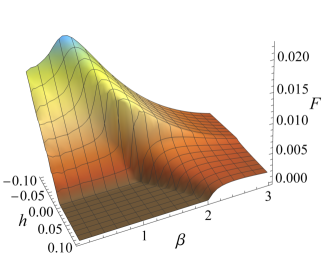
If the polymer quantization is real, the deexcitation rate of the detector may depend on the polymer energy scale $M_{\star}$ (may be identified as Planck energy) and the detector’s rapidity, $\beta$. Which never happens for the usual massless quantum scaler field theory. Furthermore, it has been demonstrated in Refs. Husain ; Nirmalya1 ; Jorma ; Nirmalya2 that in the polymer quantum field theory even an inertially moving detector with a constant velocity can still get excited when its rapidity exceeds a critical one. This comes from the fact that the dispersion in the polymer quantum field theory, $\Delta E_{3}$ in (32), may satisfy the excitation condition of an inertial detector discussed in Section II.4. Numerical calculations show that in this case the critical velocity is found to be $\beta_{c}\approx 1.3675$. To better understand the excitation and deexcitation rates of the inertial detector in the polymer quantum field theory, in Fig. 1 we plot them as a function of the detector’s energy-level spacing $|h|$ and detector’s rapidity $\beta$. It is found that there is a critical velocity only beyond which the detector could get excited. However, the deexcitation rate always exists and depends on the detector’s velocity.

Since the detector’s transition rates presence quite different behavior when below and beyond the critical velocity $\beta_{c}$ for arbitrary small $h$, in what follows we will separately investigate the GP acquired by the detector for two cases: 1) $\beta<\beta_{c}$; 2) $\beta>\beta_{c}$.

As discussed above, when the detector’s velocity is below the critical one $\beta_{c}$, the detector then does not get excited, and correspondingly $c_{+}$ in (21) vanishes. Therefore, in this case only $c_{-}$ related to the deexcitation rate has the contribution to the GP acquired by the detector. Note that the accumulation time, seen from Eq. (24), can only change the magnitude of the GP correction from the interaction between detector and field, while does not change its behavior. Therefore, here we choose the evolution time $T=2\pi/\omega_{0}$ just for an example, to explore how the detector’s energy-level spacing $|h|$ and its velocity $\beta$ affect the GP.

Fixing a typical coupling constant $\mu\sim 10^{-3}$, in Fig. 2 the GP correction (shown in Eq. (24)) of the detector as a function of the detector’s energy-level spacing $|h|$ and its velocity $\beta$ (below the critical one $\beta_{c}$) is plotted with different initial state cases, $\theta=(\pi/6,\pi/3,\pi/2)$ (see (II.2) when $\tau=0$). It is found that for different initial states the GP corrections share similar behavior, while have different magnitudes. One can also find this result from Eq. (24), actually $\delta\Omega_{V}=\varphi^{2}\frac{\gamma_{0}}{8\omega_{0}}\sin^{2}\theta(\cos\theta-2)c_{-}$ in this case. Furthermore, near the critical velocity, it is shown that the GP is quite sensitive to the polymer quantization for smaller $h$. This is because that as shown in Eq. (21) $c_{-}=-2\pi F_{-}/h$ is proportional to $1/h$, and the transition rate $F_{-}$ behaves sharply as a function of the velocity $\beta$ in the small $h$ and critical velocity nearby region shown in Fig. 1. Since $|h|=\omega_{0}/M_{\star}$, the above result alternatively means that for fixed $\omega_{0}$ the GP may be sensitive to larger possible $M_{\star}$. Actually, in the polymer quantum field theory, the polymer energy scale $M_{\star}$ may be identified as the Planck energy, that is thought to be huge in theory. In this sense, the GP seems to be quite sensitive to the polymer quantization theory.

If the detector’s velocity exceeds the critical value $\beta_{c}$, as discussed above the inertial detector could get excited for arbitrary small energy-level spacing $\omega_{0}$ case, and correspondingly the excitation rate $c_{+}$ exists. Therefore, in this case both the excitation rate and the deexcitation rate have the contribution to the GP shown in (24). As a result of that, one can expect that compared with the $\beta<\beta_{c}$ case, the GP for the $\beta>\beta_{c}$ case may present different behavior as a function of the detector’s energy-level spacing $|h|$ and its velocity $\beta$.

In Fig. 3, we also take the evolution time $T=2\pi/\omega_{0}$ and the coupling strength $\mu\sim 10^{-3}$, and plot the GP correction (shown in Eq. (24)) of the detector as a function of the detector’s energy-level spacing $|h|$ and its velocity $\beta$ (above the critical one $\beta_{c}$) for different initial state cases, $\theta=(\pi/6,\pi/3,\pi/2)$ (see (II.2) when $\tau=0$). We can find that the GP exhibits quite different behavior compared to the $\beta<\beta_{c}$ case shown in Fig. 2. The maximum GP correction is acquired in arbitrary small $h$ region, while the corresponding optimal velocity (determinate the maximum GP correction) is the critical one or others, which depends on the initial state of the detector. Note that this is because the excitation and deexcitation rates have unsymmetry responses to the detector’s energy-level spacing $|h|$ and its velocity $\beta$ shown in Fig. 1. Furthermore, for high velocity and large energy-level spacing, the GP correction approaches to vanishment. It means it is quite difficult to detect the polymer quantization theory using the GP method in this case. Therefore, when the velocity exceeds the critical one, to find the maximum GP one needs to consider the initial state of the detector, and properly design the detector with the energy-level spacing $|h|$.

In order to comparatively study how the GP is influenced in the whole velocity regime (both below and above the critical one), in Fig. 4 we plot this GP as a function of the detector’s velocity $\beta$ for initial state $\theta\approx 0.569\pi$ with different fixed energy-level spacing $|h|$. The evolution time $T=2\pi/\omega_{0}$, the coupling strength $\mu\sim 10^{-3}$ have been taken. Here we can find that if velocity is much below the critical one the GP is insensitive to the velocity, and is much smaller than that in other velocity regime. In this case, we can obtain an approximate GP as, $\delta\Omega_{V}=\varphi^{2}\frac{\gamma_{0}}{8\omega_{0}}\sin^{2}\theta(\cos\theta-2)[1+2\cosh\beta\sinh^{2}\beta h+\mathcal{O}(h^{2})]$ for small $|h|$. Near the critical velocity, $\beta_{c}\approx 1.3675$, the GP shows a drastic behavior—increasing sharply as a function of the velocity. This means the GP is quite sensitive to the polymer quantization near the critical velocity. This has been discussed in Section III.2. However, when the velocity exceeds the critical one, $c_{+}=\frac{2\pi F_{+}}{h}$ presents a drastic behavior as a function of the velocity $\beta$, and in this case both $c_{+}$ and $c_{-}$ have the contribution to the GP. Therefore, the GP behaves sharply near the critical velocity. Besides, it is found that when the velocity is above the critical one, the amount of the GP is much larger than that for the quite small velocity case (below the critical velocity). Which is more distinct for smaller $|h|$ case. This is because that when above the critical velocity, although $|h|$ is small, both $F_{\pm}$ have finite values shown in Fig. 1 and $c_{\pm}=\pm\frac{2\pi F_{\pm}}{h}$ are proportional to $1/|h|$. This means when above the critical velocity the GP may be susceptible for smaller $|h|$ case. Alternatively, with fixed $\omega_{0}$ the GP might be quite sensitive to the polymer quantization due to $|h|=\omega_{0}/M_{\star}$.

Above analysis raises an interesting question: can the inertial detector moving with a constant velocity far below the critical one acquire a measurable GP? Seen from Eq. (24), the GP correction is proportional to $\varphi^{2}=(\omega_{0}T)^{2}$, thus the GP could be accumulative. In this regard, one can expect that this accumulation nature may assist the inertial detector moving with a constant velocity far below the critical one to acquire a measurable GP. In Fig. 5, we choose a fixed energy-level spacing $|h|$, the fixed velocity $\beta$ below the critical one and the optimal initial state $\theta\approx 0.569\pi$, and plot the GP correction shown in (24) as a function of the effective accumulation time $\varphi$. We can find that with the increase of the accumulation time, the GP correction increases monotonously.

As an example, we will choose some experimentally feasible quantities and numerically estimate the possible bound of the polymer scale $M_{\star}$ that could be constrained using the GP method when the velocity much below the critical one (e.g., the velocity $\beta\in[0,10^{-3}]$). Specifically, if we take the currently feasible quantities $\omega_{0}\sim 10^{9}\text{Hz}$, $\mu\sim 10^{-3}$, initial state $\theta\approx 0.569\pi$, and the accumulative time $T=10^{7}\times 2\pi/\omega_{0}$ in the experiment, we can find that for the possible $M_{\star}\in[10^{13},10^{25}]\text{GeV}$ regime by bound (which means that $|h|$ ranges from $10^{-40}$ to $10^{-28}$), the GP acquired is found to be $[10^{-32},10^{-20}]$, which is much smaller than the minimum magnitude of GP that could be measurable with current technology. Therefore, when the velocity is much smaller than the critical one, it seems to be impossible to detect the polymer quantization using the GP method. However, if the much longer coherent time of quantum system can be maintained for the future experiments, e.g., longer than $T=10^{7}\times 2\pi/\omega_{0}$ by several orders, possible polymer quantization scale discussed above might be experimentally testable using the GP method, as shown in Fig. 5.

Fortunately, as discussed above the GP near the critical velocity is quite sensitive to the polymer quantization. We wonder whether it is possible to acquire a measurable GP in this case. For $\beta=1.3674642$ below the crucial velocity (the more precise value of the critical one is $\beta_{c}=1.367464205629544$), we also take $\omega_{0}\sim 10^{9}\text{Hz}$, $\mu\sim 10^{-3}$, initial state $\theta\approx 0.569\pi$ and the accumulative time $T=10^{7}\times 2\pi/\omega_{0}$, we can find that if the experimentally detectable GP is $10^{-8}$, then the possible testable lower bound of $|h|$ is $6.97\times 10^{-10}$, equivalently the polymer quantization scale $M_{\star}\sim 10^{-6}\text{GeV}$. This quantity seems quite small compared with the possible values discussed above. However, we need to note that the chosen velocity $\beta=1.3674642$ actually is not close enough to the critical value such that the transition rate occurs outside the drastic response regime of velocity. This is because that the smaller $|h|$ is, the more drastically the transition rate changes with respect to the velocity below the critical one. Moreover, the drastic change point of the transition rate becomes closer to the critical velocity when $|h|$ is smaller. One can see this from Fig. 1. To obtain a tighter bound on the polymer quantization scale $M_{\star}$ using the GP method, the chosen velocity should be as close as possible to the critical one, while whose precision is beyond our calculation. When the detector’s velocity exceeds the critical one, $\beta_{c}$, in theory arbitrary $M_{\star}$ could be testable by appropriately choosing the energy-level spacing $\omega_{0}$, the accumulative time $T$, and the initial state of the detector. Note that although this critical velocity seems to be quite large, actually it is smaller than the possible velocity to which the ions could be accelerated at the Relativistic Heavy Ion Collider Husain .