Geometric Characterization of the $H$ -property for Step-graphons

Mohamed-Ali Belabbas¹¹1M.-A. Belabbas is with the Department of Electrical and Computer Engineering and the Coordinated Science Laboratory, University of Illinois, Urbana-Champaign. Email: [email protected]. and Xudong Chen²²2X. Chen is with the Department of Electrical, Computer, and Energy Engineering, University of Colorado Boulder. Email: [email protected].

Abstract

²²footnotetext: M.-A. Belabbas and X. Chen contributed equally to the manuscript in all categories.

In a recent paper [1], we have exhibited a set of conditions that are necessary for the $H$ -property to hold for the class of step-graphons. In this paper, we prove that these conditions are essentially sufficient.

1 Introduction and Main Result

In [1], we introduced the so-called $H$ -property for a graphon $W$ — roughly speaking, it is the property that a graph $G$ sampled from $W$ admits a Hamiltonian decomposition a.s.. The presence of a Hamiltonian decomposition in a graph underlies a number of important properties pertinent to structural system theory, such as structural controllability [2] and structural stability [3, 4]. See [1] for details. In that same paper, we have exhibited a set of conditions that were necessary for the $H$ -property to hold for the class of step-graphons. We show in this paper that these conditions are also essentially (in a sense made precise below) sufficient.

$H$ -property: We start by recalling the definitions of a graphon and its sampling procedure. A graphon is a symmetric, measurable function $W:[0,1]^{2}\to[0,1]$ . Step-graphons, along with their partitions, are defined below:

Definition 1 (Step-graphon and its partition).

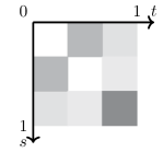
A graphon $W$ is a step-graphon if there exists an increasing sequence $0=\sigma_{0}<\sigma_{1}<\cdots<\sigma_{q}=1$ such that $W$ is constant over each rectangle $[\sigma_{i},\sigma_{i+1})\times[\sigma_{j},\sigma_{j+1})$ for all $0\leq i,j\leq q-1$ . We call $\sigma=(\sigma_{0},\sigma_{1},\ldots,\sigma_{q})$ a partition for $W$ .

Graphons can be used to sample undirected graphs. Other uses of graphons in system theory as limits of adjacency matrices can be found in [5, 6, 7]. In this paper, we denote by $G_{n}\sim W$ graphs $G_{n}$ on $n$ nodes sampled from a graphon $W$ . The sampling procedure was introduced in [8, 9] and is reproduced below: Let $\mathrm{Uni}[0,1]$ be the uniform distribution on $[0,1]$ . Given a graphon $W$ , a graph $G_{n}=(V,E)\sim W$ on $n$ nodes is obtained as follows:

1.

Sample $y_{1},\ldots,y_{n}\sim\mathrm{Uni}[0,1]$ independently. We call $y_{i}$ the coordinate of node $v_{i}\in V$ .
2.

For any two distinct nodes $v_{i}$ and $v_{j}$ , place an edge $(v_{i},v_{j})\in E$ with probability $W(y_{i},y_{j})$ .

It should be clear that if $0\leq p\leq 1$ is a constant and $W(s,t)=p$ for all $(s,t)\in[0,1]^{2}$ , then $G_{n}\sim W$ is an Erdős-Rényi random graph with parameter $p$ . Consequently, graphons can be seen as a way to introduce inhomogeneity in the edge densities between different pairs of nodes.

Let $W$ be a graphon and $G_{n}\sim W$ . In the sequel, we use the notation $\vec{G}_{n}=(V,\vec{E})$ to denote the directed version of $G_{n}$ , defined by the edge set

\vec{E}:=\{v_{i}v_{j},v_{j}v_{i}\mid(v_{i},v_{j})\in E\}.

(1)

In words, we replace an undirected edge $(v_{i},v_{j})$ with two directed edges $v_{i}v_{j}$ and $v_{j}v_{i}$ . The directed graph $\vec{G}_{n}$ is said to have a Hamiltonian decomposition if it contains a subgraph $H$ , with the same node set of $\vec{G}$ , such that $H$ is a node disjoint union of directed cycles. See Fig. 1 for illustration.

(a)

(b)

Figure 1: Left: An undirected graph

G

4

nodes. Right: The directed graph

\vec{G}

obtained from

G

by replacing every undirected with two oppositely oriented edges. The cycle

D_{1}=v_{1}v_{2}v_{3}v_{4}v_{1}

forms a Hamiltonian decomposition of

\vec{G}

. The two node disjoint cycles

D_{2}=v_{1}v_{2}v_{1}

and

D_{3}=v_{3}v_{4}v_{2}

also form a Hamiltonian decomposition of

\vec{G}

We now have the following definition:

Definition 2 ( $H$ -property).

Let $W$ be a graphon and $G_{n}\sim W$ . Then, $W$ has the $H$ -property if

\lim_{n\to\infty}\mathbb{P}(\vec{G}_{n}\mbox{ has a Hamiltonian decomposition})=1.

(2)

We will see below that the $H$ -property is essentially a “zero-one” property in a sense that the probability on the left hand side of (2) converges to either $0$ or $1$ .

Key objects: We present three key objects associated with a step-graphon, namely, its concentration vector, its skeleton graph, and its associated edge polytope, all of which were introduced in [1].

Definition 3 (Concentration vector).

Let $W$ be a step-graphon with partition $\sigma=(\sigma_{0},\ldots,\sigma_{q})$ . The associated concentration vector $x^{*}=(x^{*}_{1},\ldots,x^{*}_{q})$ has entries defined as follows: $x^{*}_{i}:=\sigma_{i}-\sigma_{i-1}$ , for all $i=1,\ldots,q$ .

It should be clear from the sampling procedure above that the concentration vector describes the proportion of sampled nodes in each interval $[\sigma_{i},\sigma_{i+1})$ .

Given a step-graphon, its support can be described by a graph, which we call skeleton graph:

Definition 4 (Skeleton graph).

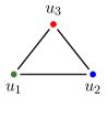
To a step-graphon $W$ with a partition $\sigma=(\sigma_{0},\ldots,\sigma_{q})$ , we assign the undirected graph $S=(U,F)$ on $q$ nodes, with $U=\{u_{1},\ldots,u_{q}\}$ and edge set $F$ defined as follows: there is an edge between $u_{i}$ and $u_{j}$ if and only if $W$ is non-zero over $[\sigma_{i-1},\sigma_{i})\times[\sigma_{j-1},\sigma_{j})$ . We call $S$ the skeleton graph of $W$ for $\sigma$ .

We illustrate the relationship between a step-graphon and its skeleton graph in Figure 2.

Without loss of generality and for ease of presentation, we will consider throughout this paper step-graphons $W$ whose skeleton graphs are connected. Though there is no unique skeleton graph associated to a step-graphon (since there are infinitely many different partitions for $W$ ), we show in Proposition 1 that if one such skeleton graph is connected, then so are all the others. For $S$ not connected, it is not too hard to see that the corresponding step-graphon is block-diagonal. Our results apply naturally to every connected component of $S$ .

We decompose the edge set of $S$ as $F=F_{0}\cup F_{1}$ , where elements of $F_{0}$ are self-loops, and elements of $F_{1}$ are edges between distinct nodes. We also introduce the subset $F_{2}\subseteq F_{1}$ of edges that are not incident to two nodes with self-loops.

Let $\mathcal{I}:=\{1,\ldots,|F|\}$ be an index set for $F$ (so that the edges are now ordered). We decompose $\mathcal{I}$ similarly: let $\mathcal{I}_{0}$ , $\mathcal{I}_{1}$ , and $\mathcal{I}_{2}$ index $F_{0}$ , $F_{1}$ , and $F_{2}$ respectively.

To introduce the edge-polytope of $S$ , we recall that the incidence matrix $Z=[z_{ij}]$ of $S$ is an $|U|\times|F|$ matrix with its entries defined as follows:

z_{ij}:=\frac{1}{2}\begin{cases}2,&\text{if }f_{j}\in F_{0}\text{ is a loop on node }u_{i},\\ 1,&\text{if node }u_{i}\text{ is incident to }f_{j}\in F_{1},\\ 0,&\text{otherwise}.\end{cases}

(3)

Owing to the factor $\frac{1}{2}$ in (3), all columns of $Z$ are probability vectors, i.e., all entries are nonnegative and sum to one. The edge polytope of $S$ was introduced in [10] and the definition is reproduced below (with a slight difference in inclusion of the factor $\frac{1}{2}$ of the generators $z_{j}$ ):

Definition 5 (Edge polytope).

Let $S=(U,F)$ be a skeleton graph and $Z$ be the associated incidence matrix. Let $z_{j}$ , for $1\leq j\leq|F|$ , be the columns of $Z$ . The edge polytope of $S$ , denoted by $\mathcal{X}(S)$ , is the convex hull of the vectors $z_{j}$ :

\mathcal{X}(S):=\operatorname{conv}\{z_{j}\mid j=1,\ldots,|F|\}.

(4)

A point $x\in\mathcal{X}(S)$ is said to be in the relative interior of $\mathcal{X}(S)$ , denoted by $\operatorname{int}\mathcal{X}(S)$ , if there exists an open neighborhood $U$ of $x$ in $\mathbb{R}^{q}$ (with $q=|U|$ ) such that $U\cap\mathcal{X}(S)\subseteq\mathcal{X}(S)$ . If $x$ is not an interior point, then it is called a boundary point and we write $x\in\partial\mathcal{X}(S)$ .

Main result: Let $W$ be a step-graphon. For a given partition $\sigma$ for $W$ , let $x^{*}$ and $S$ be the associated concentration vector and the skeleton graph (which is assumed to be connected). We say that a cycle in $S$ is odd if it contains an odd number of distinct nodes (or edges); with this definition, self-loops are odd cycles. Given these, we state the following two conditions:

Condition A: The graph $S$ has an odd cycle.

Condition B: The vector $x^{*}$ belongs to $\operatorname{int}\mathcal{X}(S)$ .

The two conditions are stated in terms of a partition $\sigma$ and its induced skeleton graph and edge-polytope. As mentioned earlier, there exist infinitely many partitions for a given step-graphon. However, the following proposition states that the two above conditions are invariant under changes of a partition.

Proposition 1.

Let $W$ be a step-graphon. For any two partitions $\sigma$ and $\sigma^{\prime}$ for $W$ , let $x^{*}$ , $x^{\prime*}$ be the corresponding concentration vectors and let $S$ , $S^{\prime}$ be the corresponding skeleton graphs. Then, the following hold:

1.

$S$ is connected if and only if $S^{\prime}$ is;
2.

$S$ has an odd cycle if and only if $S^{\prime}$ does;
3.

$x^{*}\in\mathcal{X}(S)$ (resp. $x^{*}\in\operatorname{int}\mathcal{X}(S)$ ) if and only if $x^{\prime*}\in\mathcal{X}(S^{\prime})$ (resp. $x^{\prime*}\in\mathcal{X}(S^{\prime})$ ).

We refer the reader to Appendix A for a proof of the proposition.

We are now in a position to state the main result:

Main Theorem.

Let $W$ be a step-graphon. If it satisfies Conditions A and B for a given (and, hence, any) partition $\sigma$ , then it has the $H$ -property.

Remark 1.

In our earlier work [1], we have shown that if a step-graphon $W$ has the $H$ -property, then it is necessary that Condition A and the following hold:

Condition B’: The vector $x^{*}$ belongs to $\mathcal{X}(S)$ .

Note that condition B’ is weaker than Condition B: Specifically, Condition B leaves out the set of step-graphons for which $x^{*}\in\partial\mathcal{X}(S)$ , which is a set of measure zero. For step-graphons satisfying Conditions A and B’, but not B, it is possible that

\lim_{n\to\infty}\mathbb{P}(\vec{G}_{n}\sim W\mbox{ has a Hamiltonian decomposition})\in(0,1).

We have produced explicit examples of such step-graphon in [11, 1].

Outline of proof: Given a step-graphon $W$ with skeleton graph $S$ , and $G_{n}\sim W$ , the sampling procedure induces a natural graph homomorphism $\pi:G_{n}\to S$ , whereby all nodes $v_{j}$ of $G_{n}$ whose coordinates $y_{j}$ belong to $[\sigma_{i-1},\sigma_{i})$ are mapped to $u_{i}$ . With a slight abuse of notation, we will use the same letter $\pi$ to denote the homomorphism $\pi:\vec{G}_{n}\to\vec{S}$ .

Let $n_{i}(G_{n}):=|\pi^{-1}(u_{i})|$ be the number of nodes whose coordinates belong to $[\sigma_{i-1},\sigma_{i})$ . We call the following vector the empirical concentration vector of $G_{n}$ :

x(G_{n}):=\frac{1}{n}(n_{1}(G_{n}),\ldots,n_{q}(G_{n})).

(5)

The proof of the Main Theorem contains three steps, outlined below, among which step 2 contains the bulk of the proof.

Step 1: The proof starts by showing how conditions $A$ and $B$ imply that the empirical concentration vector eventually belongs to the edge polytope. First, it should be clear that the edge polytope $\mathcal{X}(S)$ is a subset of the standard simplex $\Delta^{q-1}$ in $\mathbb{R}^{q}$ ; thus, $\dim\mathcal{X}(S)\leq(q-1)$ . Condition A, owing to [10], is both necessary and sufficient for the equality to hold. Next, note that $nx(G_{n})=(n_{1}(G_{n}),\ldots,n_{q}(G_{n}))$ is a multinomial random variable with $n$ trials and $q$ outcomes with probabilities $x^{*}_{i}$ , for $1\leq i\leq q$ . Then, Condition B guarantees, via Chebyshev’s inequality, that $x(G_{n})$ belongs to $\operatorname{int}\mathcal{X}(S)$ a.s. — in this paper, a.s. stands for almost surely as $n\to\infty$ .

The next two steps are then dedicated to establishing the following fact:

x(G_{n})\in\operatorname{int}\mathcal{X}(S)\\ \Rightarrow G_{n}\mbox{ admits a Hamiltonian decomposition {\em a.s.}.}

(6)

Step 2: We start by working under the assumption that $W$ is a binary step-graphon, i.e., $W(s,t)\in\{0,1\}$ for almost all $(s,t)\in[0,1]^{2}$ . In this case, we will see that a sampled graph $G_{n}\sim W$ is completely determined by its empirical concentration vector $x(G_{n})$ . Consequently, our task (establishing (6)) is reduced to establishing the following:

x(G_{n})\in\operatorname{int}\mathcal{X}(S)\mbox{ and $n$ is sufficiently large}\\ \Rightarrow G_{n}\mbox{ admits a Hamiltonian decomposition surely.}

(7)

The proof of (7) is constructive. An important object that will arise therefrom is what we call the $A$ -matrix assigned to every Hamiltonian decomposition $H$ for $\vec{G}_{n}$ , written as a map $\rho(H)=A$ .

Specifically, the matrix $A$ is a $q$ -by- $q$ matrix whose $ij$ th entry tallies the number of edges of $H$ that go from a node in $\pi^{-1}(u_{i})$ to a node in $\pi^{-1}(u_{j})$ (A precise definition is in Subsection 2.1 and see Figure 3 for an illustration). Any such matrix is then shown to satisfy a number of enviable properties, among which we have $\rho(H){\bf 1}=x(G_{n})$ .

In a nutshell, we have just created the following sequence of maps:

H\xmapsto{}\rho(H)\xmapsto{}\rho(H){\bf 1}=x(G_{n}),

with the domain being all Hamiltonian decompositions in $\vec{G}_{n}$ , for any $G_{n}$ sampled from a given binary graphon.

Now, the effort in establishing (7) is to create appropriate right-inverses (at least locally) of the maps in the above sequence, i.e., we aim to create maps $x\mapsto A(x)$ and $\tilde{\rho}:A(x)\mapsto H$ with the property that $\rho\cdot\tilde{\rho}$ is the identity map and $A(x){\bf 1}=x$ . The map $x\mapsto A(x)$ is created in Proposition 2, Subsection 2.3, and the map $\tilde{\rho}$ is created in Proposition 3, Subsection 2.4. From these two subsections, it will be clear that by introducing the $A$ -matrix as an intermediate object, we can decouple the analytic part of the proof, contained in the creation of the map $x\mapsto A(x)$ , from the graph-theoretic part, contained in the creation of $\tilde{\rho}$ . This will conclude the proof of (7).

Step 3: To close gap between binary step-graphons and general ones, we introduce here an equivalence relation on the class of step-graphons, namely, two step-graphons $W_{1}$ and $W_{2}$ are equivalent if their supports are the same. Or, said otherwise, $W_{1}$ and $W_{2}$ are equivalent if they share the same concentration vector and skeleton graph. Note, in particular, that each equivalence class $[W]$ contains a unique representative which is a binary step-graphon, denoted by $W^{s}$ . We then establish (6) by showing that $W$ has the $H$ -property if and only if $W^{s}$ does. In essence, we show that the $H$ -property is decided completely by the concentration vector and the skeleton graph of a step-graphon $W$ .

The proof of this statement builds upon several classical results from random graph theory, and is presented in Subsection 2.5.

Notation: We gather here key notations and conventions.

Graph theory: Let $G=(V,E)$ be an undirected graph. Graphs in this paper do not have multiple edges, but may have self-loops. We denote edges by $(v_{i},v_{j})\in E$ ; if $v_{i}=v_{j}$ , then we call the edge a self-loop. For a given node $v_{i}$ , let $N(v_{i}):=\{v_{j}\in V\mid(v_{i},v_{j})\in E\}$ be the neighbor set of $v_{i}$ . The degree of $v_{i}$ , denoted by $\deg(v_{i})$ , is the cardinality of $N(v_{i})$ .

We will also deal with directed graphs (digraphs) in this paper. Whether a graph is directed or undirected will be clear from the context and/or notation. We denote by $v_{i}v_{j}$ the directed edge from $v_{i}$ to $v_{j}$ ; we call $v_{j}$ an out-neighbor of $v_{i}$ and $v_{i}$ an in-neighbor of $v_{j}$ . Similarly, we define $N_{+}(v_{i})$ and $N_{-}(v_{i})$ the sets of in-neighbors and out-neighbors of $v_{i}$ , respectively.

Recall that for a given undirected graph $G=(V,E)$ , possibly with self-loops, we let $\vec{G}=(V,\vec{E})$ be the directed graph defined as in (1). Self-loops in $\vec{G}$ are the same as the ones in $G$ , i.e., they are not duplicated.

A closed walk in a graph (or digraph) is an ordered sequence of nodes $v_{1}v_{2}\cdots v_{k}v_{1}$ in $G$ (resp. $\vec{G}$ ) so that all consecutive nodes are ends of some edges (resp. directed edges). A cycle is a closed walk without repetition of nodes in the sequence except the starting- and the ending-nodes. For clarity of the presentation, we use letter $C$ to denote cycles in undirected graphs and the letter $D$ for cycles in directed graphs.

Miscellaneous: We use $\mathbf{1}$ to denote a column vector of all $1$ , whose dimension will be clear within the context. We write $x\leq y$ for vectors $x,y\in\mathbb{R}^{q}$ if the inequality holds entrywise. For a given vector $x\in\mathbb{R}^{q}$ , we denote its $\ell_{1}$ normalization by $\bar{x}$ , i.e., $\bar{x}:=\frac{x}{\|x\|_{1}}$ , with the convention that $\bar{0}=0$ . Further, given the vector $x$ , we denote by $[x]$ the vector whose entry $[x]_{i}$ is a closest integer to $x_{i}$ for $1\leq i\leq q$ where for the case $x_{i}=k+\frac{1}{2}$ , with $k$ an integer, we set $[x]_{i}:=k$ . We denote the standard simplex in $\mathbb{R}^{q}$ by $\Delta^{q-1}:=\{x\in\mathbb{R}^{q}\mid x\geq 0\mbox{ and }x^{\top}{\bf 1}=1\}$ . Finally, given a $q\times q$ matrix $A$ , we denote by $\operatorname{supp}A$ its support, i.e., the set of indices corresponding to its non-zero entries.

2 Analysis and Proof of the Main Theorem

Throughout the proof, $W$ is a step-graphon, $\sigma$ its associated partition, and $S=(U,F)$ its skeleton graph on $q$ nodes, which has an odd cycle. Let $F_{0}$ and $F_{1}$ be given as after Definition 4. We can naturally associate to them the subgraphs

S_{0}:=(U,F_{0})\quad\mbox{and}\quad S_{1}:=(U,F_{1}).

(8)

Note that $S$ has an odd cycle if and only if $S_{0}$ is edgewise non-empty or $S_{1}$ has an odd cycle. The lemma below states that we can consider, without loss of generality, only the latter case of $S_{1}$ containing an odd cycle.

Lemma 1.

Let $W$ be a step-graphon. If $W$ admits a partition $\sigma$ with skeleton graph $S$ containing an odd cycle, then $W$ admits a partition $\sigma^{\prime}$ with skeleton graph $S^{\prime}$ so that the subgraph $S^{\prime}_{1}$ has an odd cycle.

The proof of the lemma can be established by using the notion of “one-step refinement” introduced in Appendix A for the partition $\sigma$ : If $S_{1}$ already has an odd cycle, then there is nothing to prove. Otherwise, consider a one-step refinement on a node with self-loop in $S$ , which will yield a cycle of length $3$ in $S^{\prime}$ .

2.1 On the edge polytope $\mathcal{X}(S)$

Rank of $\mathcal{X}(S)$ : Recall that $\mathcal{X}(S)$ is the edge-polytope of $S$ . Similarly, we let $\mathcal{X}(S_{i})$ , for $i=1,2$ , be the edge polytope (see Definition 5) of $S_{i}$ , i.e., $\mathcal{X}(S_{i})$ is the convex hull of the $z_{j}$ ’s, with $j\in{\cal I}_{i}$ , where ${\cal I}_{i}$ indexes edges in $F_{i}$ .

We call $x$ an extremal point of a polytope $\mathcal{X}$ if there is no line segment in $\mathcal{X}$ that contains $x$ in its interior. The maximal set of extremal points is called the set of extremal generators for $\mathcal{X}$ . The following result characterizes the extremal generators of $\mathcal{X}(S_{0})$ , $\mathcal{X}(S_{1})$ , and of $\mathcal{X}(S)$ :

Lemma 2.

The set of extremal generators of $\mathcal{X}(S_{i})$ , for $i=1,2$ , is $\{z_{j}\mid j\in\mathcal{I}_{i}\}$ . The set of extremal generators of $\mathcal{X}(S)$ is $\{z_{i}\mid i\in\mathcal{I}_{0}\cup\mathcal{I}_{2}\}$ . .

Proof.

The statement for $\mathcal{X}(S_{0})$ is obvious from the definition of the corresponding $z_{i}$ . For $\mathcal{X}(S_{1})$ , it suffices to see that the vectors $z_{i}$ , for $i\in{\cal I}_{1}$ , have exactly two non-negative entries, and the supports of these vectors are pairwise distinct. Hence, if $z_{i}=\sum_{j\in{\cal I}_{1}}c_{i}z_{j}$ with $c_{j}\geq 0$ , we necessarily have $c_{j}=0$ for $j\neq i$ and $c_{i}=1$ . For $\mathcal{X}(S)$ , we refer the reader to [1, Proposition 1] for a proof.

The rank of a polytope $\mathcal{X}$ is the dimension of its relative interior. It is known [10] that if $S$ has $q$ nodes, then

\operatorname{rank}\mathcal{X}(S)=\begin{cases}q-1&\mbox{if $S$ has an odd cycle},\\ q-2&\mbox{otherwise.}\end{cases}

(9)

Equivalently, we have the following result [12] on the rank of the incidence matrix $Z_{S}$ of $S$ :

\operatorname{rank}Z_{S}=\begin{cases}q&\mbox{if $S$ has an odd cycle},\\ q-1&\mbox{otherwise.}\end{cases}

(10)

The $A$ -matrix: Let $G_{n}\sim W$ and suppose that $\vec{G}_{n}$ has a Hamiltonian decomposition, denoted by $H$ .

Recall that $\pi:\vec{G}_{n}\to\vec{S}$ is the graph homomorphism introduced above (5). Let $n_{ij}(H)$ be the number of (directed) edges of $H$ from a node in $\pi^{-1}(u_{i})$ to a node in $\pi^{-1}(u_{j})$ . It is not hard to see that (see [1, Lemma 1] for a proof) for all $u_{i}\in U$ ,

n_{i}(G_{n})=\sum_{u_{j}\in N(u_{i})}n_{ij}(H)=\sum_{u_{j}\in N(u_{i})}n_{ji}(H).

(11)

We now assign to the skeleton graph $S$ a convex set that will be instrumental in establishing the main result:

Definition 6 ( $A$ -matrices and their set).

Let $S=(U,F)$ be an undirected graph on $q$ nodes. We define $\mathcal{A}(S)$ as the set of $q\times q$ nonnegative matrices $A=[a_{ij}]$ satisfying the following two conditions:

1.

If $(u_{i},u_{j})\notin F$ , then $a_{ij}=0$ ;
2.

$A{\bf 1}=A^{\top}{\bf 1}$ , and ${\bf 1}^{\top}A{\bf 1}=1$ .

Because every defining condition for ${\cal A}(S)$ is affine, the set $\mathcal{A}(S)$ is a convex set.

Now, to each Hamiltonian decomposition $H$ of $\vec{G}_{n}$ , we assign the following $q\times q$ matrix:

\rho(H):=\frac{1}{n}\left[n_{ij}(H)\right]_{1\leq i,j\leq q}.

(12)

It follows from (11) that $\rho(H)\in\mathcal{A}(S)$ and $\rho(H){\bf 1}=x(G_{n})$ . Furthermore, we have established in [1, Proposition 4] the following connection between the set $\mathcal{A}(S)$ and the edge polytope $\mathcal{X}(S)$ :

\mathcal{X}(S)=\{x\in\mathbb{R}^{q}\mid x=A{\bf 1}\mbox{ for some }A\in\mathcal{A}(S)\}.

(13)

We refer the reader to Figure 3 for illustration.

2.2 Local coordinate systems on $\mathcal{X}(S)$ and $\mathcal{X}(S_{1})$

This section establishes the groundwork for the construction of the map $x\mapsto A(x)$ described in the proof outline. To this end, we first show how to express any point in a neighborhood ${\cal U}$ of $x^{*}\in\mathcal{X}(S)$ as a positive combination of the columns of the incidence matrix $Z_{S}$ . This amounts to solving the linear equations $Z_{S}\phi(x)=x$ , for $x\in{\cal U}$ , with $\phi(x)$ being continuous in $x$ and positive. We will solve a similar problem for $y^{*}\in\mathcal{X}(S_{1})$ and with $Z_{S}$ replaced by $Z_{S_{1}}$ , and we call the corresponding solution $\theta(y)$ . These two maps will be put to use in the next subsection.

Construction of the map $\phi$ : We start with the following lemma:

Lemma 3.

Suppose that $S=(U,F)$ has an odd cycle. Then, for any $x^{*}\in\operatorname{int}\mathcal{X}(S)$ , there exist a closed neighborhood $\mathcal{U}$ of $x^{*}$ in the simplex and a continuous map $\phi:\mathcal{U}\to\operatorname{int}\Delta^{|F|-1}$ such that $Z_{S}\phi(x)=x$ for any $x\in\mathcal{U}$ .

Proof.

Because $\mathcal{X}(S)$ is finitely generated by the columns of $Z_{S}$ , i.e. the $z_{i}$ ’s for $i\in{\cal I}$ , and because $x^{*}\in\operatorname{int}\mathcal{X}(S)$ , there exists a positive probability vector $c:=(c_{1},\ldots,c_{|F|})$ such that $x^{*}=Z_{S}c$ . Let $\epsilon:=\frac{1}{2}\min_{i\in{\cal I}}\{c_{i}\}$ . Because $S$ has at least one odd cycle, we know from (10) that $Z_{S}$ is full rank. Thus, we can pick $q$ columns, say $z_{1},\ldots,z_{q}$ of $Z_{S}$ , that form a basis of $\mathbb{R}^{q}$ . Let $B\subset\mathbb{R}^{|F|}$ be a closed ball centered at $0$ with radius $\epsilon$ , and let

B_{0}:=\{y\in B\mid{\bf 1}^{\top}y=0\mbox{ and }y_{i}=0,\mbox{ for all }i>q\}.

The dimension of $B_{0}$ is $(q-1)$ . We now define the map

\psi:B_{0}\to\mathbb{R}^{q}:y\mapsto x^{*}+Z_{S}y=Z_{S}(y+c).

It should be clear that $\psi$ is a linear bijection between $B_{0}$ and its image $\psi(B_{0})$ . By the construction of $B$ and $B_{0}$ , all the entries of $(y+c)$ , for $y\in B_{0}$ , are positive and, moreover, ${\bf 1}^{\top}(y+c)=1$ . It then follows that the image of $\psi$ is a closed neighborhood of $x^{*}$ inside $\mathcal{X}(S)$ . We now set $\phi:=\psi^{-1}$ . It remains to show that $\phi(x)\in\Delta^{|F|-1}$ . This holds because every column of $Z_{S}$ belongs to $\Delta^{q-1}$ and so does $x$ . Thus, from $Z_{S}\phi(x)=x$ , we have that $x$ is a convex combination of the columns of $Z_{S}$ , which implies that $\phi(x)\in\Delta^{|F|-1}$ .

Let $x^{*}\in\operatorname{int}\mathcal{X}(S)$ and $\phi$ be the map given in Lemma 3. For an edge $f_{i}$ of $S$ , we let $\phi_{i}$ be the corresponding entry of $\phi$ . We next define two functions $\tau_{i}:\mathcal{U}\to\mathbb{R}^{q}$ , for $i=1,2$ , as follows:

\tau_{i}(x):x\mapsto\sum_{j\in{\cal I}_{i}}\phi_{j}(x)z_{j}.

(14)

If $S$ has no self-loops, then $\tau_{0}$ is set to be the zero map. We can thus decompose $x\in\mathcal{U}$ as

x=\tau_{0}(x)+\tau_{1}(x).

We record the following simple observation for later use:

Lemma 4.

Let ${\cal U}$ be as in Lemma 3. For every $x\in{\cal U}$ , the set of indices of nonzero (positive) entries of $\tau_{0}(x)$ is $\{i\mid u_{i}\mbox{ has a self-loop}\}$ and, moreover, every entry of $\tau_{1}(x)$ is positive.

Proof.

The statement for $\tau_{0}(x)$ is trivial. The statement for $\tau_{1}(x)$ follows from the fact that $\phi(x)$ has positive entries and no row of $Z_{S_{1}}$ is identically $0$ .

Construction of the map $\theta$ : For any $x\in{\cal U}$ , let $\bar{\tau}_{i}(x)$ , for $i=0,1$ , be defined as follows:

\bar{\tau}_{i}(x):=\begin{cases}\tau_{i}(x)/\|\tau_{i}(x)\|_{1}&\mbox{if }\tau_{i}(x)\neq 0,\\ 0&\mbox{otherwise}.\end{cases}

Since $S$ has odd cycle, recall that we can assume by Lemma 1 that $S_{1}$ has an odd cycle. Thus, by (9), the rank of $\mathcal{X}(S_{1})$ is $(q-1)$ . In particular, it implies that the relative interior of $\mathcal{X}(S_{1})$ is open in $\Delta^{q-1}$ . Further, by Lemma 4, if $x\in{\cal U}$ , then $\bar{\tau}_{1}(x)\in\operatorname{int}\mathcal{X}(S_{1})$ .

The map $\theta$ we introduce below is akin to the map $\phi$ introduced in Lemma 3, but defined on a closed neighborhood of

\bar{x}_{1}^{*}:=\bar{\tau}_{1}(x^{*})\in\operatorname{int}\mathcal{X}(S_{1}).

Lemma 5.

Suppose that $S$ (and, hence, $S_{1}$ ) has an odd cycle; then, for the given $\bar{x}^{*}_{1}\in\operatorname{int}\mathcal{X}(S_{1})$ , there exist a closed neighborhood ${\cal V}$ of $\bar{x}_{1}^{*}$ in $\Delta^{q-1}$ and a continuous map $\theta:{\cal V}\to\operatorname{int}\Delta^{|F_{1}|-1}$ such that $Z_{S_{1}}\theta(y)=y$ for any $y\in{\cal V}$ .

The proof is entirely similar to the one of Lemma 3, and is thus omitted.

Because $\phi$ and $\theta$ are both positive, continuous maps over closed, bounded domains, there exists an $\alpha\in(0,1)$ so that

	$\displaystyle\phi(x)\geq\alpha{\bf 1}\mbox{ for all }x\in{\cal U},$		(15)
	$\displaystyle\theta(x)\geq\alpha{\bf 1}\mbox{ for all }x\in{\cal V}.$		(15)

On the image of $\bar{\tau}_{1}$ : For a given $x^{*}\in\operatorname{int}\mathcal{X}(S)$ , the domains of $\phi$ and $\theta$ are closed neighborhoods ${\cal U}$ and ${\cal V}$ of $x^{*}$ and $\bar{x}_{1}^{*}$ , respectively. Later in the analysis, we will pick an arbitrary $x\in{\cal U}$ and apply $\theta$ to $\bar{\tau}_{1}(x)$ . For this, we need that $\bar{\tau}_{1}(x)$ belongs to ${\cal V}$ . To this end, we will shrink ${\cal U}$ so that $\bar{\tau}_{1}({\cal U})\subseteq{\cal V}$ and thus the composition $\theta\bar{\tau}_{1}$ is well defined. In fact, we have the stronger statement:

Lemma 6.

Let $\alpha>0$ be given as in (15). There exist a closed neighborhood ${\cal U}^{\prime}\subseteq{\cal U}$ of $x^{*}$ and a positive $\epsilon<\frac{1}{4}\alpha$ , such that

\overline{\tau_{1}(x)+\eta}=\frac{\tau_{1}(x)+\eta}{\|\tau_{1}(x)+\eta\|_{1}}\in{\cal V},

for any $x\in{\cal U}^{\prime}$ and for any $\eta\in\mathbb{R}^{q}$ with $\|\eta\|_{\infty}\leq\epsilon$ .

Proof.

Let ${\cal V}^{\prime}$ be a closed ball centered at $\bar{x}_{1}^{*}$ and contained in the interior of ${\cal V}$ . Then, it is known [13, Theorem 4.6] that there exists an $\epsilon^{\prime}>0$ such that the $\epsilon^{\prime}$ -neighborhood of ${\cal V}^{\prime}$ , with respect to the infinity norm, is contained in the interior of ${\cal V}$ . Let ${\cal U}^{\prime}:=\bar{\tau}_{1}^{-1}({\cal V}^{\prime})$ and $\epsilon$ be sufficiently small so that

\frac{(8+4\alpha)\epsilon}{q\alpha^{2}}<\min\left\{\epsilon^{\prime},\frac{1}{4}\alpha\right\}.

(16)

We claim that the above-defined ${\cal U}^{\prime}$ and $\epsilon$ are as desired.

Since $\bar{\tau}_{1}$ is continuous and since ${\cal V}^{\prime}$ is a closed ball centered at $\bar{x}^{*}_{1}$ , ${\cal U}^{\prime}$ is a closed neighborhood of $x^{*}$ . Now, pick an arbitrary $x\in{\cal U}^{\prime}$ . For ease of notation, we set $x_{1}:=\tau_{1}(x)$ and $\bar{x}_{1}=\bar{\tau}_{1}(x)$ for the remainder of this proof. Then,

$\displaystyle\left\\|\overline{x_{1}+\eta}-\bar{x}_{1}\right\\|_{\infty}$	$\displaystyle=\left\\|\frac{x_{1}+\eta}{\\|x_{1}+\eta\\|_{1}}-\frac{x_{1}}{\\|x_{1}\\|_{1}}\right\\|_{\infty}$
	$\displaystyle=\left\\|\frac{(\\|x_{1}\\|_{1}-\\|x_{1}+\eta\\|_{1})x_{1}+\\|x_{1}\\|_{1}\eta}{\\|x_{1}+\eta\\|_{1}\\|x_{1}\\|_{1}}\right\\|_{\infty}$
	$\displaystyle\leq\frac{\|\\|x_{1}\\|_{1}-\\|x_{1}+\eta\\|_{1}\|}{\\|x_{1}+\eta\\|_{1}\\|x_{1}\\|_{1}}\\|x_{1}\\|_{\infty}+\frac{\\|\eta\\|_{\infty}}{\\|x_{1}+\eta\\|_{1}}$
	$\displaystyle\leq\frac{\|\\|x_{1}\\|_{1}-\\|x_{1}+\eta\\|_{1}\|}{\\|x_{1}+\eta\\|_{1}\\|x_{1}\\|_{1}}+\frac{\\|\eta\\|_{\infty}}{\\|x_{1}+\eta\\|_{1}}$	(17)

where we used the fact that $\|x_{1}\|_{\infty}\leq 1$ to obtain the last inequality. To further evaluate (2.2), we first note that

|\|x\|_{1}-\|x_{1}+\eta\|_{1}|\leq\|\eta\|_{1}\leq q\|\eta\|_{\infty}\leq q\epsilon.

Next, by (3), (14) and (15), every entry of $x_{1}$ is greater than $\frac{1}{2}\alpha$ , so $\|x_{1}\|_{1}\geq\frac{1}{2}q\alpha$ . Moreover, since $\epsilon<\frac{1}{4}\alpha$ ,

\|x_{1}+\eta\|_{1}\geq\|x_{1}\|_{1}-\|\eta\|_{1}\geq\frac{1}{2}q\alpha-q\epsilon\geq\frac{1}{4}q\alpha.

Finally, using (16), we can proceed from (2.2) and obtain that

\left\|\overline{x_{1}+\eta}-\bar{x}_{1}\right\|_{\infty}\leq\frac{8\epsilon}{q\alpha^{2}}+\frac{4\epsilon}{q\alpha}=\frac{(8+4\alpha)\epsilon}{q\alpha^{2}}<\epsilon^{\prime},

which implies that $\overline{x_{1}+\eta}$ belongs to the $\epsilon^{\prime}$ -neighborhood of ${\cal V}^{\prime}$ and, hence, to ${\cal V}$ .

Remark 2.

From now on, to simplify the notation, we denote by ${\cal U}$ the set ${\cal U}^{\prime}$ of Lemma 6.

2.3 Construction of the map $x\mapsto A(x)$

To construct the map, we first specify its domain, which will be a subset of ${\cal U}$ . If $x\in\mathbb{R}^{q}$ is an empirical concentration vector of some $G_{n}\sim W$ for a step-graphon $W$ , then $nx$ necessarily has integer entries. Define a subset of ${\cal U}$ as follows:

{\cal U}^{*}:=\left\{x\in{\cal U}\mid nx\in\mathbb{Z}^{q}_{+}\mbox{ for some }n\in\mathbb{Z}_{+}\right\},

(18)

where $\mathbb{Z}_{+}$ is the set of positive integers.

Since the analysis for the $H$ -property will be carried out in the asymptotic regime $n\to\infty$ , the relevant empirical concentration vectors are those of $G_{n}$ for $n$ large. To this end, let $\alpha\in(0,1)$ be such that (15) is satisfied and $\epsilon$ be as in Lemma 6. We have the following definition:

Definition 7.

Given an $x\in{\cal U}^{*}$ , $n\in\mathbb{Z}_{+}$ is paired with $x$ if $n>\frac{8}{\alpha\epsilon}$ and $nx$ is integer valued.

With the above, we now state the main result of this subsection:

Proposition 2.

Let $S=(U,F)$ be a connected undirected graph, with at least one odd cycle, and $\vec{S}=(U,\vec{F})$ be its directed version. Then, there exist a map $A:{\cal U}^{*}\mapsto\mathcal{A}(S)$ and a positive number $\underline{a}$ such that for any $x\in{\cal U}^{*}$ and for any $n$ paired with $x$ , the following hold:

1.

$A(x){\bf 1}=x$ ;
2.

$nA(x)$ is integer-valued and $n\operatorname{diag}A(x)$ has even entries;
3.

$n\|\operatorname{diag}A(x)-\tau_{0}(x)\|_{\infty}\leq 1$ , where $\tau_{0}$ is defined in (14);
4.

$n|a_{ij}(x)-a_{ji}(x)|\leq 1$ for all $1\leq i,j\leq q$ ;
5.

For any $u_{i}u_{j}\in\vec{F}$ , $a_{ij}(x)>\underline{a}$ .

Note that item 5 and the fact that $A(x)\in\mathcal{A}(S)$ imply $\operatorname{supp}A(x)=\vec{S}$ , i.e., $a_{ij}\neq 0$ if and only if $u_{i}u_{j}\in\vec{F}$ .

The proof of Proposition 2 is constructive. It will rely on a few technical facts we establish here. Let $x\in{\cal U}^{*}$ and $n$ be paired with $x$ . Define

\tau^{\prime}_{0}(x):=\frac{2}{n}\left[\frac{n}{2}\tau_{0}(x)\right]\quad\mbox{and}\quad\tau^{\prime}_{1}(x):=x-\tau^{\prime}_{0}(x),

(19)

where we recall that the operation $\left[\,\cdot\,\right]$ is the integer-rounding operation, introduced in the notation of Section 1. The vector $n\tau_{0}^{\prime}(x)$ is then the vector with even entries closest to the entries of $n\tau_{0}(x)$ . Next, we define

n^{\prime}_{0}:=n\|\tau^{\prime}_{0}(x)\|_{1}\mbox{ and }n^{\prime}_{1}:=n\|\tau^{\prime}_{1}(x)\|_{1}

(20)

Recall that $\bar{\tau}^{\prime}_{0}$ and $\bar{\tau}^{\prime}_{1}$ are the $\ell_{1}$ normalization of $\tau^{\prime}_{0}$ and $\tau^{\prime}_{1}$ , respectively. It should be clear from the construction that $n^{\prime}_{0}+n_{1}^{\prime}=n$ and

\bar{\tau}^{\prime}_{i}=\frac{n}{n^{\prime}_{i}}\tau^{\prime}_{i},\mbox{ for }i=1,2.

For a given $x\in{\cal U}^{*}$ , there obviously exist infinitely many positive integers $n$ that are paired with $x$ . However, the ratios $n^{\prime}_{0}/n$ and $n^{\prime}_{1}/n$ are independent of $n$ and determined completely by $x$ .

We also need the following lemma:

Lemma 7.

The following items hold:

1.

For $i=1,2$ , $\operatorname{supp}\tau^{\prime}_{i}(x)=\operatorname{supp}\tau_{i}(x)$ and, moreover, the nonzero entries of $\tau^{\prime}_{i}(x)$ are uniformly bounded below by $\frac{1}{2}(1-\epsilon/4)\alpha$ .
2.

The ratio $n^{\prime}_{0}/n$ is bounded below by $(1-\epsilon/8)\alpha|F_{0}|$ . The ratio $n_{1}^{\prime}/n$ is bounded below by $3q\alpha/8$ .
3.

Let ${\cal V}$ be defined as in Lemma 5. Then, $\bar{\tau}_{1}(x)\in{\cal V}$ .

We provide a proof of the lemma in Appendix B.

With the lemma above, we now establish Proposition 2:

Proof of Proposition 2.

We start by defining two matrix-valued functions $A_{0}(x)$ and $A_{1}(x)$ so that for any $x\in{\cal U}^{*}$ , $A_{i}(x)\in\mathcal{A}(S)$ and ${A_{i}}(x){\bf 1}=\bar{\tau}^{\prime}_{i}(x)$ . We will then let $A(x)$ be the convex combination of these two matrices given by

A(x)=\frac{n^{\prime}_{0}}{n}A_{0}(x)+\frac{n_{1}^{\prime}}{n}A_{1}(x).

(21)

Since $\mathcal{A}(S)$ is convex, it will then follow that $A(x)\in\mathcal{A}(S)$ .

Construction of $A_{0}$ : The matrix $A_{0}(x)$ is simply given by

A_{0}(x):=\operatorname{diag}\bar{\tau}^{\prime}_{0}(x).

(22)

By Lemma 4, $\operatorname{supp}\tau_{0}(x)$ is constant over ${\cal U}$ . By the first item of Lemma 7, $\operatorname{supp}\tau_{0}(x)=\operatorname{supp}\tau^{\prime}_{0}(x)$ for all $x\in{\cal U}^{*}$ . It then follows that $\operatorname{supp}A_{0}(x)$ is also constant over ${\cal U}^{*}$ . By the same item, the nonzero entries of $A_{0}(x)$ are uniformly bounded below by a positive constant.

Construction of $A_{1}$ : The construction is more involved than the one of $A_{0}$ , and requires to first define the intermediate matrix $A^{\prime}_{1}$ . To this end, recall that $Z_{S_{1}}$ is the edge-incidence matrix of $S_{1}=(U,F_{1})$ , obtained by removing the self-loops of $S$ , and that $\theta$ is the map given in Lemma 5, i.e., $Z_{S_{1}}\theta(y)=y$ for all $y\in{\cal V}$ . Given an edge $f=(u_{i},u_{j})\in S_{1}$ , we denote by $\theta_{f}(y)$ the corresponding entry of $\theta(y)$ . By item 3 of Lemma 7, $\bar{\tau}^{\prime}_{1}(x)$ belongs to ${\cal V}$ , which is the domain of $\theta$ . Now, we define the symmetric matrix $A^{\prime}_{1}(x)=[a^{\prime}_{1,ij}(x)]\in\mathbb{R}^{q\times q}$ as follows:

a^{\prime}_{1,ij}(x):=\begin{cases}\frac{1}{2}\theta_{f}(\bar{\tau}^{\prime}_{1}(x))&\mbox{if }f=(u_{i},u_{j})\in F_{1},\\ 0&\mbox{otherwise}.\end{cases}

(23)

In particular, the diagonal of $A^{\prime}_{1}$ is $0$ , and so will be the diagonal of $A_{1}$ as shown below. From the definition of the incidence matrix $Z_{S_{1}}$ and (23), we have that $A^{\prime}_{1}(x){\bf 1}=Z_{S_{1}}\theta(\bar{\tau}^{\prime}_{1}(x))$ . By Lemma 5, $Z_{S_{1}}\theta(\bar{\tau}^{\prime}_{1}(x))=\bar{\tau}^{\prime}_{1}(x)$ . It then follows that

A^{\prime}_{1}(x){\bf 1}=\bar{\tau}^{\prime}_{1}(x),

(24)

and, hence, ${\bf 1}^{\top}A^{\prime}_{1}(x){\bf 1}={\bf 1}^{\top}\bar{\tau}^{\prime}_{1}(x)=1$ . Furthermore, since $A^{\prime}_{1}(x)$ is symmetric, ${A^{\prime}_{1}(x)}{\bf 1}=A^{\prime}_{1}(x)^{\top}{\bf 1}$ . We thus have that $A^{\prime}_{1}(x)\in\mathcal{A}(S)$ . Since $\theta_{f}$ is positive for every $f\in F_{1}$ , $\operatorname{supp}A^{\prime}_{1}(x)$ is constant over ${\cal U}$ . Moreover, by (15), the nonzero entries of $A^{\prime}_{1}(x)$ are uniformly bounded below by $\frac{1}{2}\alpha$ .

Next, we use $A^{\prime}_{1}$ to construct $A_{1}$ . There are two cases; one is straightforward and the other is more involved:

Case 1: $n_{1}^{\prime}A^{\prime}_{1}(x)$ is integer-valued: Set $A_{1}(x):=A^{\prime}_{1}(x)$ .

Case 2: $n_{1}^{\prime}A^{\prime}_{1}(x)$ is not integer-valued: In this case, we appeal to the result [14, Theorem 2]: There, we have shown that there exists a matrix $A_{1}(x)=[a_{1,ij}(x)]$ in $\mathcal{A}(S)$ , with

A_{1}(x){\bf 1}=A^{\prime}_{1}(x){\bf 1}=\bar{\tau}^{\prime}_{1}(x)

(25)

such that $A_{1}(x)$ has the same support as $A^{\prime}_{1}(x)$ and

n_{1}^{\prime}a_{1,ij}(x)=\lfloor n_{1}^{\prime}a^{\prime}_{1,ij}(x)\rfloor\quad\mbox{or}\quad n_{1}^{\prime}a_{1,ij}(x)=\lceil n_{1}^{\prime}a^{\prime}_{1,ij}(x)\rceil.

In particular, $n_{1}^{\prime}A_{1}(x)$ is integer-valued. Because $a^{\prime}_{1,ij}(x)=a^{\prime}_{1,ji}(x)$ , it follows that

n_{1}^{\prime}|a_{1,ij}(x)-a_{1,ji}(x)|\leq 1,\quad\forall 1\leq i,j\leq q.

(26)

Moreover, if $a^{\prime}_{1,ij}(x)>0$ , then

a_{1,ij}(x)>a^{\prime}_{1,ij}(x)-\frac{1}{n_{1}^{\prime}}\geq\alpha-\frac{1}{n_{1}^{\prime}}\geq\alpha-\frac{1}{n}\frac{n}{n_{1}^{\prime}}\geq\alpha-\frac{8}{3nq\alpha}>\left(1-\frac{1}{12q}\right)\alpha.

(27)

where second to the last inequality follow from item 2 of Lemma 7 and the last inequality follows from the hypothesis on $n$ (specifically $n>\frac{8}{\alpha\epsilon}$ ) from the statement and the condition that $\epsilon<\alpha/4$ from Lemma 6.

Proof that $A$ satisfies the five items of the statement:

1.

From (22), $A_{0}(x){\bf 1}=\bar{\tau}^{\prime}_{0}(x)$ . For $A_{1}$ , it was shown that $A_{1}(x){\bf 1}=\bar{\tau}^{\prime}_{1}(x)$ in (24) and (25) for Case 1 and Case 2, respectively. Since $A$ is the convex combination of $A_{0}$ and $A_{1}$ given in (21), it follows that

${A(x){\bf 1}}=\frac{n^{\prime}_{0}}{n}\bar{\tau}^{\prime}_{0}(x)+\frac{n_{1}^{\prime}}{n}\bar{\tau}^{\prime}_{1}(x)=x.$ (28)

By the construction of $A$ in (21) and the definitions of $A_{0}$ and $A_{1}$ , the diagonal of $nA(x)$ is

n^{\prime}_{0}A_{0}(x)=n^{\prime}_{0}\operatorname{Diag}\bar{\tau}^{\prime}_{0}(x)=n\operatorname{Diag}\tau^{\prime}_{0}(x).

By (19), all the entries of $n\tau^{\prime}_{0}(x)$ are even.

3.

Using (19) again, we have that

$-{\bf 1}\leq n(\tau_{0}(x)-\tau_{0}^{\prime}(x))\leq{\bf 1},$

from which it follows that

$n\|\operatorname{diag}A(x)-\tau_{0}(x)\|_{\infty}=n\|\tau^{\prime}_{0}(x)-\tau_{0}(x)\|\leq 1.$
4.

The off-diagonal entries $a_{ij}(x)$ of $A(x)$ are those of $\frac{n_{1}^{\prime}}{n}A_{1}(x)$ , which we denoted by $\frac{n_{1}^{\prime}}{n}a_{1,ij}(x)$ . Thus,

$n|a_{ij}(x)-a_{ji}(x)|=n_{1}^{\prime}|a_{1,ij}(x)-a_{1,ji}(x)|\leq 1,$

where the last inequality is (26).

Case 1: $S$ does not have a self-loop: In this case, $A(x)=A_{1}(x)$ . By construction of $A_{1}$ , $\operatorname{supp}A_{1}(x)=\vec{S}$ . If $A_{1}(x)$ is obtained via case 1 above, then, as argued after (24), its nonzero entries are bounded below by $\alpha/2$ . Otherwise, $A_{1}$ is obtained via case 2 and its nonzero entries are lower bounded as shown in (27).

Case 2: $S$ has at least one self-loop: In this case,

\operatorname{supp}A(x)=\operatorname{supp}A_{0}(x)\sqcup\operatorname{supp}A_{1}(x).

By construction of $A_{0}$ and item 1 of Lemma 7,

\operatorname{supp}A_{0}(x)=\operatorname{supp}\operatorname{Diag}\tau^{\prime}_{0}(x)=\operatorname{supp}\operatorname{Diag}\tau_{0}(x)=\vec{S}_{0},

(29)

where the last equality follows from Lemma 4. Moreover, the nonzero entries of $A_{0}(x)$ are bounded below by $\frac{1}{2}(1-\epsilon/4)\alpha$ . Also, by construction of $A_{1}$ ,

\operatorname{supp}A_{1}(x)=\vec{S}_{1}.

(30)

Thus, by (29) and (30), $\operatorname{supp}A(x)=\vec{S}$ . Finally, we verify that the nonzero entries of $A(x)$ are uniformly bounded below by a positive number. By item 2 of Lemma 7, $n^{\prime}_{0}/n$ and $n_{1}^{\prime}/n$ are uniformly bounded below by positive numbers (note that $|F_{0}|\geq 1$ in the current case). Thus, using (21), the nonzero entries of $A(x)$ are also uniformly lower bounded by a positive number.

This completes the proof.

2.4 Constructing a Hamiltonian decomposition from $A(x)$

In this subsection, we construct the map $\tilde{\rho}:A(x)\mapsto H$ announced in Section 1, where $A(x)$ will be taken from the statement of Proposition 2 and $H$ is a Hamiltonian decomposition in $G_{n}\sim W$ , with $x$ its empirical concentration vector. Throughout this subsection, we assume that $W$ is a binary step-graphon, i.e., $W$ is valued in $\{0,1\}$ .

Graphs sampled from a binary step-graphon have rather rigid structures as we will describe below. We refer to them as $S$ -multipartite graphs, see also Figure 4:

Definition 8 ( $S$ -multipartite graph).

Let $S=(U,F)$ be an undirected graph, possibly with self-loops. An undirected graph $G$ is an $S$ -multipartite graph if there exists a graph homomorphism $\pi:G\to S$ , so that

(v_{i},v_{j})\in E\Rightarrow(\pi(v_{i}),\pi(v_{j}))\in F.

Further, $G$ is a complete $S$ -multipartite graph if

(v_{i},v_{j})\in E\Leftrightarrow(\pi(v_{i}),\pi(v_{j}))\in F.

Let $G$ be an arbitrary complete $S$ -multipartite graph with $S=(U,F)$ and set $n_{i}:=|\pi^{-1}(u_{i})|$ for $i=1,\ldots,q$ . It should be clear that $G$ is completely determined by $S$ and the vector $w:=(n_{1},\ldots,n_{q})$ . We will consequently use the notation $M(w,S)$ to refer to a complete $S$ -multipartite graph. Now, returning to the case $G_{n}\sim W$ , where $W$ is a binary step-graphon with skeleton graph $S$ , the empirical concentration vector $x(G_{n})$ together with $S$ then completely determine $G_{n}$ as announced above.

If $G$ is a (complete) $S$ -multipartite graph, then $\vec{G}$ is (complete) $\vec{S}$ -multipartite, and we use the same notation $\pi$ to denote the homomorphism. We next introduce a special class of cycles in $\vec{G}$ :

Definition 9 (Simple cycle).

Let $G$ be an $S$ -multipartite graph, and $\pi:\vec{G}\to\vec{S}$ be the associated homomorphism. A directed cycle $D$ in $\vec{G}$ is called simple if $\pi(D)$ is a cycle (rather than a closed walk) in $\vec{S}$ .

With the notions above, we state the main result of this subsection:

Proposition 3.

Let $S=(U,F)$ be an undirected graph, possibly with self-loops. Let $G=M(nx,S)$ be a complete $S$ -multipartite graph on $n$ nodes, where $x\in{\cal U}^{*}$ and $n$ is paired with $x$ (see Definition 7). Let $A(x)$ be as in Proposition 2 and

m_{ij}(x):=n\min\{a_{ij}(x),a_{ji}(x)\},\mbox{ for all }1\leq i,j\leq q.

(31)

Then, there exists a Hamiltonian decomposition $H$ of $\vec{G}$ , with $\rho(H)=A(x)$ , such that the following hold:

1.

There exist exactly $\frac{1}{2}m_{ii}(x)$ disjoint 2-cycles in $H$ pairing $m_{ii}(x)$ nodes in $\pi^{-1}(u_{i})$ for every $i=1,\ldots,q$ ;
2.

There are at least $m_{ij}(x)$ disjoint 2-cycles in $H$ pairing nodes in $\pi^{-1}(u_{i})$ to nodes in $\pi^{-1}(u_{j})$ for each $(u_{i},u_{j})\in F_{1}$ .
3.

There are at most $\left\lceil\frac{2}{3}|F|\right\rceil$ cycles of length three or more in $H$ ;
4.

The length of every cycle of $H$ does not exceed $2|F|$ ;
5.

All cycles of length at least $3$ of $H$ are simple.

We illustrate the Proposition on an example.

Example 1.

Consider a complete $S$ -multipartite graph $G$ for $S$ shown in Figure 4a. Set $n_{i}:=|\pi^{-1}(u_{i})|$ , for $i=1,2,3$ , $n:=\sum_{i=1}^{3}n_{i}$ , and $x:=\frac{1}{n}(n_{1},n_{2},n_{3})$ . In this case, $x\in\operatorname{int}\Delta^{2}$ if and only if the $n_{i}$ ’s satisfy triangle inequalities $n_{i}+n_{j}>n_{k}$ , where $i$ , $j$ , and $k$ are pairwise distinct. If these inequalities are satisfied, then $\vec{G}$ admits a Hamiltonian decomposition $H$ , which is comprised primarily (if not entirely) of 2-cycles. We plot in Figure 5 the corresponding undirected edges of $G$ . Specifically, there are two cases: (1) If $n_{1}-n_{2}+n_{3}$ is even, then $H$ is comprised solely of 2-cycles as shown in Figure 5a. (2) If $n_{1}-n_{2}+n_{3}$ is odd, then $H$ is comprised of 2-cycles and a single triangle as shown in Figure 5b.

The proof of Proposition 3 relies on a reduction argument for both the graph $G_{n}$ and the matrix $A(x)$ : roughly speaking, we will first remove out of $\vec{G}_{n}$ a number of 2-cycles, which leads to a graph $\vec{G}^{\prime}$ of smaller size. With regards to the matrix $A$ , this reduction leads to another matrix $A^{\prime}\in\mathcal{A}(S)$ with the property that $\operatorname{diag}(A^{\prime})=0$ . Finding a Hamiltonian decomposition $H$ for $\vec{G}$ with $\rho(H)=A$ is then reduced to finding a Hamiltonian decomposition $H^{\prime}$ for $\vec{G}^{\prime}$ with $\rho(H^{\prime})=A^{\prime}$ . For the arguments outlined above, we need a supporting lemma stated below, whose proof is relegated to Appendix C:

Lemma 8.

Let $n^{\prime}$ be a nonnegative integer. Let $A^{\prime}\in\mathcal{A}(S)$ be such that $n^{\prime}A^{\prime}$ is integer-valued, $\operatorname{diag}(A^{\prime})=0$ , and $x^{\prime}:={A^{\prime}}{\bf 1}$ . Then, there exists a Hamiltonian decomposition $H^{\prime}$ of $\vec{G}^{\prime}$ , where $G^{\prime}:=M(n^{\prime}x^{\prime},S)$ is the complete $S$ -multipartite graph, such that $\rho(H^{\prime})=A^{\prime}$ and every cycle in $H^{\prime}$ is simple.

With the lemma above, we now establish Proposition 3:

Proof of Proposition 3.

We construct a Hamiltonian decomposition $H$ with the desired properties in two steps. We will fix $x$ in the proof and, to simplify the notation, we omit writing the argument $x$ for $a_{ij}(x)$ , $m_{ij}(x)$ , and $A(x)$ .

Step 1: We claim that the following selection of 2-cycles out of $\vec{G}_{n}$ is feasible:

•

For every self-loop $(u_{i},u_{i})\in F_{0}$ , $m_{ii}=na_{ii}$ is an even integer, and we select $m_{ii}$ pairwise distinct nodes in $\pi^{-1}(u_{i})$ that form $m_{ii}/2$ disjoint 2-cycles.
•

For every $(u_{i},u_{j})\in F_{1}$ , we select $m_{ij}$ distinct nodes in $\pi^{-1}(u_{i})$ and $m_{ij}$ distinct nodes in $\pi^{-1}(u_{j})$ , to form $m_{ij}$ disjoint 2-cycles (so the total number of such 2-cycles is $\sum_{(u_{i},u_{j})\in F_{1}}m_{ij}$ ).

The above selection is feasible because (1) $G_{n}$ is a complete $S$ -multipartite graph and, thus, there is an edge between any pair of nodes in $\pi^{-1}(u_{i})$ , $\pi^{-1}(u_{j})$ provided that $(u_{i},u_{j})\in F_{1}$ and, (2) $A{\bf 1}=x$ which implies that $\sum^{q}_{j=1}m_{ij}\leq n_{i}$ and, hence, we can always pick the required number of distinct nodes.

Let $V^{\prime}$ be the set of remaining nodes in $G$ , i.e., $V^{\prime}$ is obtained by removing out of $V$ the $\sum_{(u_{i},u_{j})\in F}m_{ij}$ nodes picked in step 1. If $V^{\prime}$ is the empty set, we let $H$ be the union of the disjoint 2-cycles just exhibited. It should be clear that $H$ is a Hamiltonian decomposition of $\vec{G}$ . We claim that $H$ satisfies the desired properties. To see this, let $A^{\prime}:=\rho(H)$ and $x^{\prime}:={A^{\prime}}{\bf 1}$ . Then, $A^{\prime}\in\mathcal{A}(S)$ and, by construction of $H$ , $na^{\prime}_{ij}=m_{ij}$ . On the one hand, since $V^{\prime}$ is empty, $\|nx^{\prime}\|_{1}=\|nx\|_{1}=n$ and, hence, the sum of the entries of $A^{\prime}$ is equal to the sum of the entries of $A$ . On the other hand, since $m_{ij}\leq na_{ij}$ , we have that $A^{\prime}=\frac{1}{n}[m_{ij}]_{ij}\leq A$ . It then follows that $A^{\prime}=A$ and $x^{\prime}=x$ . Furthermore, items 1 and 2 follow from Step 1, respectively, and items 3, 4, and 5 hold trivially.

Step 2: We now assume that $V^{\prime}$ is non-empty. Let $G^{\prime}$ be the subgraph of $G$ induced by $V^{\prime}$ . We exhibit below a Hamiltonian decomposition $H^{\prime}$ for $\vec{G}^{\prime}$ such that the cycles in $H^{\prime}$ , together with the 2-cycles constructed in Step 1, yield a desired $H$ . Additionally, we will show that all the cycles of length at least 3 in $H^{\prime}$ satisfy items 3, 4, and 5.

To construct the above mentioned $H^{\prime}$ , we will appeal to Lemma 8. To this end, let $n^{\prime}_{i}$ be the number of nodes in $\pi^{-1}(u_{i})\cap V^{\prime}$ , i.e.,

n^{\prime}_{i}=n_{i}-\sum_{u_{j}\in N(u_{i})}m_{ij}.

Let $n^{\prime}:=\sum^{q}_{i=1}n^{\prime}_{i}$ be the total number of nodes in $G^{\prime}$ , and

x^{\prime}:=\frac{1}{n^{\prime}}[n^{\prime}_{1};\cdots;n^{\prime}_{q}].

It follows that $G^{\prime}=M(n^{\prime}x^{\prime},S)$ .

Because $H$ has to satisfy $\rho(H)=A$ with $A{\bf 1}=x$ , $H$ should contain $na_{ij}$ edges from nodes in $\pi^{-1}(u_{i})$ to nodes in $\pi^{-1}(u_{j})$ . Since $m_{ij}$ such edges have already been accounted for by the 2-cycles created in Step 1, we need an additional $n^{\prime}_{ij}$ edges, where

n^{\prime}_{ij}:=\left\{\begin{array}[]{ll}na_{ij}-m_{ij}&\mbox{if $(u_{i},u_{j})\in F$},\\ 0&\mbox{otherwise}.\end{array}\right.

(32)

Note that by (31), $n^{\prime}_{ii}=0$ for all $i=1,\ldots,q$ . Correspondingly, we define a $q\times q$ matrix as follows:

A^{\prime}:=\frac{1}{n^{\prime}}[n^{\prime}_{ij}].

Because $m_{ij}=m_{ji}$ for all $(u_{i},u_{j})\in F$ and because $A{\bf 1}=A^{\top}{\bf 1}$ , we obtain that

\sum^{q}_{j=1}n^{\prime}_{ij}=\sum^{q}_{j=1}n^{\prime}_{ji}=n^{\prime}_{i},\quad\forall i=1,\ldots,q.

Thus, $A^{\prime}\in\mathcal{A}(S)$ and, by construction, $\operatorname{diag}A^{\prime}=0$ and ${A^{\prime}}{\bf 1}=x^{\prime}$ , so $A^{\prime}$ satisfies the conditions in the statement of Lemma 8.

By Lemma 8, there exists a Hamiltonian decomposition $H^{\prime}$ of $\vec{G}^{\prime}$ such that $\rho(H^{\prime})=A^{\prime}$ , ${A^{\prime}}{\bf 1}=x^{\prime}$ , and all cycles in $H^{\prime}$ are simple. Now, let $H$ be the union of $H^{\prime}$ and the 2-cycles obtained in Step 1. Then,

\rho(H)=\frac{1}{n}[m_{ij}+n^{\prime}_{ij}]=\frac{1}{n}[na_{ij}]=A,

where the second equality follows from (32). Moreover, since $\operatorname{diag}A^{\prime}=0$ , there is no $2$ -cycle in $H^{\prime}$ connecting pairs of nodes in $\pi^{-1}(u_{i})$ for any $i=1,\ldots,q$ . Thus, for each $i=1,\ldots,q$ , $H$ contains exactly $\frac{1}{2}m_{ii}$ disjoint two-cycles pairing $m_{ii}$ nodes in $\pi^{-1}(u_{i})$ .

It now remains to show that all the cycles of length at least three in $H^{\prime}$ satisfy items 3 and 4. To do so, we first provide an upper bound on $n^{\prime}_{i}$ : Using items 3 and 4 of Proposition 2, we have that $na_{ij}-m_{ij}\leq 1$ . Thus,

n^{\prime}_{i}\leq n_{i}-\sum_{u_{j}\in N(u_{i})}(na_{ij}-1)=n_{i}-n_{i}+\deg(u_{i})=\deg(u_{i}),

where $\deg(u_{i})$ is the degree of $u_{i}$ in $S$ . Since

\sum^{q}_{i=1}\deg(u_{i})\leq 2|F|,

there are at most $2|F|$ nodes in $\vec{G}^{\prime}$ . Consequently, the length of any cycle in $H^{\prime}$ is bounded above by $2|F|$ and, moreover, there exist at most $\left\lceil\frac{2}{3}|F|\right\rceil$ cycles of length three or more in $H^{\prime}$ . This completes the proof.

Remark 3.

The fact that item 2 of the proposition provides a lower bound for the number of 2-cycles instead of an exact number can be understood as follows: The Hamiltonian decomposition $H^{\prime}$ of $\vec{G}^{\prime}$ , introduced in Step 2 of the proof, may contain additional 2-cycles pairing nodes from $\pi^{-1}(u_{i})$ to $\pi^{-1}(u_{j})$ , for $(u_{i},u_{j})\in F_{1}$ .

2.5 Proof of the Main Theorem

In Subsection 2.4, we dealt with the construction of a Hamiltonian decomposition in a graph $\vec{G}_{n}$ sampled from a binary step graphon. We will now extend the result to a general step-graphon $W$ , for which the existence of an edge between a pair of nodes is not a sure event. This will then complete the proof of the Main Theorem.

Figure 6: A bipartite graph with

V_{L}=\{\alpha_{1},\ldots,\alpha_{4}\}

and

V_{R}=\{\beta_{1},\ldots,\beta_{5}\}

. The blue edges form a left-perfect matching.

To do so, we first recall some known facts about bipartite graphs. An undirected graph $B=(V,E)$ is called bipartite if its node set can be written as the disjoint union $V=V_{L}\sqcup V_{R}$ so that there does not exist an edge between two nodes in $V_{L}$ or $V_{R}$ . Equivalently, a bipartite graph can be viewed as an $S$ -multipartite graph where $S$ is a graph with two nodes connected by a single edge. We refer to elements of $V_{L}$ and $V_{R}$ as left- and right-nodes, respectively. A left-perfect matching $P$ in $B$ is a set of edges so that each left-node is incident to exactly one edge in $P$ , and each right-node is incident to at most one edge in $P$ . See Figure 6 for an illustration. Similarly, we define a right-perfect matching by swapping the roles of left- and right-nodes. One can easily see that a left-perfect (resp. right-perfect) matching exists only if $|V_{L}|\leq|V_{R}|$ (resp. $|V_{L}|\geq|V_{R}|$ ).

Further, we denote by $B(n_{1},n_{2},p)$ an Erdős-Rényi random bipartite graph, with $n_{1}$ left-nodes, $n_{2}$ right-nodes, and edge probability $p$ for all edges between left- and right-nodes.

We need the following fact:

Lemma 9.

Let $n_{1}$ and $n_{2}$ be positive integers such that $\frac{1}{\kappa}\leq\frac{n_{2}}{n_{1}}\leq\kappa$ , where $\kappa\geq 1$ is a constant. Let $n:=n_{1}+n_{2}$ and $p\in(0,1)$ . Then, it holds a.s. that the random bipartite graph $B(n_{1},n_{2},p)$ is connected and contains a left-perfect (resp. right-perfect) matching if $n_{2}\geq n_{1}$ (resp. $n_{1}\geq n_{2}$ ).

The above lemma is certainly well known. For completeness of presentation, we present a proof in Appendix D.

We now return to the proof of Main Theorem. For the given step-graphon $W$ , we fix a partition $\sigma$ , and let $x^{*}$ be the associated concentration vector and $S$ be the skeleton graph. We now consider a sequence of graphs $G_{n}\sim W$ , with $n\to\infty$ . We show below that the Hamiltonian decomposition $H$ for $\vec{G}_{n}$ described in Proposition 3 exists a.s..

Denote by $W^{s}$ the saturation of $W$ : it is the binary step-graphon defined as

W^{s}(s,t)=1\Longleftrightarrow W(s,t)\neq 0.

We similarly construct a saturated version of $G_{n}=(V_{n},E_{n})\sim W$ , denoted by $G_{n}^{s}=(V_{n},E_{n}^{s})$ , as follows: There is an edge $(v_{\ell},v_{k})\in E_{n}^{s}$ if and only if $(\pi(v_{\ell}),\pi(v_{k}))\in F$ . Said otherwise, the node set of $G_{n}$ and $G_{n}^{s}$ are the same, but the edges in $G_{n}^{s}$ are obtained using the binary step-graphon $W^{s}$ . It should be clear that $G_{n}\subseteq G_{n}^{s}=M(nx(G_{n}),S)$ , where we recall that $x(G_{n})$ is the empirical concentration vector of $G_{n}$ defined in (5).

Let ${\cal U}$ be the closed neighborhood of $x^{*}$ mentioned in Remark 2. Let $\mathcal{E}_{0}$ be the event that the empirical concentration vector $x(G_{n})$ of $G_{n}$ belongs to ${\cal U}$ . By Chebyshev’s inequality, we have that

\mathbb{P}(\|x(G_{n})-x^{*}\|>\epsilon)\leq\frac{c}{n^{2}\epsilon^{2}},

which implies that $\mathcal{E}_{0}$ is almost sure as $n\to\infty$ . Thus, we can assume in the sequel that $\mathcal{E}_{0}$ is true, i.e., the analysis and computation carried out below are conditioned upon $\mathcal{E}_{0}$ .

Note that $nx(G_{n})$ is always integer-valued. Since $x(G_{n})\in{\cal U}$ by assumption, we let $n$ be sufficiently large so that $n$ is paired with $x(G_{n})$ (see Definition 7). We can thus appeal to Proposition 2 to obtain a matrix $A(x(G_{n}))$ , and to Proposition 3 to obtain a corresponding Hamiltonian decomposition $H$ of $\vec{G}_{n}^{s}$ . We now demonstrate that the same $H$ exists a.s. in $\vec{G}_{n}$ , up to re-labeling of the nodes of $\vec{G}_{n}$ . The proof comprises two parts: In part 1, we show that the cycles in $H$ whose lengths are greater than $2$ exist a.s. in $\vec{G}_{n}$ and, then, in part 2, we show that the 2-cycles of $H$ do as well.

Part 1: On cycles of length greater than 2. For clarity of presentation, we denote by $\pi^{s}:G_{n}^{s}\to S$ the graph homomorphisms associated with $G^{s}_{n}$ . For any path $u_{1}\cdots u_{k}$ in $S$ , since $G^{s}_{n}$ is complete $S$ -multipartite, there surely exists a path $v_{1}\cdots v_{k}$ in $G^{s}_{n}$ so that $\pi^{s}(v_{i})=u_{i}$ . The following result shows that such a path exist in $G_{n}$ a.s..

Lemma 10.

Let $u_{1}\cdots u_{k}$ be a path in $S$ . Then, it is a.s. that there exists a path $v_{1}\cdots v_{k}$ in $G_{n}$ , with $\pi(v_{i})=u_{i}$ .

Proof.

Since the closed set ${\cal U}$ is in the interior of $\Delta^{q-1}$ , there exists a $\kappa\geq 1$ such that for all $x\in{\cal U}$ ,

\frac{1}{\kappa}\leq\frac{x_{i}}{x_{j}}\leq\kappa,\mbox{ for all }1\leq i,j\leq q.

Thus, by conditioning on $\mathcal{E}_{0}$ , we have that

\frac{1}{\kappa}\leq\frac{x_{i}(G_{n})}{x_{j}(G_{n})}=\frac{|\pi^{-1}(u_{i})|}{|\pi^{-1}(u_{j})|}\leq\kappa,\mbox{ for all }1\leq i,j\leq q.

It then follows that the subgraphs of $G_{n}$ induced by $\pi^{-1}(u_{i})\cup\pi^{-1}(u_{i+1})$ are bipartite and satisfy the hypothesis of Lemma 9, for $1\leq i\leq k-1$ . Hence, it is a.s. that all of these bipartite graphs are connected. We now pick an arbitrary node $v_{1}\in\pi^{-1}(u_{1})$ ; by the above arguments, we can find $v_{2}\in\pi^{-1}(u_{2})$ so that $(v_{1},v_{2})\in G_{n}$ a.s.. Iterating this procedure, we obtain the path in $G_{n}$ sought.

Now, let $D_{1},\ldots,D_{m}$ be the cycles in $H$ whose lengths are greater than $2$ , and $C_{1},\ldots,C_{m}$ be the corresponding undirected cycles in $G_{n}^{s}$ . From items 3 and 4 of Proposition 3, the number $m$ of these cycles, as well as their lengths, are each uniformly bounded above by constants independent of $n$ .

Let $\mathcal{E}_{1}$ be the event that the cycles $C_{1},\ldots,C_{m}$ exist in $G_{n}$ ; more precisely, it is the event that there exist disjoint cycles $C^{\prime}_{i}$ in $G_{n}$ such that $\pi(C^{\prime}_{i})=\pi^{s}(C_{i})$ for all $i=1,\ldots,m$ . We have the following lemma:

Lemma 11.

The event $\mathcal{E}_{1}$ is true a.s..

Proof.

Let $\mathcal{E}_{11}$ be the event that there exists a cycle $C^{\prime}_{1}\in G_{n}$ with $\pi(C^{\prime}_{1})=\pi^{s}(C_{1})$ . We show that $\mathcal{E}_{11}$ holds a.s.. To start, we write explicitly $\pi^{s}(C_{1})=u_{1}\ldots u_{k}u_{1}$ . Since $C_{1}$ is simple, $u_{1}\ldots u_{k}u_{1}$ is a cycle in $S$ . By Lemma 10, there exist a.s. nodes $v_{i}\in\pi^{-1}(u_{i})$ , for $1\leq i\leq k-1$ , such that $v_{1}\cdots v_{k-1}$ is a path in $G_{n}$ .

In order to obtain the cycle $C^{\prime}_{1}$ , it remains to exhibit a node $v_{k}\in\pi^{-1}(u_{k})$ that is connected to both $v_{1}$ and $v_{k-1}$ in $G_{n}$ . We claim that such a node exists with probability at least

1-(1-p_{1k}p_{k-1,k})^{|\pi^{-1}(u_{k})|}

(33)

where $p_{ij}>0$ is the value of the step-graphon $W$ over the rectangle $[\sigma_{i-1},\sigma_{i})\times[\sigma_{j-1},\sigma_{j})$ . The claim holds because the probability that no node of $\pi^{-1}(u_{k})$ connects to both $v_{1}$ and $v_{k-1}$ is given by $(1-p_{1k}p_{k-1,k})^{|\pi^{-1}(u_{k})|}$ . Thus, the probability of the complementary event is give by (33).

Next, recall that $\underline{a}>0$ is the uniform lower bound for the nonzero entries of $A(x)$ , for all $x\in{\cal U}^{*}$ , introduced in item 5 of Proposition 2. Because $x(G_{n})=A(x(G_{n})){\bf 1}$ , every entry of $x(G_{n})$ is bounded below by $\underline{a}$ as well, so

|\pi^{-1}(u_{i})|\geq\underline{a}n,\mbox{ for all }i=1,\ldots,q.

(34)

Thus, the expression (33) can be lower bounded by

1-(1-p_{1k}p_{k-1,k})^{|\pi^{-1}(u_{k})|}\geq 1-(1-p^{2})^{\underline{a}n},

where $p:=\min\{p_{ij}\mid(u_{i},u_{j})\in F\}>0$ . Note that the right-hand-side of the above equation converges to $1$ as $n\to\infty$ , so $\mathcal{E}_{11}$ is true a.s..

Let $n^{\prime}:=n-|C_{1}|$ . Conditioning on the event $\mathcal{E}_{11}$ , we let $G^{\prime}_{n^{\prime}}$ be the subgraph of $G_{n}$ induced by the nodes not in $C^{\prime}_{1}$ . Similarly as above, we have that there is a cycle $C^{\prime}_{2}$ , with $\pi(C^{\prime}_{2})=\pi(C_{2})$ , in $G^{\prime}_{n^{\prime}}$ a.s. (note that $n\to\infty$ implies $n^{\prime}\to\infty$ ). Iterating this argument for finitely many steps, we have that $\mathcal{E}_{1}$ is true a.s..

In the sequel, we condition on the event $\mathcal{E}_{1}$ and let $D^{\prime}_{1},\ldots,D^{\prime}_{m}$ be the directed cycles in $\vec{G}_{n}$ corresponding to $D_{1},\ldots D_{m}$ in $H$ of $\vec{G}^{s}_{n}$ .

Part 2: On 2-cycles. Let $n^{\prime}:=n-\sum^{m}_{i=1}|C^{\prime}_{i}|$ , and $G^{\prime}_{n^{\prime}}$ be the subgraph of $G_{n}$ induced by the nodes that do not belong to any of the above cycles $C^{\prime}_{i}$ , and $G^{\prime s}_{n^{\prime}}$ be its saturation. By removing the cycles $D_{i}$ out of $H$ , we obtain a Hamiltonian decomposition $H^{\prime}$ for $\vec{G}^{\prime s}_{n^{\prime}}$ , which is comprised only of 2-cycles. It now suffices to show that $H^{\prime}$ appears, up to relabeling, in $\vec{G}^{\prime}_{n^{\prime}}$ a.s..

Let $V_{ij}\subset\pi^{-1}(u_{i})$ be the set of nodes paired to nodes in $\pi^{-1}(u_{j})$ by $H^{\prime}$ in $\vec{G}^{\prime s}_{n^{\prime}}$ . Since $H^{\prime}$ is a Hamiltonian decomposition, $\pi^{-1}(u_{i})$ can be expressed as the disjoint union of the $V_{ij}$ ’s, for $u_{j}$ such that $(u_{i},u_{j})\in F$ . By items 1 and 2 of Proposition 3, the cardinality of $V_{ij}$ , which is the same as the cardinality of $V_{ji}$ , is at least $m_{ij}:=n\min\{a_{ij},a_{ji}\}$ . Because the nonzero $a_{ij}$ ’s are bounded below by $\underline{a}$ by item 5 of Proposition 2, we have that $m_{ij}\geq\underline{a}n$ .

Suppose that $u_{i}$ has a self-loop; then, we let $K_{i}$ be the subgraph of $G^{\prime}_{n^{\prime}}$ induced by the nodes $V_{ii}$ . The graph $K_{i}$ is an Erdős-Rényi graph with parameter $p_{ii}>0$ and, by item 1 of Proposition 3, $|V_{ii}|=m_{ii}$ is an even integer. Since $n\to\infty$ implies that $m_{ii}\to\infty$ , $K_{i}$ has a perfect matching a.s.. This holds because one can split the node set $V_{ii}$ into two disjoint subsets of equal cardinality and apply Lemma 9. In other words, it is a.s.. that there are $m_{ii}/2$ , for $i=1,\ldots,q$ , disjoint 2-cycles in $\vec{G}^{\prime}_{n^{\prime}}$ pairing nodes in $\pi^{-1}(u_{i})$ .

Suppose that $(u_{i},u_{j})$ is an edge between two distinct nodes; then, we let $B_{ij}:=B(|V_{ij}|,|V_{ji}|,p_{ij})$ be the bipartite graph in $G^{\prime}_{n^{\prime}}$ induced by $V_{ij}\cup V_{ji}$ (recall from above that $|V_{ij}|=|V_{ji}|$ ). Let $\mathcal{E}_{ij}$ be the event that $B_{ij}$ has a perfect matching. Since $m_{ij}\geq\underline{a}n$ , by Lemma 9, the event $\mathcal{E}_{ij}$ holds a.s. and, hence, it is a.s. that there are $|V_{ij}|$ disjoint 2-cycles in $\vec{G}^{\prime}_{n^{\prime}}$ pairing nodes from $V_{ij}$ to $V_{ji}$ .

Since there are finitely many edges in $S$ , by the above arguments, we conclude that $H^{\prime}$ appears in $\vec{G}^{\prime}_{n^{\prime}}$ a.s.. This completes the proof.

3 Conclusions

Hamiltonian decompositions underlie a wide range of structural properties of control systems, such as stability and ensemble controllability. We say that a graphon $W$ satisfies the $H$ -property if graphs $G_{n}\sim W$ have a Hamiltonian decomposition almost surely. In a series of papers, of which this is the second, we exhibited necessary and sufficient conditions for the $H$ -property to hold for the class of step-graphons. These conditions are geometric and revealed the fact that $H$ -property depends only on concentration vector and skeleton graph of $W$ . When these two objects are given, one can reconstruct a step-graphon modulo the exact value of $W$ on its support, thus giving rise to an equivalence relation on the space of step-graphons. We showed that the $H$ -property is essentially a “zero-one” property of the equivalence classes. The case of general graphons will be addressed in future work.

References

[1] M.-A. Belabbas, X. Chen, and T. Başar, “On the $H$ -property for step-graphons and edge polytopes,” IEEE Control Systems Letters, vol. 6, pp. 1766–1771, 2022.
[2] X. Chen, “Sparse linear ensemble systems and structural controllability,” IEEE Transactions on Automatic Control, 2021. Appeared online.
[3] M.-A. Belabbas, “Algorithms for sparse stable systems,” in Proceedings of the 52th IEEE Conference on Decision and Control, 2013.
[4] M.-A. Belabbas, “Sparse stable systems,” Systems & Control Letters, vol. 62, no. 10, pp. 981–987, 2013.
[5] S. Gao and P. E. Caines, “Graphon control of large-scale networks of linear systems,” IEEE Transactions on Automatic Control, vol. 65, no. 10, pp. 4090–4105, 2019.
[6] S. Gao, R. F. Tchuendom, and P. E. Caines, “Linear quadratic graphon field games,” Communications in Information and Systems, vol. 21, pp. 341–369, 2021.
[7] F. Parise and A. Ozdaglar, “Analysis and interventions in large network games,” Annual Review of Control, Robotics, and Autonomous Systems, vol. 4, pp. 455–486, 2021.
[8] L. Lovász and B. Szegedy, “Limits of dense graph sequences,” Journal of Combinatorial Theory, Series B, vol. 96, no. 6, pp. 933–957, 2006.
[9] C. Borgs, J. T. Chayes, L. Lovász, V. T. Sós, and K. Vesztergombi, “Convergent sequences of dense graphs I: Subgraph frequencies, metric properties and testing,” Advances in Mathematics, vol. 219, no. 6, pp. 1801–1851, 2008.
[10] H. Ohsugi and T. Hibi, “Normal polytopes arising from finite graphs,” Journal of Algebra, vol. 207, no. 2, pp. 409–426, 1998.
[11] M.-A. Belabbas, X. Chen, and T. Başar, “The $H$ -property for line graphons,” in Proceedings of the $13$ th Asian Control Conference, 2021.
[12] C. Van Nuffelen, “On the incidence matrix of a graph,” IEEE Transactions on Circuits and Systems, vol. 23, no. 9, pp. 572–572, 1976.
[13] J. R. Munkres, Analysis on Manifolds. CRC Press, 2018.
[14] M.-A. Belabbas and X. Chen, “On integer balancing of directed graphs,” Systems & Control Letters, vol. 154, p. 104980, 2021.
[15] P. Erdős and A. Rényi, “On random matrices,” Publ. Math. Inst. Hungar. Acad. Sci., vol. 8, pp. 455–461, 1964.
[16] A. Frieze and M. Karoński, Introduction to Random Graphs. Cambridge University Press, 2016.

Appendix A Analysis and Proof of Proposition 1

We first have some preliminaries about refinements of partitions: given a partition $\sigma$ , a refinement $\sigma^{\prime}$ of $\sigma$ , denoted by $\sigma\prec\sigma^{\prime}$ , is any sequence that has $\sigma$ as a proper subsequence. For example, $\sigma^{\prime}=(0,1/2,3/4,1)$ is a refinement of $\sigma=(0,1/2,1)$ . Given a step-graphon $W$ , if $\sigma$ is a partition for $W$ , then so is $\sigma^{\prime}$ .

We say that $\sigma^{\prime}$ is a one-step refinement of $\sigma$ if it is a refinement with $|\sigma^{\prime}|=|\sigma|+1$ . Any refinement of $\sigma$ can be obtained by iterating one-step refinements. To fix ideas, and without loss of generality, we consider the refinement of $\sigma=(\sigma_{0},\ldots,\sigma_{q},\sigma_{*})$ to $\sigma^{\prime}=(\sigma_{0},\ldots,\sigma_{q},\sigma_{q+1},\sigma_{*})$ with $\sigma_{q}<\sigma_{q+1}<\sigma_{*}$ . If $S=(U,F)$ , then $S^{\prime}=(U^{\prime},F^{\prime})$ , the skeleton graph of $W$ for $\sigma^{\prime}$ , is given by

\left\{\begin{aligned} U^{\prime}&=U\cup\{u_{q+1}\},\\ F^{\prime}&=F\cup\{(u_{i},u_{q+1})\mid(u_{i},u_{q})\in F\}\cup\{(u_{q+1},u_{q+1})\mbox{ if }(u_{q},u_{q})\in F\}.\end{aligned}\right.

(35)

In essence, the node $u_{q+1}$ is a copy of the node $u_{q}$ . If there is a loop $(u_{q},u_{q})$ in $F$ , then $u_{q}$ and $u_{q+1}$ are also connected and each has a self-loop. See Figure 7 for illustration. We say that a one-step refinement splits a node (here, $u_{q}$ ).

(a)

(b)

Figure 7: The graph

S^{\prime}

on the right is obtained from the left

S

via a one-step refinement. The node

u_{4}

S

is split into

u_{4}

and

u_{5}

. Because

g=(u_{1},u_{4})

is an edge in

S

, there exist two edges

g^{\prime}=(u_{1},u_{4})

and

h^{\prime}=(u_{1},u_{5})

S^{\prime}

. Because

u_{4}

has a self-loop

\ell_{4}

S

, both

u_{4}

and

u_{5}

have self-loops in

S^{\prime}

, denoted by

\ell^{\prime}_{4}

and

\ell^{\prime}_{5}

, respectively. In addition, we have the edge

k^{\prime}=(u_{4},u_{5})

S^{\prime}

We now prove Proposition 1:

Proof of Proposition 1.

Let $\sigma$ and $\sigma^{\prime}$ be as given in the statement of the proposition. It should be clear that there exists another partition $\sigma^{\prime\prime}$ which is a refinement of both $\sigma^{\prime}$ and $\sigma$ and that $\sigma^{\prime\prime}$ can be obtained via a sequence of one-step refinements starting with either $\sigma^{\prime}$ or $\sigma$ . Thus, combining the arguments at the beginning of the section, we can assume, without loss of generality, that $\sigma^{\prime}$ is a one-step refinement of $\sigma$ obtained by splitting the node $u_{1}\in U$ .

Let $x^{*}$ and $x^{\prime*}$ be the concentration vectors for $\sigma$ and $\sigma^{\prime}$ , $S$ and $S^{\prime}$ be the corresponding skeleton graphs, and $Z$ and $Z^{\prime}$ be the corresponding incidence matrices. Note that $Z^{\prime}$ has one more row than $Z$ does due to the addition of the new node $u_{q+1}$ ; here, we let the last row of $Z^{\prime}$ correspond to that node. It should be clear that $Z^{\prime}$ contains $Z$ as a submatrix. For clarity of presentation, we use $f$ (resp. $f^{\prime}$ ) to denote edges of $S$ (resp. $S^{\prime}$ ). Since the graph $S$ can be realized as a subgraph of $S^{\prime}$ in a natural way, we will write on occasion $f^{\prime}\in F$ if $f^{\prime}$ is an edge of $S$ .

We now prove the invariance of each item listed in the statement of Proposition 1 under one-step refinements. The proofs of the first two items are direct consequence of the definition of one-step refinement.

Proof for item 1): If $S$ is connected, then from (35) we obtain that there exists a path from any node $u_{i}\in F$ to the new node $u_{q+1}$ , so $S^{\prime}$ is also connected. Reciprocally, assume that $S$ has at least two connected components. Then, the node $u_{q+1}$ obtained by splitting $u_{q}$ will only be connected to nodes in the same component as $u_{q}$ by definition of $F^{\prime}$ .

Proof for item 2): If $S$ has an odd cycle, then so does $S^{\prime}$ by (35). Reciprocally, we assume that $S$ is lacking an odd cycle. We show that $S^{\prime}$ has no odd cycle. Suppose, to the contrary, that it does. The cycle must then contain the node $u_{q+1}$ . Replacing $u_{q+1}$ with $u_{q}$ yields a closed walk of odd length in $S$ . Since a closed walk can be decomposed edge-wise into a union of cycles and since the length of the walk is the sum of the lengths of the constituent cycles, there must exist an odd cycle in $S$ , which is a contradiction.

Proof for item 3): We prove each direction of the statement separately:

Part 1: $x\in\mathcal{X}(S)\Rightarrow x^{\prime}\in\mathcal{X}(S^{\prime})$ ( $x\in\operatorname{int}\mathcal{X}(S)\Rightarrow x^{\prime}\in\operatorname{int}\mathcal{X}(S^{\prime})$ ): For ease of presentation, we let $z_{f}$ (resp. $z^{\prime}_{f^{\prime}}$ ) be the edge of $Z$ (resp. $Z^{\prime}$ ) corresponding to the element $f\in F$ (resp. $f^{\prime}\in F^{\prime}$ ), and $z_{f,i}$ be the $i$ th entry of $z_{f}$ . Because $\mathcal{X}(S)$ is the convex hull of the columns of $Z$ , there exist coefficients $c_{f}\geq 0$ , for $f\in F$ , such that $x=\sum_{f\in F}c_{f}z_{f}$ . If, further, $x\in\operatorname{int}\mathcal{X}(S)$ , then these coefficients can be chosen to be strictly positive. We will use $c_{f}$ to construct $c^{\prime}_{f^{\prime}}\geq 0$ , for $f^{\prime}\in F^{\prime}$ , such that

x^{\prime}=\sum_{f^{\prime}\in F^{\prime}}c^{\prime}_{f^{\prime}}z^{\prime}_{f^{\prime}}

(36)

and show that $x^{\prime}\in\operatorname{int}\mathcal{X}(S^{\prime})$ if $x\in\operatorname{int}\mathcal{X}(S)$ .

To proceed, let $F_{u_{q}}$ be the set of edges incident to node $u_{q}$ in $S$ . Similarly, let $F^{\prime}_{u_{q}}$ and $F^{\prime}_{u_{q+1}}$ be the sets of edges incident to $u_{q}$ and $u_{q+1}$ in $S^{\prime}$ , respectively. The coefficients $c^{\prime}_{f^{\prime}}$ are defined as follows:

a)

If $f^{\prime}\notin F^{\prime}_{u_{q}}\cup F^{\prime}_{u_{q+1}}$ , then $f^{\prime}\in F$ . Let $c^{\prime}_{f^{\prime}}:=c_{f^{\prime}}$ .
b)

If $f^{\prime}\in F^{\prime}_{u_{q}}$ and $f^{\prime}\neq(u_{q},u_{q+1})$ , then $f^{\prime}\in F$ . Let $c^{\prime}_{f^{\prime}}:=\frac{\sigma_{q+1}-\sigma_{q}}{\sigma_{*}-\sigma_{q}}c_{f^{\prime}}$ .
c)

If $f^{\prime}=(u_{i},u_{q+1})$ and $u_{i}\neq u_{q}$ , then we pick the $f\in F$ such that

$f=\begin{cases}(u_{i},u_{q})&\mbox{ if }u_{i}\neq u_{q+1},\\ (u_{q},u_{q})&\mbox{ if }u_{i}=u_{q+1}.\end{cases}$

Let $c^{\prime}_{f^{\prime}}:=\frac{\sigma_{*}-\sigma_{q+1}}{\sigma_{*}-\sigma_{q}}c_{f}$ .
d)

If $f^{\prime}=(u_{q},u_{q+1})$ , then let $c^{\prime}_{f^{\prime}}:=0$ .

With the coefficients as above, we prove entry-wise that (36) holds. First, note that because we obtain $S^{\prime}$ by splitting the last node $u_{q}$ of $S$ , the $i$ th entry of $x^{\prime}$ , for $1\leq i\leq q-1$ , is equal to $x_{i}$ , so $x^{\prime}_{i}=x_{i}=(\sigma_{i}-\sigma_{i-1})$ . For the $i$ th entry of the right hand side of (36), we consider two cases:

Case 1: $u_{i}$ is not incident to $u_{q}$ in $S$ . In this case, $u_{i}$ is not incident to either $u_{q}$ or $u_{q+1}$ in $S^{\prime}$ . Consequently, $F^{\prime}_{u_{i}}=F_{u_{i}}$ and $z^{\prime}_{f,i}=z_{f,i}$ for all $f\in F_{u_{i}}$ . Furthermore, by item (a), $c^{\prime}_{f}=c_{f}$ for any $f\in F_{u_{i}}$ . Thus, the $i$ th entry of the right hand side of (36) is given by

\sum_{f^{\prime}\in F^{\prime}_{u_{i}}}c^{\prime}_{f^{\prime}}z^{\prime}_{f^{\prime},i}=\sum_{f\in F_{u_{i}}}c_{f}z_{f,i}=x_{i}=\sigma_{i}-\sigma_{i-1}.

Case 2: $u_{i}$ is incident to $u_{q}$ in $S$ . In this case, $u_{i}$ is incident to both $u_{q}$ and $u_{q+1}$ in $S^{\prime}$ . Let $g^{\prime}:=(u_{i},u_{q})$ and $h^{\prime}:=(u_{i},u_{q+1})$ be the corresponding edges in $S^{\prime}$ , see Fig. 7 for an illustration. Then, the $i$ th entry of the right hand side of (36) is given by

\sum_{f^{\prime}\in F^{\prime}_{u_{i}}}c^{\prime}_{f^{\prime}}z^{\prime}_{f^{\prime},i}=c^{\prime}_{g^{\prime}}z^{\prime}_{g^{\prime},i}+c^{\prime}_{h^{\prime}}z^{\prime}_{h^{\prime},i}+\sum_{f^{\prime}\in F^{\prime}_{u_{i}}-\{g^{\prime},h^{\prime}\}}c^{\prime}_{f^{\prime}}z^{\prime}_{f^{\prime},i}.

(37)

By items (b) and (c),

c^{\prime}_{g^{\prime}}=\frac{\sigma_{q+1}-\sigma_{q}}{\sigma_{*}-\sigma_{q}}c_{g^{\prime}}\quad\mbox{and}\quad c^{\prime}_{h^{\prime}}=\frac{\sigma_{*}-\sigma_{q+1}}{\sigma_{*}-\sigma_{q}}c_{h^{\prime}}.

Also, note that

z^{\prime}_{g^{\prime},i}=z^{\prime}_{h^{\prime},i}=z_{g^{\prime},i}=\frac{1}{2}.

Thus, the sum of the first two terms on the right hand side of (37) is $c_{g^{\prime}}z_{g^{\prime},i}$ . For the last term, note that $F^{\prime}_{u_{i}}-\{g^{\prime},h^{\prime}\}=F_{u_{i}}-\{g^{\prime}\}$ . Also, by item (a) and the fact that $z^{\prime}_{f,i}=z_{f,i}$ for any $f\in F_{u_{i}}$ ,

\sum_{f^{\prime}\in F^{\prime}_{u_{i}}-\{g^{\prime},h^{\prime}\}}c^{\prime}_{f^{\prime}}z^{\prime}_{f^{\prime},i}=\sum_{f\in F_{u_{i}}-\{g^{\prime}\}}c_{f}z_{f,i}.

Combining the above arguments, we have that the right hand side of (37) is given by

\sum_{f\in F_{u_{i}}}c_{f}z_{f,i}=x_{i}=\sigma_{i}-\sigma_{i-1}.

Next, the $q$ th entry of $x^{\prime}$ is $(\sigma_{q+1}-\sigma_{q})$ and the $q$ th entry of the right hand side of (36) is

	$\displaystyle\sum_{f^{\prime}\in F^{\prime}_{u_{q}}}c^{\prime}_{f^{\prime}}z^{\prime}_{f^{\prime},q}$	$\displaystyle=\frac{\sigma_{q+1}-\sigma_{q}}{\sigma_{*}-\sigma_{q}}\sum_{f\in F_{u_{q}}}c_{f}z_{f,q}$
		$\displaystyle=\frac{\sigma_{q+1}-\sigma_{q}}{\sigma_{*}-\sigma_{q}}x_{q}=\sigma_{q+1}-\sigma_{q},$

where the first equality follows from the fact that

F^{\prime}_{u_{q}}=F_{u_{q}}\cup\{(u_{q},u_{q+1})\mbox{ if }(u_{q},u_{q})\in F\},

items (b) and (d), and the last equality follows from the fact that $x_{q}=\sigma_{*}-\sigma_{q}$ .

The last (i.e., $(q+1)$ th) entry of $x^{\prime}$ is $(\sigma_{*}-\sigma_{q+1})$ . The last entry of the right hand side of (36) is given by

	$\displaystyle\sum_{f^{\prime}\in F^{\prime}_{u_{q+1}}}c^{\prime}_{f^{\prime}}z^{\prime}_{f^{\prime},q+1}$	$\displaystyle=\frac{\sigma_{}-\sigma_{q+1}}{\sigma_{}-\sigma_{q}}\sum_{f\in F_{u_{q}}}c_{f}z_{f,q}$
		$\displaystyle=\frac{\sigma_{}-\sigma_{q+1}}{\sigma_{}-\sigma_{q}}x_{q}=\sigma_{*}-\sigma_{q+1},$

where the first equality follows from item (c) above. We have thus shown that (36) holds. In particular, since $c^{\prime}_{f^{\prime}}$ are nonnegative by construction, (36) implies that $x^{\prime}\in\mathcal{X}(S^{\prime})$ .

It now remains to show that if $x\in\operatorname{int}\mathcal{X}(S)$ , then $x^{\prime}\in\operatorname{int}\mathcal{X}(S^{\prime})$ . Assuming $x\in\operatorname{int}\mathcal{X}(S)$ , if $u_{q}$ does not have a self-loop in $S$ , then the edge $(u_{q},u_{q+1})$ does not exist in $S^{\prime}$ , so by items (a), (b), and (c), all coefficients $c^{\prime}_{f^{\prime}}$ are positive, which implies that $x^{\prime}\in\operatorname{int}\mathcal{X}(S^{\prime})$ .

We now assume that $u_{q}$ has a self-loop in $S$ . Then, $k^{\prime}:=(u_{q},u_{q+1})$ is an edge in $S^{\prime}$ (see Fig. 7 for an illustration), and thus $c^{\prime}_{k^{\prime}}=0$ per item (d) above. In this case, both $u_{q}$ and $u_{q+1}$ have self-loops in $S^{\prime}$ . Denote these two self-loops by $\ell^{\prime}_{q}:=(u_{q},u_{q})$ and $\ell^{\prime}_{q+1}:=(u_{q+1},u_{q+1})$ . By (3), we have that

z^{\prime}_{k^{\prime}}=\frac{1}{2}(z^{\prime}_{\ell^{\prime}_{q}}+z^{\prime}_{\ell^{\prime}_{q+1}}).

Since $c^{\prime}_{\ell^{\prime}_{q}}$ and $c^{\prime}_{\ell^{\prime}_{q+1}}$ are positive, there exists an $\epsilon>0$ such that $\epsilon<c^{\prime}_{\ell^{\prime}_{q}}$ and $\epsilon<c^{\prime}_{\ell^{\prime}_{q+1}}$ . It then follows that

c^{\prime}_{\ell^{\prime}_{q}}z^{\prime}_{\ell^{\prime}_{q}}+c^{\prime}_{\ell^{\prime}_{q+1}}z^{\prime}_{\ell^{\prime}_{q+1}}=2\epsilon z^{\prime}_{k^{\prime}}+(c^{\prime}_{\ell^{\prime}_{q}}-\epsilon)z^{\prime}_{\ell^{\prime}_{q}}+(c^{\prime}_{\ell^{\prime}_{q+1}}-\epsilon)z^{\prime}_{\ell^{\prime}_{q+1}}.

(38)

Plugging in (36) the relation (38) shows that $x^{\prime}$ can be written as a convex combination of the $z^{\prime}_{f^{\prime}}$ , for $f^{\prime}\in F^{\prime}$ , with all positive coefficients, and thus $x^{\prime}\in\operatorname{int}\mathcal{X}(S^{\prime})$ .

Part 2: $x^{\prime}\in\mathcal{X}(S^{\prime})\Rightarrow x\in\mathcal{X}(S)$ ( $x^{\prime}\in\operatorname{int}\mathcal{X}(S^{\prime})\Rightarrow x\in\operatorname{int}\mathcal{X}(S)$ ). Because $x^{\prime}\in\mathcal{X}(S^{\prime})$ (resp. $x^{\prime}\in\operatorname{int}\mathcal{X}(S^{\prime})$ ), we can write $x^{\prime}=\sum_{f^{\prime}\in F^{\prime}}c^{\prime}_{f^{\prime}}z^{\prime}_{f^{\prime}}$ , with $c^{\prime}_{f^{\prime}}\geq 0$ (resp. $c^{\prime}_{f^{\prime}}>0$ ), for all $f^{\prime}\in F^{\prime}$ . We will use $c^{\prime}_{f^{\prime}}$ to construct $c_{f}$ , for $f\in F$ , so that

x=\sum_{f\in F}c_{f}z_{f}.

(39)

To this end, we define $c_{f}$ as follows:

e)

If $f$ is not incident to $u_{q}$ in $S$ , then let $c_{f}:=c^{\prime}_{f}$ .
f)

If $f=(u_{i},u_{q})$ and $u_{i}\neq u_{q}$ , then $g^{\prime}:=(u_{i},u_{q})$ and $h^{\prime}:=(u_{i},u_{q+1})$ are edges in $S^{\prime}$ , and let $c_{f}:=c^{\prime}_{g^{\prime}}+c^{\prime}_{h^{\prime}}$ .
g)

If $f=(u_{q},u_{q})$ , then $k^{\prime}:=(u_{q},u_{q+1})$ , $\ell^{\prime}_{q}:=(u_{q},u_{q})$ , and $\ell^{\prime}_{q+1}:=(u_{q+1},u_{q+1})$ are edges in $S^{\prime}$ , and let $c_{f}:=c^{\prime}_{k^{\prime}}+c^{\prime}_{\ell^{\prime}_{q}}+c^{\prime}_{\ell^{\prime}_{q+1}}$ .

Note that all the coefficients $c_{f}$ , for $f\in F$ , defined above are nonnegative. Further, if all the $c^{\prime}_{f^{\prime}}$ are positive, i.e., $x^{\prime}\in\operatorname{int}\mathcal{X}(S^{\prime})$ , then the $c_{f}$ are positive as well, which implies $x\in\operatorname{int}\mathcal{X}(S)$ provided that (39) holds.

We now show that the coefficients given above are such that (39) indeed holds. We do so by checking that (39) holds for each entry.

For the $i$ th entry, with $1\leq i<q$ , the left hand side of (39) is $x_{i}=(\sigma_{i}-\sigma_{i-1})$ . For the right-hand side, if $(u_{i},u_{q})$ is an edge in $S$ , then $g^{\prime}$ and $h^{\prime}$ , as defined item (f), are two edges in $S^{\prime}$ and, consequently, $F^{\prime}_{u_{i}}=F_{u_{i}}\cup\{h^{\prime}\}$ . Note that $z_{f,i}=z^{\prime}_{f,i}$ for all $f\in F_{u_{i}}$ and

z_{g^{\prime},i}=z^{\prime}_{g^{\prime},i}=z^{\prime}_{h^{\prime},i}=\frac{1}{2}.

Thus, by items (e) and (f), we have that

	$\displaystyle\sum_{f\in F}c_{f}z_{f,i}$	$\displaystyle=c_{g^{\prime}}z_{g^{\prime},i}+\sum_{f\in F_{u_{i}}-\{g^{\prime}\}}c_{f}z_{f,i}$
		$\displaystyle=c^{\prime}_{g^{\prime}}z^{\prime}_{g^{\prime},i}+c^{\prime}_{h^{\prime}}z^{\prime}_{h^{\prime},i}+\sum_{f^{\prime}\in F^{\prime}_{u_{i}}-\{g^{\prime},h^{\prime}\}}c^{\prime}_{f^{\prime}}z^{\prime}_{f^{\prime},i}$
		$\displaystyle=\sum_{f^{\prime}\in F^{\prime}_{u_{i}}}c^{\prime}_{f^{\prime}}z^{\prime}_{f^{\prime},i}=x^{\prime}_{i}=(\sigma_{i}-\sigma_{i-1}).$

Finally, for the last entry, i.e., the $q$ th entry, the left hand side of (39) is $x_{q}=\sigma_{*}-\sigma_{q}$ . For the right hand side of (39), we let $\ell_{q}:=(u_{q},u_{q})$ be the loop on $u_{q}$ (if it exists in $S$ ) and thus have that

\sum_{f\in F_{u_{q}}}c_{f}z_{f,q}=c_{\ell_{q}}z_{\ell_{q},q}+\sum_{f\in F_{u_{q}}-\{\ell_{q}\}}c_{f}z_{f,q}.

(40)

Let $k^{\prime}$ , $\ell^{\prime}_{q}$ , and $\ell^{\prime}_{q+1}$ be the three edges in $S^{\prime}$ as defined in item (g). Note that

z_{\ell_{q},q}=z^{\prime}_{\ell^{\prime}_{q},q}=z^{\prime}_{\ell^{\prime}_{q+1},q+1}=2z^{\prime}_{k^{\prime},q}=2z^{\prime}_{k^{\prime},q+1}=1.

For the first term of (40), using item (g) and the above relations, we obtain

c_{\ell_{q}}z_{\ell_{q},q}=c^{\prime}_{\ell^{\prime}_{q}}z^{\prime}_{\ell^{\prime}_{q},q}+c^{\prime}_{\ell^{\prime}_{q+1}}z^{\prime}_{\ell^{\prime}_{q+1},q+1}+c^{\prime}_{k^{\prime}}z^{\prime}_{k^{\prime},q}+c^{\prime}_{k^{\prime}}z^{\prime}_{k^{\prime},q+1}.

(41)

For each addend in the second term of (40), the edge $g=(u_{i},u_{q})$ in $S$ , for some $u_{i}\neq u_{q}$ , has two corresponding edges in $S^{\prime}$ , namely $g^{\prime}=(u_{i},u_{q})$ and $h^{\prime}=(u_{i},u_{q+1})$ . Note that

z_{g,q}=z^{\prime}_{g^{\prime},q}=z^{\prime}_{h^{\prime},q+1}=\frac{1}{2}.

Then, by item (f),

c_{g}z_{g,q}=c^{\prime}_{g^{\prime}}z^{\prime}_{g^{\prime},q}+c^{\prime}_{h^{\prime}}z^{\prime}_{h^{\prime},q+1}.

(42)

Combining (41) and (42), we obtain that

	$\displaystyle\sum_{f\in F_{u_{q}}}c_{f}z_{f,1}$	$\displaystyle=\sum_{f^{\prime}\in F^{\prime}_{u_{q}}}c^{\prime}_{f^{\prime}}z^{\prime}_{f^{\prime},q}+\sum_{f^{\prime}\in F^{\prime}_{u_{q+1}}}c^{\prime}_{f^{\prime}}z^{\prime}_{f^{\prime},q+1}$
		$\displaystyle=x^{\prime}_{q}+x^{\prime}_{q+1}=(\sigma_{q+1}-\sigma_{q})+(\sigma_{*}-\sigma_{q+1})$
		$\displaystyle=\sigma_{*}-\sigma_{q}.$

This concludes the proof.

Appendix B Proof of Lemma 7

Proof of item 1: From the definitions of $\tau^{\prime}_{i}(x)$ , we have that

-{\bf 1}\leq n(\tau_{0}(x)-\tau^{\prime}_{0}(x))=n(\tau^{\prime}_{1}(x)-\tau_{1}(x))\leq{\bf 1}.

(43)

If $\tau_{0,i}(x)=0$ , then $\tau^{\prime}_{0,i}(x)=0$ , where $\tau_{0,i}(x)$ is the $i$ th entry of the vector $\tau_{0}(x)$ . Otherwise, by the definition of the incidence matrix (3) and by (14) and (15), we have that $\tau_{0,i}(x)\geq\alpha$ . For the latter case, by (43) and the hypothesis on $n$ in the statement of Proposition 2, we have that

\tau^{\prime}_{0,i}(x)\geq\tau_{0,i}(x)-\frac{1}{n}\geq(1-\epsilon/8)\alpha>0.

(44)

It then follows that

\operatorname{supp}\tau^{\prime}_{0}(x)=\operatorname{supp}\tau_{0}(x).

(45)

Similarly, for $\tau_{1}(x)$ , using (3), (14), and (15), we have that $\tau_{1}(x)\geq\frac{1}{2}\alpha{\bf 1}$ . Then, again, by (43) and the hypothesis on $n$ ,

\tau^{\prime}_{1}(x)\geq\tau_{1}(x)-\frac{1}{n}{\bf 1}\geq\frac{1}{2}(1-\epsilon/4)\alpha{\bf 1}>0,

from which we conclude that

\operatorname{supp}\tau^{\prime}_{1}(x)=\operatorname{supp}\tau_{1}(x)=\{1,\ldots,q\}.

This concludes the proof of the first item.

Proof of item 2: By (44), (45), and Lemma 4, the ratio $n^{\prime}_{0}/n$ is uniformly lower bounded by

\frac{n^{\prime}_{0}}{n}=\|\tau^{\prime}_{0}(x)\|_{1}\geq(1-\epsilon/8)\alpha|\operatorname{supp}\tau^{\prime}_{0}(x)|=(1-\epsilon/8)\alpha|F_{0}|.

(46)

To obtain a lower bound for $n_{1}^{\prime}/n$ , we let

\eta:=\tau_{1}(x)-\tau^{\prime}_{1}(x).

From (43) and the hypothesis on $n$ , we have that

\|\eta\|_{1}\leq\frac{q}{n}\leq\frac{1}{8}q\alpha\epsilon\leq\frac{1}{8}q\alpha.

It then follows that

\frac{n_{1}^{\prime}}{n}\geq\|\tau_{1}(x)\|_{1}-\|\eta\|_{1}\geq\frac{1}{2}q\alpha-\frac{1}{8}q\alpha=\frac{3}{8}q\alpha.

(47)

This concludes the proof of the second item.

Proof of item 3: By (43) and the hypothesis on $n$ , $\eta$ as introduced above satisfies

\|\eta\|_{\infty}\leq 1/n<\alpha\epsilon/8<\epsilon.

Because $\bar{\tau}_{1}^{\prime}(x)=\overline{\tau_{1}(x)+\eta}$ and $\|\eta\|_{\infty}<\epsilon$ , we have that $\bar{\tau}^{\prime}_{1}(x)\in{\cal V}$ by Lemma 6.

Appendix C Proof of Lemma 8

The proof is carried out by induction on $n^{\prime}$ . If $n^{\prime}=0$ , then $G^{\prime}$ is the empty graph and there is nothing to prove. For the inductive step, we set $n^{\prime}>0$ and assume that the lemma holds for all $n^{\prime\prime}<n^{\prime}$ , and prove it for $n^{\prime}$ .

To proceed, we use $A^{\prime}$ to turn $\vec{S}$ into a weighted digraph on $q$ nodes: we assign to edge $u_{i}u_{j}$ the weight $a^{\prime}_{ij}$ . Then, $\vec{S}$ is a balanced graph, i.e.,

\sum_{u_{j}\in N_{-}(u_{i})}a^{\prime}_{ij}=\sum_{u_{j}\in N_{+}(u_{i})}a^{\prime}_{ji},\quad\forall i=1,\ldots,q,

(48)

where we recall $N_{-}(u_{i})$ and $N_{+}(u_{i})$ are the sets of out-neighbors and in-neighbors of $u_{i}$ , respectively, in $\vec{S}$ .

Let $\vec{S}^{\prime}$ be the subgraph of $\vec{S}$ induced by the nodes incident to the edges with nonzero weights. Then, $\vec{S}^{\prime}$ has at least one cycle. To see this, note that if $\vec{S}^{\prime}$ is acyclic, then by relabeling the nodes, the matrix $A^{\prime}$ is upper-triangular and, from the hypothesis, $\operatorname{diag}A^{\prime}=0$ . It follows that the only nonnegative solution $\{a^{\prime}_{ij}\}$ to (48) is that all the $a^{\prime}_{ij}$ are zero, which contradicts the fact that $A^{\prime}$ is nonzero.

Since $\vec{S}^{\prime}$ is a subgraph of $\vec{S}$ , any cycle of $\vec{S}^{\prime}$ is also a cycle of $\vec{S}$ ; denote such cycle by $D_{S}:=u_{i_{1}}\ldots u_{i_{k}}u_{i_{1}}$ . By construction, the weights of the edges in the cycle are positive. It thus follows from $A^{\prime}{\bf 1}=x^{\prime}$ that the entries $x^{\prime}_{i_{j}}$ , for $j=1,\ldots,k$ , are positive; together with the fact that $G^{\prime}=M(n^{\prime}x^{\prime},S)$ , it implies that the sets $\pi^{-1}(u_{i_{j}})\in G^{\prime}$ , for $j=1,\ldots,k$ , are non-empty. We next pick a node $v_{j}$ from each $\pi^{-1}(u_{i_{j}})$ . Since the nodes $u_{i_{1}},\ldots,u_{i_{k}}$ are pairwise distinct, so are the nodes $v_{1},\ldots,v_{k}$ . Also, since $G^{\prime}$ is a complete $S$ -multipartite graph, $D_{G}:=v_{1}\cdots v_{k}v_{1}$ is a cycle in $\vec{G}^{\prime}$ . Moreover, by construction, $\pi(D_{G})=D_{S}$ and, hence, $D_{G}$ is simple.

We let $G^{\prime\prime}$ be the graph obtained by removing from $G^{\prime}$ the $k$ nodes $v_{1},\ldots,v_{k}$ , and the edges incident to them. Then, $G^{\prime\prime}$ is a complete $S$ -multipartite graph on $n^{\prime\prime}:=n^{\prime}-k$ nodes. Define

x^{\prime\prime}:=\frac{1}{n^{\prime\prime}}(n^{\prime}x^{\prime}-\sum^{k}_{j=1}e_{i_{j}}),

where $\{e_{1},\ldots,e_{q}\}$ is the canonical basis of $\mathbb{R}^{q}$ . Note that $x^{\prime\prime}\geq 0$ ; indeed, $n^{\prime}x^{\prime}$ is integer valued and $x^{\prime}_{i_{j}}$ , for $j=1,\ldots,k$ , are positive. We can then write $G^{\prime\prime}=M(n^{\prime\prime}x^{\prime\prime},S)$ . Correspondingly, we define a $q\times q$ matrix $A^{\prime\prime}$ as follows:

A^{\prime\prime}:=\frac{1}{n^{\prime\prime}}(n^{\prime}A^{\prime}-\sum^{k-1}_{j=1}e_{i_{j}}e_{i_{j+1}}^{\top}-e_{i_{k}}e_{i_{1}}^{\top}).

In words, to obtain $n^{\prime\prime}A^{\prime\prime}$ , we decrease the $ij$ th entry of $n^{\prime}A^{\prime}$ , which is a positive integer, by one when the edge $u_{i}u_{j}$ is used in the cycle $D_{S}$ and keep the other entries unchanged.

By construction, we have that $A^{\prime\prime}\in\mathcal{A}(S)$ , with ${A^{\prime\prime}}{\bf 1}=x^{\prime\prime}$ , and $n^{\prime\prime}A^{\prime\prime}$ is integer-valued. Because $n^{\prime\prime}<n^{\prime}$ , we can appeal to the induction hypothesis and exhibit a Hamiltonian decomposition $H^{\prime\prime}$ of $\vec{G}^{\prime\prime}$ such that $\rho(H^{\prime\prime})=A^{\prime\prime}$ and every cycle in $H^{\prime\prime}$ is simple. It is clear that adding the simple cycle $D_{G}$ to $H^{\prime\prime}$ yields a Hamiltonian decomposition $H^{\prime}$ of $\vec{G}^{\prime}$ with desired properties. This completes the proof.

Appendix D Proof of Lemma 9

1. Proof that $B(n_{1},n_{2},p)$ has a left-perfect matching a.s.: The proof of this part relies on the following statement, which is a consequence of a stronger result of Erdős and Rényi [15]: For $p\in(0,1)$ a constant, the random bipartite graph $B(m,m,p)$ contains a perfect matching a.s.. Now, without loss of generality, we assume that $n_{1}\leq n_{2}$ and let $B(n_{1},n_{1},p)$ be a subgraph of $B(n_{1},n_{2},p)$ . Since $n_{2}/n_{1}$ is bounded above by a constant $\kappa$ , $n\to\infty$ implies that $n_{1}\to\infty$ . Since $B(n_{1},n_{1},p)$ has a (left-)perfect matching a.s., so does $B(n_{1},n_{2},p)$ .

2. Proof that $B(n_{1},n_{2},p)$ is connected a.s.: It is well known (see, e.g., [16, Exercise 4.3.7]) that $B(m,m,p)$ is connected a.s.. We now extend the result to the general case where $n_{1}$ is not necessarily equal to $n_{2}$ . Again, we can assume without loss of generality that $n_{1}\leq n_{2}$ . Let $V_{L}=\{\alpha_{1},\ldots,\alpha_{n_{1}}\}$ and $V_{R}=\{\beta_{1},\ldots,\beta_{n_{2}}\}$ be the left- and right-node sets of $B$ . Because $n_{2}/n_{1}\leq\kappa$ , we can choose $\kappa$ subsets $V_{R,i}\subseteq V_{R}$ , so that $|V_{R,i}|=n_{1}$ and $\cup^{\kappa}_{i=1}V_{R,i}=V_{R}$ .

Denote by $\mathcal{E}_{i}$ the event that the subgraph $B_{i}$ of $B:=B(n_{1},n_{2},p)$ induced by $V_{L}$ and $V_{R,i}$ is disconnected and by $\mathcal{E}$ the event that $B$ is disconnected. Note that if every $B_{i}$ is connected, then so is $B$ . Conversely, we have that $\mathcal{E}\subseteq\cup_{i=1}^{\kappa}\mathcal{E}_{i}$ .

Note that $B_{i}=(n_{1},n_{1},p)$ and, as argued above, $n_{1}\to\infty$ as $n\to\infty$ . Since $B_{i}$ is connected a.s., $\lim_{n\to\infty}\mathbb{P}(\mathcal{E}_{i})=0$ and, hence,

\lim_{n\to\infty}\mathbb{P}(\mathcal{E})\leq\lim_{n\to\infty}\sum^{\kappa}_{i=1}\mathbb{P}(\mathcal{E}_{i})=0.

This completes the proof.

$\displaystyle\left\\|\overline{x_{1}+\eta}-\bar{x}_{1}\right\\|_{\infty}$	$\displaystyle=\left\\|\frac{x_{1}+\eta}{\\|x_{1}+\eta\\|_{1}}-\frac{x_{1}}{\\|x_{1}\\|_{1}}\right\\|_{\infty}$
	$\displaystyle=\left\\|\frac{(\\|x_{1}\\|_{1}-\\|x_{1}+\eta\\|_{1})x_{1}+\\|x_{1}\\|_{1}\eta}{\\|x_{1}+\eta\\|_{1}\\|x_{1}\\|_{1}}\right\\|_{\infty}$
	$\displaystyle\leq\frac{\|\\|x_{1}\\|_{1}-\\|x_{1}+\eta\\|_{1}\|}{\\|x_{1}+\eta\\|_{1}\\|x_{1}\\|_{1}}\\|x_{1}\\|_{\infty}+\frac{\\|\eta\\|_{\infty}}{\\|x_{1}+\eta\\|_{1}}$
	$\displaystyle\leq\frac{\|\\|x_{1}\\|_{1}-\\|x_{1}+\eta\\|_{1}\|}{\\|x_{1}+\eta\\|_{1}\\|x_{1}\\|_{1}}+\frac{\\|\eta\\|_{\infty}}{\\|x_{1}+\eta\\|_{1}}$	(17)

Geometric Characterization of the HH-property for Step-graphons

Abstract

1 Introduction and Main Result

Definition 1 (Step-graphon and its partition).

Definition 2 (HH-property).

Definition 3 (Concentration vector).

Definition 4 (Skeleton graph).

Definition 5 (Edge polytope).

Proposition 1.

Main Theorem.

Remark 1.

2 Analysis and Proof of the Main Theorem

Lemma 1.

2.1 On the edge polytope 𝒳​(S)\mathcal{X}(S)

Lemma 2.

Proof.

Definition 6 (AA-matrices and their set).

2.2 Local coordinate systems on 𝒳​(S)\mathcal{X}(S) and 𝒳​(S1)\mathcal{X}(S_{1})

Lemma 3.

Proof.

Lemma 4.

Proof.

Lemma 5.

Lemma 6.

Proof.

Remark 2.

2.3 Construction of the map x↦A​(x)x\mapsto A(x)

Definition 7.

Proposition 2.

Lemma 7.

Proof of Proposition 2.

2.4 Constructing a Hamiltonian decomposition from A​(x)A(x)

Definition 8 (SS-multipartite graph).

Definition 9 (Simple cycle).

Proposition 3.

Example 1.

Lemma 8.

Proof of Proposition 3.

Remark 3.

2.5 Proof of the Main Theorem

Lemma 9.

Lemma 10.

Proof.

Lemma 11.

Proof.

3 Conclusions

References

Appendix A Analysis and Proof of Proposition 1

Proof of Proposition 1.

Appendix B Proof of Lemma 7

Appendix C Proof of Lemma 8

Appendix D Proof of Lemma 9

Geometric Characterization of the $H$ -property for Step-graphons

Definition 2 ( $H$ -property).

2.1 On the edge polytope $\mathcal{X}(S)$

Definition 6 ( $A$ -matrices and their set).

2.2 Local coordinate systems on $\mathcal{X}(S)$ and $\mathcal{X}(S_{1})$

2.3 Construction of the map $x\mapsto A(x)$

2.4 Constructing a Hamiltonian decomposition from $A(x)$

Definition 8 ( $S$ -multipartite graph).