Genus of Embedded Graphs in Orientable Closed Surfaces

The orientable genus of a graph $G$ is defined as the minimal genus of an orientable closed surface where the graph can be embedded. The maximal orientable genus of $G$ is the maximal genus of an orientable closed surface where the graph can be cellularly embedded, and remember that an embedding is cellular if the complementary regions of the graph in the surface consist of open disks. The set of numbers bounded by the orientable genus and the maximal orientable genus is called the genus range of $G$.

Given a graph $G(V,E)$ where $V$ is the set of vertices and $E$ is the set of edges of $G$, there is a way to calculate the genus of $G$, by using what is called a rotation system [15]. A rotation system consists in an assignment of a numeration to the edges and vertices, in such a way that each vertex has all its incident edges numerated, and then a cyclic permutation is assigned by considering the incident edges to each vertex $v_{i}$. It is not difficult to see that this cyclic permutation defines an embedding of $G$ on an orientable closed surface. This fact was first observed by Edmonds [5]. There are many possibilities of assigning a cyclic permutation to each vertex, these possibilities define all the possible embeddings of the graph in different surfaces. The first algorithm to calculate the genus of a graph was given by Youngs [18], which consists in producing all rotation systems, and for each such system determine the cycles who are to bound a disk in the surface. Then knowing the number of vertices, edges and cycles that bound disks, the genus of the embedding can be calculated by means of the Euler characteristic. This algorithm determines all the genus range of $G$, but it requires many steps, for if $deg(v_{i})$ denotes the degree of vertex $v_{i}$, note that there are $\prod_{v\in V(G)}(deg(v_{i})-1)!$ rotation systemss. Also, by a result of Duke [4], it is known that if $k$ is a number in hte renge genus of $G$, then there exists a celular embedding of $G$ in a closed orientable surface of genus $k$.

There are many other methods to determine the genus of a graph, see the survey paper of Stahl [16].

The problem of calculating the genus of a graph is an $NP$-complete problem [17]. There are some bounds for these genera [15], which usually, are not very sharp. A way to show that a graph cannot be embedded in some surface, is determining prohibited minors of graphs for a given orientable, closed surface $F$; but it is also a difficult problem to find complete sets of prohibited minors. Given an arbitrary orientable closed surface $F$, a complete set of prohibited minors is not known, except for the case $F$ is a 2-sphere, which is the Kuratowski Theorem, which states that a given graph is planar if and only if it does not have a subgraph homeomorphic to $K_{5}$, or to $K_{3,3}$. Also there are some known prohibited minors for the case of the torus, and in the non-orientable case, a complete set of prohibited minors for the projective plane is known [1].

There are several algorithms for embedding graphs of arbitrary genus given by Filotti, Miller and Reif [6], and by Djidjev and Reif [3], but in [12], it is pointed out that they are incorrect and that there is not way to fix them without creating algorithms which take exponential time. Mohar, in [10], [11], proved that if $S$ is a fixed surface then there is a linear time algorithm to know if an arbitrary graph $G$ embeds in $S$ (and finds an embedding) or, finds a subgraph of $G$ which is a subdivision of some graph in the set of forbidden graphs of $S$ (see also [13]). However, in [12], it is claimed that this algorithm is very complex and very difficult to implement.

In [7], it is constructed a quadratic-time algorithm for calculating the genus distribution of the graphs in a family ${\mathbb{F}}$, consisting of graphs of fixed treewidth and bounded degree, which complements an algorithm of Kawarabayashi, Mohar and Reed [8] for calculating the minimum genus of a graph of bounded treewidth in linear time.

In this paper we develop an algorithm to calculate the genus and the maximal genus (in fact, the genus range) of a graph, which is equivalent to the construction of the rotation systems of the graph, but in a nicer setting. Our main technique is the construction of certain branched coverings of the 2-sphere. This gives short and clear proofs of the correctness of the algorithm, and also explicit embeddings.

The paper is organized as follows. In Section 2 we recall the elements of branched covering theory. In Section 3 we describe the algorithm to calculate the orientable genera of a graph $G$, and we show that the algorithm works. In Section 4 we work an example, and finally in Section 5 there is a table with the orientable genus and maximal orientable genus for some Snarks.

For a nice account of branched covering theory, see [2]. A finite-to-one, open and proper map $\varphi:M\rightarrow N$ between two $n$-manifolds is called a branched covering. The usual way to check that an open map $\varphi:M\rightarrow N$ is a branched covering, is to find a codimension 2 properly embedded submanifold $k\subset N$ such that $\varphi:M-\varphi^{-1}(k)\rightarrow N-k$ is a $d$-fold covering space. One says that $\varphi$ is branched along $k$, and that $k$ is the branching of $\varphi$. We write $\varphi:M\rightarrow(N,k)$ for a branched covering $\varphi:M\rightarrow N$ with branching $k$.

For a given $d$-fold branched covering $\varphi:M\rightarrow(N,k)$, there is an associated representation (that is, a homomorphism) of the fundamental group $\pi_{1}(N-k)$ into $\Sigma_{d}$, the symmetric group on $d$ symbols, $\omega_{\varphi}:\pi_{1}(N-k)\rightarrow\Sigma_{d}$, as follows: Fix a base point $x_{0}\in N-k$, and number $\varphi^{-1}(x_{0})=\{x_{1},\dots,x_{d}\}$. For $[\alpha]\in\pi_{1}(N-k,x_{0})$, consider the lifting of $\alpha$ at the point $x_{i}$ which ends, say, in the point $x_{j}$. Then define $\omega_{\varphi}([\alpha])(i)=j$.

For a given representation $\omega:\pi_{1}(N-k)\rightarrow\Sigma_{d}$, one has an associated $d$-fold branched covering $\varphi_{\omega}:M\rightarrow(N,k)$: it is the completion of the covering space $M_{0}\rightarrow N-k$ corresponding to the subgroup $\omega^{-1}(\Sigma_{d-1})$.

Equivalence classes of $d$-fold connected branched covers $M\rightarrow(N,k)$ are in one-to-one correspondence with conjugacy classes of transitive homomorphisms $\pi_{1}(N-k)\rightarrow\Sigma_{d}$.

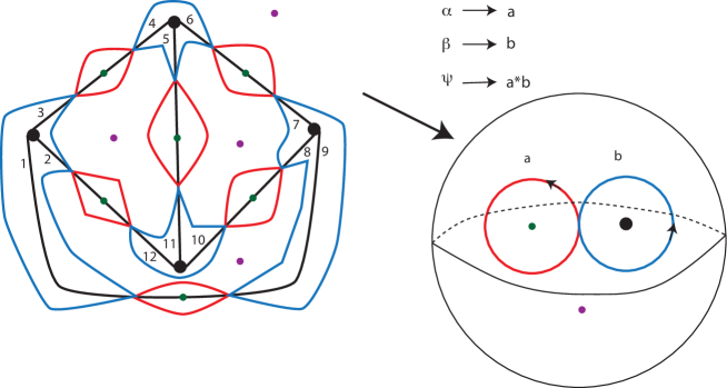
We are interested in branched coverings of the 2-sphere $S^{2}$ branched along three points $x_{1},x_{2},x_{3}\in S^{2}$. These coverings are related to a cell decomposition of the 2-sphere consisting of one vertex $v$, two edges $a$ and $b$, and three disks $D_{1},D_{2},D_{3}$ oriented in such a way that $\partial D_{1}=a,\partial D_{2}=b,\partial D_{3}=(a*b)^{-1}$. We regard $x_{i}$ as the center of $D_{i}$ (see Figure 1).

The fundamental group of the punctured 2-sphere is free of rank two and admits a presentation $\pi_{1}(S^{2}-\{x_{1},x_{2},x_{3}\})\cong\langle\bar{x}_{1},\bar{x}_{2},\bar{x}_{3}:\bar{x}_{1}\bar{x}_{2}\bar{x}_{3}=1\rangle$, where the symbol $\bar{x}_{i}$ is the class of a closed curve on $S^{2}$ starting at the vertex $v$ and encircling the point $x_{i}$. Alternatively, using the cell decomposition of $S^{2}$ above, we obtain a presentation $\pi_{1}(S^{2}-\{x_{1},x_{2},x_{3}\})\cong\langle a,b,c:abc=1\rangle$ where $a\simeq\bar{x}_{1}$, $b\simeq\bar{x}_{2}$, and $c=(a*b)^{-1}\simeq\bar{x}_{3}$. Therefore an $d$-fold branched covering of $S^{2}$ branched along $\{x_{1},x_{2},x_{3}\}$ is determined by a triple of permutations $\alpha,\beta,\gamma\in\Sigma_{d}$, such that $\alpha\beta\gamma=1$. The triple $(\alpha,\beta,\gamma)$ is called a constellation in [9]. An arbitrary pair of permutations $\alpha,\beta\in\Sigma_{d}$ gives a constellation, $(\alpha,\beta,\gamma)$, setting $\gamma=(\alpha\beta)^{-1}$.

A constellation $\alpha,\beta,\gamma\in\Sigma_{d}$ defines a representation $\omega:\pi_{1}(S^{2}-\{x_{1},x_{2},x_{3}\})\rightarrow\Sigma_{d}$ such that $\omega(a)=\alpha$, $\omega(b)=\beta$, and $\omega(c)=\gamma$. The associated branched covering $\varphi_{\omega}:F\rightarrow S^{2}$ can be constructed in two steps. First, construct the covering space of $a\vee b$ induced by the restriction $\omega:\pi_{1}(a\vee b)\rightarrow\Sigma_{d}$, and, secondly, construct the branched coverings of the disks $D_{i}$ branched along $x_{i}$ associated to the restrictions $\omega:\pi_{1}(D_{i}-\{x_{i}\})\rightarrow\Sigma_{d}$. These covers have as many components as the number of cycles in a disjoint cycle decomposition of $\omega(\partial(D_{i}))$. Finally assemble together these coverings into $F$ with liftings of the glueing maps $\partial D_{i}\rightarrow a\vee b$.

The $d$-fold branched cover $\phi:F\rightarrow S^{2}$ gets a cell decomposition for $F$ induced by the cell decomposition of $S^{2}$, with vertices $\varphi^{-1}(v)$, edges $\varphi^{-1}(a\cup b)$, and 2-cells $\varphi^{-1}(D_{1}\cup D_{2}\cup D_{3})$.

In this section we describe an algorithm to calculate the orientable genera of a graph $G$. For a set $Y$, we write $\Sigma(Y)$ for the symmetric group in the symbols in $Y$. If $\#(Y)=k$, we write $\Sigma_{k}=\Sigma(Y)$. If $\gamma\in\Sigma_{k}$, $|\gamma|$ is the number of cycles in a decomposition of $\gamma$ into disjoint cycles in $\Sigma_{k}$ (including trivial cycles for the fixed points of $\gamma$).

In this Section, we apply the algorithm to $K_{4}$, the complete graph of $4$ vertices as in Figure 2.

From Figure 2, we obtain the permutation $\alpha=(1,9)(2,12)(3,4)(5,11)(6,7)(8,10)$. We choose, as in the figure, $\beta=(1,2,3)(4,5,6)(7,8,9)(10,11,12)$, and then $\gamma=(\alpha\beta)^{-1}=(1,4,7)(2,9,10)(3,12,5)(6,11,8)$. Here $e=6$, $t_{j}=3$ for $j=1,2,3,4$, and $l_{k}=3$ for $k=1,2,3,4$.

Using the Riemann-Hurwitz formula we obtain:

So, $\tilde{X}$ is the $2$-sphere. But we did know that $K_{4}$ is planar.

The graph $G^{\prime}$ looks like the graph in the left side of Figure 3, and in that figure one can see the corresponding branched cover of the 2-sphere.

Now $g_{M}(K_{4})=1$, and this genus can be achieved with the representation $\alpha=(1,9)(2,12)(3,4)(5,11)(6,7)(8,10)$ as before, but $\beta=(1,2,3)(4,5,6)(7,8,9)(10,12,11)$. Then $(\alpha\beta)^{-1}=(4,7,1)(10,5,3,12,8,6,11,2,9)$, and using the genus formula again we obtain:

In this section, we list the orientable genus and maximal orientable genus of some Snarks. Recall that a Snark is a 3-regular graph, which is 4-edge connected and it is not 3-edge-colourable. Many examples of Snarks are known, this is an interesting but mysterious class of graphs. We use the list of snarks and the notation given in [14]. A program for 3-regular graphs implementing the algorithm of Section 3, and written in the GAP programming language is available from the authors on request.

Acknowledgement. The first author is supported by a fellowship Investigadoras por México from CONAHCYT. Research partially supported by the grant PAPIIT-UNAM IN117423.

References

- [1] D. Archdeacon, A Kuratowski theorem for the projective plane. J. Graph Theory 5 (1981), 243-246.
- [2] I. Berstein and A. Edmonds, On the construction of branched coverings of low-dimensional manifolds. Trans. Amer. Math. Soc. 247 (1979), 87-124.
- [3] H. Djidjev and J. Reif, An efficient algorithm for the genus problem with explicit construction of forbidden subgraphs. Proc. of the 23rd. ACM Symp. theory of Comp., (1991), 337-347.
- [4] R.A. Duke, The genus, regional number, and Betti number of a graph. Canad. J. Math. 18, 817-822.
- [5] J.R. Edmonds, A combinatorial representation for polyhedral surfaces, American Mathematical Society Notices 7 (1960), 646.
- [6] I. S. Filotti, G. L. Miller and J. Reif, On determining the genus of a graph in steps. Proc. of the 11th ACM Symp. Theory of Comp., (1979), 27-37.
- [7] J. L. Gross, Embeddings of graphs of fixed treewidth and bounded degree. ARS Mathematica Contemporanea 7 (2014), 379-403.
- [8] K. Kawarabayashi, B. Mohar and B. Reed, A simpler linear time algorithm for embedding graphs into an arbitrary surface and the genus of graphs of bounded treewidth. Proc. 49th Ann. Symp. on Foundations of Computer Science (FOCS’08) IEEE (2008), 771-780.
- [9] S. K. Lando and A. K. Zvonkin, Graphs on Surfaces and their Applications. Encyclopaedia of Mathematical Sciences Vol. 141, Springer-Verlag, 2004.
- [10] B. Mohar, Embedding graphs in an arbitrary surface in linear time. Proc. 28th Ann. ACM STOC, Philadelphia, ACM Press, 1996, pp. 392-397.
- [11] B. Mohar, A linear time algorithm for embedding graphs in an arbitrary surface. SIAM J. Discrete Math 12 (1999), 6-26.
- [12] W. Myrvold and W. Kocay, Errors in graph embedding algorithms. Journal of Computer and System Sciences 77 (2011), 430-438.
- [13] B. Mohar and C. Thomassen, Graphs on Surfaces. Johns Hopkins University Press, Baltimore, MD, 2001.
- [14] R. C. Read, R. J. Wilson, An Atlas of Graphs. Oxford Science Publications, 2005.
- [15] G. Ringel. Map Color Theorem, Die Grundlehren der mathematischen Wissenschaften 209 Berlin-Heidelberg-New York: Springer-Verlag XII, 191 pp. 1974.
- [16] S. Stahl, The embedding of s graph - a survey. Journal of Graph Theory 2 (1978), 275–298.
- [17] C. Thomassen, The graph genus problem is NP-complete. J. Algorithms 10 (1989), 568-576.
- [18] J.W.T. Youngs, Minimal imbeddings and the genus of a graph. J. Math. Mech. 12 (1963), 303–315