Generic transverse stability of kink structures in atomic and optical nonlinear media with competing attractive and repulsive interactions
Abstract
We demonstrate the existence and stability of one-dimensional (1D) topological kink configurations immersed in higher-dimensional bosonic gases and nonlinear optical setups. Our analysis pertains, in particular, to the two- and three-dimensional extended Gross-Pitaevskii models with quantum fluctuations describing droplet-bearing environments but also to the two-dimensional cubic-quintic nonlinear Schrödinger equation containing higher-order corrections to the nonlinear refractive index. Contrary to the generic dark soliton transverse instability, the kink structures are generically robust under the interplay of low-amplitude attractive and high-amplitude repulsive interactions. A quasi-1D effective potential picture dictates the existence of these defects, while their stability is obtained through linearization analysis and direct dynamics in the presence of external fluctuations showcasing their unprecedented resilience. These generic (across different models) findings should be detectable in current cold atom and optics experiments. They also offer insights towards controlling topological excitations and their usage in topological quantum computers.
Introduction.
Kink solitons (alias domain walls) are nonlinear excitations encountered in disparate disciplines ranging from optical Kartashov et al. (2006), and magnetic media Pérez-Junquera et al. (2008); Buijnsters et al. (2014), living cellular structures Ivancevic and Ivancevic (2013); Yomosa (1983); Caspi and Ben-Jacob (1999), folding protein chains Hu et al. (2011a, b) to atomic gases Tylutki et al. (2020); Katsimiga et al. (2023a) and cosmology Vilenkin and Shellard (2000). Their topological character has been recently unveiled in two-dimensional (2D) van der Waals materials Lee et al. (2023), opening up the possibility of robust computations Wang et al. (2022). Stabilization of multidimensional spatially localized states is a fundamental challenge of scientific interest in physics and beyond Kartashov et al. (2019). It is well-known that 1D topological (e.g. dark solitons) and non-topological (bright solitons) defects suffer from the so-called snake-instability Tikhonenko et al. (1996); Mamaev et al. (1996); Kivshar and Pelinovsky (2000); Anderson et al. (2001) and infrared catastrophe Bergé (1998); Fibich (2015), respectively, once embedded in 2D and three-dimensional (3D) geometries. Mechanisms of suppression of the ensuing instabilities of defects have also been discussed. These mainly consider nonuniform media, i.e., incorporating external trapping geometries Proukakis et al. (2004); Wen et al. (2013); Kevrekidis et al. (2004), or are accompanied by nonlocal interactions Skupin et al. (2006); Lin et al. (2008); Nath et al. (2008), or accounting for the active competition of higher-order nonlinearities Zeng and Zeng (2020).
Cold atoms are ideal quantum many-body simulators, i.e., platforms featuring remarkable tunability of system parameters, such as e.g. interactions and external traps Bloch et al. (2008); Lewenstein et al. (2012). In this context, ultradilute and incompressible self-bound states of matter, referred to as quantum droplets Luo et al. (2021); Mistakidis et al. (2023) were recently experimentally detected in Bose mixtures Cheiney et al. (2018); Semeghini et al. (2018); Cabrera et al. (2018); D’Errico et al. (2019); Burchianti et al. (2020) and dipolar gases Chomaz et al. (2023); Böttcher et al. (2020). Stabilization of these states is achieved through the counterbalance of attractive and repulsive interactions modeled by mean-field nonlinear couplings and quantum fluctuations. The latter are incorporated perturbatively through the famous Lee-Huang-Yang (LHY) Lee et al. (1957); Larsen (1963) correction whose sign and form depend on dimensionality Ilg et al. (2018) leading to an extended Gross-Pitaevskii equation (eGPE) Petrov (2015); Petrov and Astrakharchik (2016). Such environments sustain also different kinds of nonlinear excitations such as dark solitons Edmonds (2023); Katsimiga et al. (2023b); Saqlain et al. (2023), bubbles Katsimiga et al. (2023a); Edmonds (2023), kinks Kartashov et al. (2022); Tylutki et al. (2020); Katsimiga et al. (2023a) and vortices Li et al. (2018); Yoğurt et al. (2023).
From a complementary nonlinear optics-seeded perspective, the Cubic-Quintic (CQ) model is an extension of the famous nonlinear Schrödinger model Killip et al. (2017) constituing a universal mathematical toolbox involving higher-order nonlinearities. In the optical setting, CQ is utilized to study the propagation of electromagnetic waves Falcão Filho et al. (2013); Reyna et al. (2020) in photorefractive materials. In this context, the quintic term accounts for higher-order corrections to the nonlinear refractive index Akhmediev and Afanasjev (1995), i.e., incorporating susceptibilities up to fifth-order. Experimentally, it is often also relevant to include the nontrivial (dissipative) absorption effects. The broad applicability of CQ manifests by the fact that it has been deployed to describe various phenomena, for instance, liquid waveguides Falcão Filho et al. (2013), special types of glasses Boudebs et al. (2003), and colloids containing metallic nanoparticles Falcão-Filho et al. (2007). In atomic gases, the cubic (quintic) coupling is related to the two- (three-) body interactions Luckins and Van Gorder (2018); Cardoso et al. (2011); Bulgac (2002) (see also, e.g., Kolomeisky et al. (2000)).
In this Letter we explore the dynamical transverse stability of kinks in a wide range of models from nonlinear optics and atomic physics, such as the 2D and 3D eGPE settings, as well as the 2D CQ model. A key feature of these setups is the competition between attractive nonlinearities (dominant at low density) and repulsive ones (prevailing at high density) whose presence is proved crucial for the stability of kinks. Specifically, the stability and robustness of these entities is demonstrated in a twofold manner. Firstly, we analytically extract and numerically evaluate the relevant for each model Bogoliubov-de-Gennes (BdG) spectrum. Secondly, we subject the relevant one-dimensional (1D) kink solutions to external, spatially distributed fluctuations (customarily present in experimental settings) and subsequently monitor their remarkable persistence for evolution times of the order of seconds. This demonstrates the relevance of these 1D topological defects in current state-of-the-art cold atom and nonlinear optics experiments and their structural robustness as potential information carriers.
Models and Theoretical Analysis.
To highlight the universal features of the existence and stability of kink solutions in higher spatial dimensions, three different nonlinear models characterized by competing attractive (at low density) and repulsive (at high density) interactions are investigated. These correspond to the eGPEs describing, for instance, self-bound quantum droplets in 2D Petrov and Astrakharchik (2016); Luo et al. (2021) and 3D Petrov (2015); Luo et al. (2021), and the CQ equation. Experimentally, the droplet bearing systems can be emulated e.g. by considering two hyperfine states of 39K Semeghini et al. (2018). In optics the CQ model is typically used to monitor, for instance, optical beam profiles of topological defects in liquid Reyna et al. (2020). In dimensionless form (see also supplemental material (SM) sup ) these equations read
| (1a) | |||
| (1b) | |||
| (1c) | |||
Here, Eqs. (1a) and (1c) refer to the 2D and 3D eGPEs, while Eq. (1b) is the 2D CQ model with . In the 2D eGPE, the logarithmic nonlinearity encompasses both mean-field and first-order quantum fluctuation effects Petrov and Astrakharchik (2016); Luo et al. (2021), while its 3D counterpart features a cubic (resp. quartic) attractive with (resp. repulsive) mean-field (LHY) contribution Petrov (2015), see also SM sup . Furthermore, in the CQ model there is an attractive (repulsive) cubic (quintic) nonlinear coupling commonly accounting for two- (three-) body interactions in the realm of cold gases Luckins and Van Gorder (2018); Bulgac (2002) or higher order corrections to the Kerr effect in nonlinear optics Akhmediev and Afanasjev (1995); Reyna et al. (2020).
To infer the existence of planar kinks (i.e., one dimensional ones embedded in higher dimensions), the following ansatz is employed, . Here, denotes the chemical potential and () are the transverse coordinates of the wave function in 2D (3D). A uniform background is assumed along the transverse directions, and the waveform is taken to be real without loss of generality. Introducing this ansatz into Eqs. (1a)-(1c) results in their reduced effective 1D time-independent standing wave analogues. These can be cast into Newtonian equations of motion, , subjected to the relevant for each model effective potential . These turn out to be
| (2a) | |||
| (2b) | |||
| (2c) | |||
Integration of the Newtonian equations of motion yields the effective energy, , of the 1D reduced system Katsimiga et al. (2023b). While the resulting potentials feature multiple maxima, the frequency parameter can be generically tuned to render these maxima equi-energetic, thus enabling a genuine heteroclinic orbit, i.e., a kink, between and with .
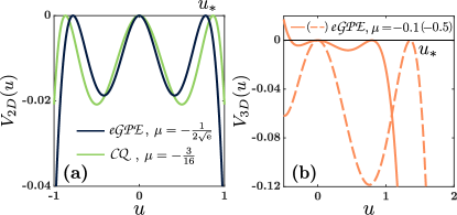
To systematically determine the finite kink backgrounds and chemical potentials, two conditions need to be satisfied, and , namely, conditions for the maximum at being equi-energetic with the one at . For the 2D eGPE (CQ) these values lead analytically to , ( and ) [Fig. 1(a)]. The boundary for the 2D eGPE separates the parameter region of 2D droplets from that of 2D bubbles Luo et al. (2021); Petrov and Astrakharchik (2016), analogously to what is the case also in 1D Katsimiga et al. (2023a). For the 3D eGPE, the chemical potential and extremum are and respectively [Fig. 1(b)]. Notice that while such kink-type states have been discussed for CQ settings previously (see, e.g., Jin-Liang et al. (2006)), they are unprecedented, to our knowledge, for the emergent atomic theme of 2D and 3D quantum droplet settings. Interestingly, the asymmetry of the effective potential [Fig. 1(b)] suggests the concurrent existence of a heretofore unexplored quantum droplet (for values of ) whose analysis is deferred for future studies.
Within the effective potential framework, unique kink solutions exist for each coupling strength when competing interactions exist, i.e., when . In what follows, without loss of generality and are set to unity in order to inspect the stability properties of these topological defects. On the other hand, the mean-field interaction in the 3D eGPE is routinely tunable in experiments via Feshbach resonances, see Semeghini et al. (2018) and SM sup .
Spectral stability of kinks in higher dimensions.
According to the aforementioned effective potential description the 1D planar kink solution occurs for , , and e.g. where , within the 2D eGPE, 2D CQ and 3D eGPE model, respectively. The relevant effective 1D but also the higher dimensional stationary states are then obtained upon utilizing heteroclinic (tanh-shaped) initial guesses, bearing the correct asymptotics described above. In the CQ case, an analytical form exists as Jin-Liang et al. (2006); Birnbaum and Malomed (2008). It is then numerically confirmed that such 1D planar waveforms satisfy the corresponding 2D and 3D time-independent version of Eqs. (1a)-(1c).
Then, in order to extract the stability properties of these configurations, small perturbations of the numerically exact (up to a prescribed tolerance) kink solutions are considered having the form . Here, denotes complex conjugation, and refer to the corresponding eigenvectors, and eigenfrequencies, whilst is a small perturbation parameter. Utilizing the above wave function ansatz and keeping terms of order one arrives at an eigenvalue problem that, irrespectively of the system under consideration [Eqs. (1a)-(1c)], can be written as
| (3) |
The model-dependent diagonal matrix elements are found to be , , and , for the 2D eGPE, CQ, and 3D eGPE respectively. Their relevant off-diagonal counterparts read , , and , respectively. In all cases, , and denotes the -dimensional Laplace operator. Additionally, designates the stationary, real kink state for each distinct model.
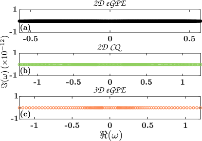
The stability analysis outcome for all three models investigated herein, is depicted in Figs. 2(a)-(c). In all scenarios, spectral stability of the kink state can be inferred from the absence of a finite imaginary part, , in the pertinent BdG spectrum. For all settings, the first hundred eigenvalues of the continuous quasi-1D BdG spectra are illustrated, while we note that we verified that their relevant higher dimensional analogues produce the same stability result. By quasi-1D BdG spectra, what is meant here is that the transverse direction is decomposed into Fourier modes (with the “quantization” thereof from a finite transverse computational domain accounted for) and the stability of (a large number of) effective 1D spectra for different transverse wavenumbers is confirmed.
Dynamical confirmation of the absence of transverse instability for the kinks.
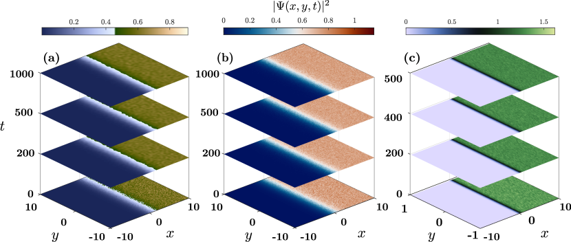
To corroborate our BdG findings we next consider the dynamical evolution of the stationary kink solution for each of the models under study. Specifically, we aim not only to mimic unavoidable experimental imperfections but also to exemplify the robust nature of the kink structure in the presence of transverse perturbations. To that effect, the kink initial state is significantly perturbed via a random normal distribution generator, . The ensuing wave function acquires the form . In this context, is characterized by zero mean and unit variance, while such that also phase disturbances are encountered. In particular, the considered amplitudes of the perturbation range lie in the interval of the solution amplitude. Typical evolution times (in the dimensionless units adopted herein) are of the order of and for the 3D and 2D settings, respectively, confirming the longevity of these planar 1D defects upon their exposure to transverse excitations.
Evidently, despite the significantly excited nature of the initial state the kink remains intact preserving its shape throughout the evolution, while “shedding” some of the relevant “radiation” in the form of dispersive wavepackets, as it can be seen in Figs. 3(a)-(c). Particularly here, distinct plates correspond to density, , contours in the plane taken at different times during the propagation of the perturbed kink configuration. For the 3D dynamics the -direction is integrated out, while we note that the robustness of the kink configurations has also been verified for different values of the chemical potential and hence distinct interaction strengths.
Experimental implications.
A binary bosonic mixture in the ultracold regime, where interspecies attraction is balanced by intraspecies repulsion, can host self-bound states Petrov (2015); Cheiney et al. (2018); Semeghini et al. (2018). The two hyperfine levels , of 39K in the vicinity of the intraspecies Feshbach resonance Chin et al. (2010); D’Errico et al. (2007) were proven to be suitable candidates satisfying the above criteria Cabrera et al. (2018); Semeghini et al. (2018). These two states are experimentally populated using radiofrequency spectroscopy Cabrera et al. (2018) and their dynamics can be adequately described by the eGPE models [Eqs. (1a), (1c)] in 2D and 3D. For such a setup with averaged mean-field scattering length , the propagation times of the kink defect in 3D ( in dimensionless units) refer approximately to sup . A corresponding pancake geometry confining such a 2D mixture can be realized by utilizing a tight harmonic trap along one spatial dimension Hadzibabic and Dalibard (2011). For an experimentally relevant trapping frequency Cabrera et al. (2018); Saint-Jalm et al. (2019) and [see SM sup ], the relevant timescale ( in dimensionless units) for the kink evolution is secs. These long evolution times guarantee the resilience of the kink structure for its realization in current state-of-the-art experiments that suffer in addition by three-body recombination processes Semeghini et al. (2018).
On the other hand, the 2D CQ equation is used to describe, for instance, the propagation of electromagnetic waves in optical media incorporating higher-order nonlinear refractive indices Sutherland (2003). Characteristic materials featuring such properties are chalcogenide glasses Boudebs et al. (2003), such as liquid Falcão Filho et al. (2013); Reyna et al. (2020). In such setups (where optical vortices and their destabilization has been monitored Desyatnikov et al. (2005)), the time-evolution can be probed by measuring the transmission of the kink along the axial direction of the nonlinear medium. Considering a light beam of Falcão Filho et al. (2013), a propagation distance of corresponds to axial depth for the kink transmission. In the above-discussed setups, namely either cold bosonic mixtures or nonlinear optical media, kink defects can be imprinted in the bulk by means of the well-established technique of phase masking Denschlag et al. (2000); Pedaci et al. (2006) or utilizing digital micromirror device patterned optical traps Saint-Jalm et al. (2019); Navon et al. (2021); Gauthier et al. (2016).
Conclusions and future challenges.
The existence and corresponding spectral and dynamical stability of 1D kink solutions embedded in higher-dimensional gases or nonlinear optical media featuring competing attractive lower order and repulsive higher order interactions is unveiled. This is exemplarily demonstrated for three distinct, representative models referring to the 2D and 3D eGPE droplet bearing systems and the 2D CQ setting relevant in nonlinear optics, in order to establish the breadth and generality of results. We explicated the existence of these 1D topological defects upon analytically extracting, in each case, a quasi-1D effective potential picture, subsequently supplemented by their spectral stability inferred through linearization analysis. Additionally, monitoring their dynamical evolution in the presence of external fluctuations, with amplitudes up to 50% of the actual solution, revealed their profound robustness and resilience, for times up to few seconds.
These results suggest the use of kink defects as promising candidates for topological quantum computing. Indeed, contrary to the generically (in such nonlinear Schrödinger models) transversely unstable dark soliton states, which have been studied and reviewed extensively Kivshar and Pelinovsky (2000), kinks appear to defy the proneness to transverse modulations. Importantly, also, these results pave the way for significant further both physical and mathematical studies. On the latter side, a rigorous proof of such stability is a key open direction. On the other hand, from a physical perspective, our effective potential analysis suggests the existence of further lower-dimensional nonlinear excitations (including droplets, bubbles, etc.), whose transverse dynamics and potential dynamical features may be of further theoretical and experimental interest in its own right. Such studies are currently in progress and will be reported in future publications.
Acknowledgments.
We acknowledge fruitful discussions with B. Malomed. This material is based upon work supported by the U.S. National Science Foundation under the awards PHY-2110030 and DMS-2204702 (PGK).
References
- Kartashov et al. (2006) Y. V. Kartashov, V. A. Vysloukh, and L. Torner, Opt. Express 14, 12365 (2006).
- Pérez-Junquera et al. (2008) A. Pérez-Junquera, V. Marconi, A. B. Kolton, L. Álvarez-Prado, Y. Souche, A. Alija, M. Vélez, J. V. Anguita, J. Alameda, J. I. Martín, and J. M. R. Parrondo, Phys. Rev. Lett. 100, 037203 (2008).
- Buijnsters et al. (2014) F. J. Buijnsters, A. Fasolino, and M. I. Katsnelson, Phys. Rev. Lett. 113, 217202 (2014).
- Ivancevic and Ivancevic (2013) V. G. Ivancevic and T. T. Ivancevic, J. Geom. Symmetry Phys. 31, 1 (2013).
- Yomosa (1983) S. Yomosa, Phys. Rev. A 27, 2120 (1983).
- Caspi and Ben-Jacob (1999) S. Caspi and E. Ben-Jacob, Europhys. Lett. 47, 522 (1999).
- Hu et al. (2011a) S. Hu, M. Lundgren, and A. J. Niemi, Phys. Rev. E 83, 061908 (2011a).
- Hu et al. (2011b) S. Hu, A. Krokhotin, A. J. Niemi, and X. Peng, Phys. Rev. E 83, 041907 (2011b).
- Tylutki et al. (2020) M. Tylutki, G. E. Astrakharchik, B. A. Malomed, and D. S. Petrov, Phys. Rev. A 101, 051601(R) (2020).
- Katsimiga et al. (2023a) G. C. Katsimiga, S. I. Mistakidis, B. A. Malomed, D. J. Frantzeskakis, R. Carretero-Gonzalez, and P. G. Kevrekidis, Condensed Matter 8, 67 (2023a).
- Vilenkin and Shellard (2000) A. Vilenkin and E. P. S. Shellard, Cosmic Strings and Other Topological Defects (Cambridge University Press, 2000).
- Lee et al. (2023) J. Lee, J. W. Park, G. Y. Cho, and H. W. Yeom, Adv. Mat. 35, 2300160 (2023).
- Wang et al. (2022) I.-T. Wang, C.-C. Chang, Y.-Y. Chen, Y.-S. Su, and T.-H. Hou, Neuromorph. Comput. Eng. 2, 012003 (2022).
- Kartashov et al. (2019) Y. V. Kartashov, G. E. Astrakharchik, B. A. Malomed, and L. Torner, Nat. Rev. Phys. 1, 185 (2019).
- Tikhonenko et al. (1996) V. Tikhonenko, J. Christou, B. Luther-Davies, and Y. S. Kivshar, Opt. Lett. 21, 1129 (1996).
- Mamaev et al. (1996) A. Mamaev, M. Saffman, and A. Zozulya, Phys. Rev. Lett. 76, 2262 (1996).
- Kivshar and Pelinovsky (2000) Y. S. Kivshar and D. E. Pelinovsky, Phys. Rep. 331, 117 (2000).
- Anderson et al. (2001) B. Anderson, P. Haljan, C. Regal, D. Feder, L. Collins, C. W. Clark, and E. A. Cornell, Phys. Rev. Lett. 86, 2926 (2001).
- Bergé (1998) L. Bergé, Phys. Rep. 303, 259 (1998).
- Fibich (2015) G. Fibich, The nonlinear Schrödinger equation, Vol. 192 (Springer, 2015).
- Proukakis et al. (2004) N. Proukakis, N. Parker, D. Frantzeskakis, and C. Adams, J. Opt. B: Quantum Semiclass. Opt. 6, S380 (2004).
- Wen et al. (2013) W. Wen, C. Zhao, and X. Ma, Phys. Rev. A 88, 063621 (2013).
- Kevrekidis et al. (2004) P. G. Kevrekidis, G. Theocharis, D. J. Frantzeskakis, and A. Trombettoni, Phys. Rev. A 70, 023602 (2004).
- Skupin et al. (2006) S. Skupin, O. Bang, D. Edmundson, and W. Krolikowski, Phys. Rev. E 73, 066603 (2006).
- Lin et al. (2008) Y. Lin, R.-K. Lee, and Y. S. Kivshar, J. Opt. Soc. Am. B 25, 576 (2008).
- Nath et al. (2008) R. Nath, P. Pedri, and L. Santos, Phys. Rev. Lett. 101, 210402 (2008).
- Zeng and Zeng (2020) L. Zeng and J. Zeng, Commun. Phys. 3, 26 (2020).
- Bloch et al. (2008) I. Bloch, J. Dalibard, and W. Zwerger, Rev. Mod. Phys. 80, 885 (2008).
- Lewenstein et al. (2012) M. Lewenstein, A. Sanpera, and V. Ahufinger, Ultracold Atoms in Optical Lattices: Simulating quantum many-body systems (OUP Oxford, 2012).
- Luo et al. (2021) Z.-H. Luo, W. Pang, B. Liu, Y.-Y. Li, and B. A. Malomed, Front. Phys. 16, 1 (2021).
- Mistakidis et al. (2023) S. I. Mistakidis, A. G. Volosniev, R. E. Barfknecht, T. Fogarty, T. Busch, A. Foerster, P. Schmelcher, and N. T. Zinner, Phys. Rep. 1042, 1 (2023).
- Cheiney et al. (2018) P. Cheiney, C. R. Cabrera, J. Sanz, B. Naylor, L. Tanzi, and L. Tarruell, Phys. Rev. Lett. 120, 135301 (2018).
- Semeghini et al. (2018) G. Semeghini, G. Ferioli, L. Masi, C. Mazzinghi, L. Wolswijk, F. Minardi, M. Modugno, G. Modugno, M. Inguscio, and M. Fattori, Phys. Rev. Lett. 120, 235301 (2018).
- Cabrera et al. (2018) C. R. Cabrera, L. Tanzi, J. Sanz, B. Naylor, P. Thomas, P. Cheiney, and L. Tarruell, Science 359, 301 (2018).
- D’Errico et al. (2019) C. D’Errico, A. Burchianti, M. Prevedelli, L. Salasnich, F. Ancilotto, M. Modugno, F. Minardi, and C. Fort, Phys. Rev. Research 1, 033155 (2019).
- Burchianti et al. (2020) A. Burchianti, C. D’Errico, M. Prevedelli, L. Salasnich, F. Ancilotto, M. Modugno, F. Minardi, and C. Fort, Cond. Matt. 5, 21 (2020).
- Chomaz et al. (2023) L. Chomaz, I. Ferrier-Barbut, F. Ferlaino, B. Laburthe-Tolra, B. L. Lev, and T. Pfau, Rep. Progr. Phys. 86, 026401 (2023).
- Böttcher et al. (2020) F. Böttcher, J.-N. Schmidt, J. Hertkorn, K. S. H. N g, S. D. Graham, M. Guo, T. Langen, and T. Pfau, Rep. Progr. Phys. 84, 012403 (2020).
- Lee et al. (1957) T. D. Lee, K. Huang, and C. N. Yang, Phys. Rev. 106, 1135 (1957).
- Larsen (1963) D. M. Larsen, Ann. Phys. (New York)(US) 24 (1963).
- Ilg et al. (2018) T. Ilg, J. Kumlin, L. Santos, D. S. Petrov, and H. P. Büchler, Phys. Rev. A 98, 051604 (2018).
- Petrov (2015) D. S. Petrov, Phys. Rev. Lett. 115, 155302 (2015).
- Petrov and Astrakharchik (2016) D. S. Petrov and G. E. Astrakharchik, Phys. Rev. Lett. 117, 100401 (2016).
- Edmonds (2023) M. Edmonds, Phys. Rev. Research 5, 023175 (2023).
- Katsimiga et al. (2023b) G. C. Katsimiga, S. I. Mistakidis, G. N. Koutsokostas, D. J. Frantzeskakis, R. Carretero-González, and P. G. Kevrekidis, Phys. Rev. A 107, 063308 (2023b).
- Saqlain et al. (2023) S. Saqlain, T. Mithun, R. Carretero-González, and P. G. Kevrekidis, Phys. Rev. A 107, 033310 (2023).
- Kartashov et al. (2022) Y. V. Kartashov, V. M. Lashkin, M. Modugno, and L. Torner, New J. Phys. 24, 073012 (2022).
- Li et al. (2018) Y. Li, Z. Chen, Z. Luo, C. Huang, H. Tan, W. Pang, and B. A. Malomed, Phys. Rev. A 98, 063602 (2018).
- Yoğurt et al. (2023) T. A. Yoğurt, U. Tanyeri, A. Keleş, and M. Oktel, Phys. Rev. A 108, 033315 (2023).
- Killip et al. (2017) R. Killip, T. Oh, O. Pocovnicu, and M. Vişan, Archive for Rational Mechanics and Analysis 225, 469 (2017).
- Falcão Filho et al. (2013) E. L. Falcão Filho, C. B. de Araújo, G. Boudebs, H. Leblond, and V. Skarka, Phys. Rev. Lett. 110, 013901 (2013).
- Reyna et al. (2020) A. S. Reyna, H. T. M. C. M. Baltar, E. Bergmann, A. M. Amaral, E. L. Falcão Filho, P.-F. m. c. Brevet, B. A. Malomed, and C. B. de Araújo, Phys. Rev. A 102, 033523 (2020).
- Akhmediev and Afanasjev (1995) N. Akhmediev and V. Afanasjev, Phys. Rev. Lett. 75, 2320 (1995).
- Boudebs et al. (2003) G. Boudebs, S. Cherukulappurath, H. Leblond, J. Troles, F. Smektala, and F. Sanchez, Opt. Comm. 219, 427 (2003).
- Falcão-Filho et al. (2007) E. Falcão-Filho, C. B. de Araújo, and J. Rodrigues Jr, JOSA B 24, 2948 (2007).
- Luckins and Van Gorder (2018) E. K. Luckins and R. A. Van Gorder, Ann. Phys. 388, 206 (2018).
- Cardoso et al. (2011) W. B. Cardoso, A. T. Avelar, and D. Bazeia, Phys. Rev. E 83, 036604 (2011).
- Bulgac (2002) A. Bulgac, Phys. Rev. Lett. 89, 050402 (2002).
- Kolomeisky et al. (2000) E. B. Kolomeisky, T. J. Newman, J. P. Straley, and X. Qi, Phys. Rev. Lett. 85, 1146 (2000).
- (60) In the Supplementary Material more information can be found regarding the dimensionful expressions of the nonlinear models, as well as the relation with physical parameters.
- Jin-Liang et al. (2006) Z. Jin-Liang, W. Ming-Liang, and L. Xiang-Zheng, Commun. Theor. Phys. 45, 343 (2006).
- Birnbaum and Malomed (2008) Z. Birnbaum and B. A. Malomed, Physica D: Nonlinear Phenomena 237, 3252 (2008).
- Chin et al. (2010) C. Chin, R. Grimm, P. Julienne, and E. Tiesinga, Rev. Mod. Phys. 82, 1225 (2010).
- D’Errico et al. (2007) C. D’Errico, M. Zaccanti, M. Fattori, G. Roati, M. Inguscio, G. Modugno, and A. Simoni, New J. Phys. 9, 223 (2007).
- Hadzibabic and Dalibard (2011) Z. Hadzibabic and J. Dalibard, La Rivista del Nuovo Cimento 34, 389 (2011).
- Saint-Jalm et al. (2019) R. Saint-Jalm, P. C. M. Castilho, E. Le Cerf, B. Bakkali-Hassani, J.-L. Ville, S. Nascimbene, J. Beugnon, and J. Dalibard, Phys. Rev. X 9, 021035 (2019).
- Sutherland (2003) R. L. Sutherland, Handbook of nonlinear optics (CRC press, 2003).
- Desyatnikov et al. (2005) A. S. Desyatnikov, Y. S. Kivshar, and L. Torner, in Progr. Opt., Vol. 47 (2005) pp. 291–391.
- Denschlag et al. (2000) J. Denschlag, J. E. Simsarian, D. L. Feder, C. W. Clark, L. A. Collins, J. Cubizolles, L. Deng, E. W. Hagley, K. Helmerson, W. P. Reinhardt, and S. L. Rolston, Science 287, 97 (2000).
- Pedaci et al. (2006) F. Pedaci, P. Genevet, S. Barland, M. Giudici, and J. Tredicce, Appl. Phys. Lett. 89 (2006).
- Navon et al. (2021) N. Navon, R. P. Smith, and Z. Hadzibabic, Nat. Phys. 17, 1334 (2021).
- Gauthier et al. (2016) G. Gauthier, I. Lenton, N. M. Parry, M. Baker, M. Davis, H. Rubinsztein-Dunlop, and T. Neely, Optica 3, 1136 (2016).
- Otajonov et al. (2020) S. R. Otajonov, E. N. Tsoy, and F. K. Abdullaev, Phys. Rev. E 102, 062217 (2020).
- Abramowitz et al. (1988) M. Abramowitz, I. A. Stegun, and R. H. Romer, “Handbook of mathematical functions with formulas, graphs, and mathematical tables,” (1988).
- Petrov and Shlyapnikov (2001) D. S. Petrov and G. V. Shlyapnikov, Phys. Rev. A 64, 012706 (2001).
- Petrov et al. (2000) D. S. Petrov, M. Holzmann, and G. V. Shlyapnikov, Phys. Rev. Lett. 84, 2551 (2000).
Supplementary Material:
Generic transverse stability of kink structures in atomic and optical nonlinear media with competing repulsive and attractive interactions
I Three-dimensional attractive mixture
The three-dimensional setting discussed in the main text corresponds to an attractive bosonic mixture, where the intercomponent attraction slightly exceeds the intracomponent repulsion. Namely, , with denoting the relevant 3D scattering lengths that are tunable with the Feshbach resonance technique Semeghini et al. (2018). In this interaction regime, it is theoretically predicted Petrov (2015); Luo et al. (2021) and experimentally observed Cabrera et al. (2018); Semeghini et al. (2018) that the bosonic mixture hosts many-body self-bound states, known as quantum droplets. The beyond mean-field first-order LHY correction is proven to be crucial for sustaining such structures, minimizing the underlying energy functional of the mixture. The resulting extended mean-field equations (eGPEs) then feature competing nonlinearities, expressed through a cubic and a quartic term Petrov (2015).
When the ratio between the density of the components satisfies , the two coupled extended mean-field equations reduce to a single effective one Semeghini et al. (2018), describing an attractive bosonic mixture. The dimensional form of the eGPE reads Semeghini et al. (2018)
| (S1) |
Here, is the mass of the atoms, is the 3D wave function describing the reduced single component, and the averaged mean-field interactions .
To render Eq. (S1) dimensionless, the following transformations are employed,
| (S2) |
where e.g. is the length of the box along the direction. With the above units, the 3D eGPE becomes dimensionless,
| (S3) |
The notation has been dropped for simplicity. Moreover, the dimensionless interaction strengths in these units read
| (S4a) | |||
| (S4b) | |||
Rescaling the wavefunction as , we absorb the prefactor in front of the quartic term and we recover Eq. (1c) in the main text. For the two hyperfine states of 39K Semeghini et al. (2018); Cabrera et al. (2018); Cheiney et al. (2018), it was shown that droplets can form when is tuned to small negative values by means of Fano-Feshbach resonances Chin et al. (2010). Relevant timescales correspond to .
II Two-dimensional droplet setting
Here, we elaborate on the 2D eGPE supporting quantum droplets, its dimensionless form, and the connection of the interaction strengths with the experimentally tunable 3D scattering lengths. Quantum droplets can also form in two dimensions Petrov and Astrakharchik (2016), where the logarithmic nonlinearity incorporates both the LHY term and the mean-field contributions. Similar to 3D, the corresponding coupled system of eGPEs can be reduced to an effective single-component one Otajonov et al. (2020), which reads
| (S5) |
The dimensionless interaction strength is related to the 2D scattering lengths through the expression Petrov and Astrakharchik (2016); Otajonov et al. (2020),
| (S6a) | |||
| (S6b) | |||
In these expressions, refer to the 2D scattering lengths within () or between () the components. Moreover, is the droplet equilibrium density in the thermodynamic limit Petrov and Astrakharchik (2016) and is the Euler-Mascheroni constant Abramowitz et al. (1988).
In the case of a tightly confined mixture in the -direction due to the presence of a harmonic trap with oscillator length , the scattering lengths are connected to their 3D counterparts, by Petrov and Shlyapnikov (2001); Petrov et al. (2000)
| (S7) |
Below, we measure time and length with respect to and respectively Saint-Jalm et al. (2019) and normalize the 2D wave function in terms of the total particle number, . In this sense the corresponding dimensionless eGPE is retrieved,
| (S8) |
III Cubic-quintic model
Below we elaborate on the dimensionalization of the cubic-quintic equation in the context of non-linear optical media discussed in the main text [Eq. (1b)]. Particularly, the relevant model considers light beams passing through nonlinear media, being characterized by high-order refractive index prefactors (stemming from an expansion of the refractive index as a function of the light intensity). In this context, the propagation of the electric field envelope along the axial direction can be described by the following cubic-quintic equation Reyna et al. (2020); Falcão Filho et al. (2013),
| (S9) |
Here, is the wavenumber, refers to the linear refractive index, and , are the higher-order nonlinear refractive indices. Moreover, and are the vacuum permittivity and speed of light respectively. The nabla operator describes the dispersion of the beam along the transversal directions, and .