Generative flow induced neural architecture search: Towards discovering optimal architecture in wavelet neural operator

Neural operators are a class of deep learning algorithms that learn the functional mapping between two infinite-dimensional function spaces, the input and output spaces, as opposed to the artificial neural networks (ANN) that learn the function map between two finite-dimensional vector spaces. Talking specifically in terms of PDEs, neural operators learn the mapping from the input space, comprised of the initial and boundary conditions, geometry, physical parameters, and source term to the solution space of the PDE. Thus, after training, a neural operator can be used to predict the solution of a family of PDEs, whereas the ANNs need retraining for every input combination. Wavelet Neural Operator (WNO) is one such deep neural operator, which uses the frequency-spatial localization property of wavelet transformation to learn the feature space in wavelet space.

For a mathematical representation, we consider the $n$ dimensional fixed domain $D\in\mathbb{R}^{n}$, bounded by $\partial D$. Over the domain $D$, we consider the Banach spaces $\mathcal{A}:=C(D;\mathbb{R}^{d_{a}})$ and $\mathcal{U}:=C(D;\mathbb{R}^{d_{u}})$ such that $\lambda\in\mathbb{R}^{d_{a}}$ and ${u}\in\mathbb{R}^{d_{u}}$ are the input and outputs in the Banach spaces $\mathcal{A}$ and $\mathcal{U}$, respectively. Between the spaces $\mathcal{A}$ and $\mathcal{U}$, we define the nonlinear PDE operator $\mathcal{N}:\mathcal{A}\ni\lambda\mapsto{u}\in\mathcal{U}$, which maps a given set of input parameters $\lambda$ to a unique solution ${u}$.

Given an $N_{s}$ number of input-output training pairs $\{(\lambda_{1},{u}_{1}),(\lambda_{2},{u}_{2}),\ldots,(\lambda_{N_{s}},{u}_{N_{s}})\}$ are available such that ${u}_{j}=\mathcal{N}(\lambda_{j})$, WNO aims to approximate $\mathcal{N}$ through a parameter space $\Omega$, i.e., $\mathcal{N}:\mathcal{A}\times\Omega\mapsto\mathcal{U}$, where $\Omega$ denotes the finite-dimensional parameter space for the neural network. The $m$ point discretization of the domain $D$ yields the set $\{\bm{\lambda}_{j}\in\mathbb{R}^{m\times d_{a}},\bm{u}_{j}\in\mathbb{R}^{m\times d_{u}}\},j=1\ldots,N_{s}$. To increase the channel depth of the parameter space $\Omega$, WNO raises the inputs $\lambda(x)\in\mathbb{R}^{d_{a}}$ to a high dimensional space $\mathbb{R}^{d_{a}}$ through a local transformation $\mathcal{P}(\lambda(x)):\mathbb{R}^{d_{a}}\to\mathbb{R}^{d_{v}}$, denoting it as $v_{0}(x)\in\mathbb{R}^{d_{v}}$. This can be achieved using either a fully connected neural network (FNN) or a $1\times 1$ convolution (CNN). The uplifted inputs are passed through a series of recursive wavelet integral blocks $\mathcal{G}:\mathbb{R}^{d_{v}}\mapsto\mathbb{R}^{d_{v}}$. The updates $v(j+1)=\mathcal{G}(v(j))$ via wavelet integral blocks $\mathcal{G}$ are defined as,

where $g(x):\mathbb{R}\to\mathbb{R}$ is a non-linear activation function, $W:\mathbb{R}^{d_{v}}\to\mathbb{R}^{d_{v}}$ is a linear transformation, $*$ represents the convolution operation and $\mathcal{K}:\mathcal{A}\times\Omega\mapsto\mathcal{U}$ is the integral operator over $C(D;\mathbb{R}^{d_{v}})$. Since we use a neural network architecture, we can represent the integral operator $\mathcal{K}(a;\omega)$ as a kernel integral operator with parameter $\omega\in\Omega$. These wavelet integral blocks extract relevant feature maps from the data through convolution in the wavelet domain. In the end, a local transformation $\mathcal{Q}(v(x)):\mathbb{R}^{d_{v}}\mapsto\mathbb{R}^{d_{u}}$ such that $u(x)=\mathcal{Q}(v_{l}(x))$ is used to reduce the channel depth to the desired solution space. Using the concept of element-wise multiplication in spectral space, the convolution in kernel integration is performed in the wavelet space. Parametrizing the kernel in the wavelet domain to learn the kernel leads to the WNO framework. For a brief review, readers are referred to [10, 11].

GFlowNets are a class of generative models that aim to generate a compositional object $x\in\mathcal{X}$, an object that may be represented as a sequence of discrete actions applied iteratively to a base state. At each stage of the iterative updates, we get a partially constructed object which is sequentially updated based on the actions from the remaining iterations. It may be represented as a directed acyclic graph (DAG) of a Markov Decision Process (MDP), $\mathcal{D}=(S,A)$ where $S$ is the set of states possible, or nodes in the graph where $\mathcal{X}\subset S$, and $A\subseteq S\times S$ is the set of all possible actions or the directed edges of DAG. We further define $A(s)\subseteq A$ as the set of actions allowed at state $s$, and $A^{\prime}(s)$ as the set of sequences of all actions allowed after state $s$. We call state $p$ the parent of state $s$ if the edge $(p\to s)\in A$ and state $c\in S$ a child of $s$ if edge $(s\to c)\in A$. The complete trajectory is defined as $\tau=(s_{0},s_{1},..,s_{T})$ where $s_{j}\in S$ is the $j^{th}$ state, $s_{0}$ is the base state and $s_{T}=x\in\mathcal{X}$ is the terminal state.

The reward for any state $s\in S$ is denoted as $R(s)$, where the reward is zero for all non-terminal (intermediate) states. The reward is independent of intermediate states for all terminal states $x$. To that end, the flow network is resented as an MDP with the root node as the source $s_{0}$, the in-flow as $Z$, and the out-flow as $R(x^{\prime})$ that flows out of each terminal state $x^{\prime}$. Any state $s$, when subjected to action $a$, leads to a new state $s^{\prime}\in S$, represented as $\mathcal{T}(s,a)=s^{\prime}$. $F(s,a)$ is the flow from state $s$ to $s^{\prime}$ and $F(s)$ is the total flow out of state $s$. A policy $\pi(a|s)$ decides the flow through the sequence $\tau$. The policy $\pi(a|s)$ sequentially builds the compositional object $x$ with probability $\pi(x)$. This is defined as,

where $\pi(x)=R(x)/Z$ and $Z=\sum_{x^{\prime}\in X}R(x^{\prime})$. From the definition, it is understood that $\pi(x)$ is proportional to $R(x)$, i.e., the policy generates $x$ with a probability proportional to the associated reward. Learning the policy $\pi(x)$, therefore, requires minimizing the imbalance between the incoming flow and outgoing flow at a node $s\in S$ and maximizing the reward $R(x)$. The flow conditions in a flow network as well as the reward function, can incorporated into the following flow consistency equation,

Note that in this equation $R(s^{\prime})=0$ for intermediate states $s^{\prime}$ while for terminal state $s^{\prime}=x\in\mathcal{X}$, the outflow is zero, i.e., $\sum_{a^{\prime}\in A(s^{\prime})}F(s^{\prime},a^{\prime})=0$, since $A(s^{\prime})$ is an empty set. The minimization between the left and right-hand sides of the Eq. (3) becomes the loss function of GFlowNet. Since the flow values at the root nodes are exponentially larger than the nodes at the later stages of the flow network, the gradient weights for smaller predictions pose numerical issues to the learning of the neural network, due to which the logarithm of inflow and outflow from a node is matched. Finally to approximate the policy $\pi(a|s)$, GFlowNet minimizes the following log-scale objective function,

where $F^{\log}(s,a)=\log F(s,a)$. The loss function $\mathcal{L}(\tau)$ minimizes the imbalance between inflow and outflow over a trajectory $\tau$. In a similar manner to the MDP, where the temporal difference between successive states is used to update the value function of states using the Bellman equation, by minimizing $\mathcal{L}(\tau)$, we learn the policy $\pi(a|s)$ to take best-performing actions.

We instantiate the FWNO framework by selecting a sufficiently rich set of wavelets $\mathcal{W}$ and non-linear activation operators $A$. For the purpose of learning a policy to sample states of the wavelets and activation operators in the sets $\mathcal{W}$ and $A$, two neural networks $N_{w}$ and $N_{a}$ are set up as feed-forward neural networks. Here, a state $s\in S$ is described as the sequence of basis and activation functions in the trajectory in (7). The base state $s_{0}$ here is an empty set. The terminal state is denoted as $s_{2n}$, where $n$ is the number of wavelet integral blocks $\mathcal{G}$ needed for satisfactory convergence. The FWNO architecture is then generated sequentially by selecting a wavelet cum activation pair for each of the wavelet integral blocks based on the policy from $N_{w}$ and $N_{a}$. During the architecture generation process, the current states are alternatively passed through $N_{w}$ and $N_{a}$ to probabilistically sample the wavelets and activation operators for the current state (see section 3.2). At the end of the policy learning, the terminal state $s_{2n}=\{w_{1},a_{1},\ldots,w_{n},a_{n}\}$ provides us with the best-performing FWNO architecture, where $w_{j}\in\mathcal{W}$ is the wavelet basis function and $a_{j}\in A$ is the non-linear activation operator for $j^{th}$ wavelet integral block and the state space $S$ contains $n$ such pairs of wavelets and activation operators.

At the beginning the initial state $s_{0}$ is passed to the $N_{w}$ to get a distribution $\pi_{1}^{\{w\}}$ over $\mathcal{W}$. We sample the set $\mathcal{W}$ with a probability $\pi^{\{w\}}(s_{0})\propto\pi^{\{w\}}_{1}$ to get the first state $s_{1}=\{w_{1}\}$. The sampled state $s_{1}$ is then passed into the network $N_{a}$ to get a distribution $\pi_{1}^{\{a\}}$ over the activation operator space $A$. On sampling from the set $A$ with a probability $\pi^{\{a\}}(s_{1})\propto\pi^{\{a\}}_{1}$ we get the second state $s_{1}=\{w_{1},a_{1}\}$. This wavelet-activation pair constructs the first wavelet integral block $\mathcal{G}_{1}$. This state is sequentially passed to $N_{w}$ and $N_{a}$ till the terminal state $s_{2n}$ is reached and all the wavelet and activation operator pairs are sampled with the highest probability. Note that we are training two neural networks $N_{w}$ and $N_{a}$ here and states of the form $s_{2r}$ are the inputs for $N_{w}$ and states of the form $s_{2r+1}$ are the inputs for $N_{a}$, such that,

A trajectory is considered complete on reaching the terminal state $s_{2n}=\{w_{1},a_{1},\ldots,w_{n},a_{n}\}$. For a trajectory $\tau$ of the form in Eq. (7) we first calculate the inflow $F(s_{j-1},a)$ from state $s_{j-1}$ to $s_{j},0<j\leq n$. As defined before, we continue to use the notation $\mathcal{T}(s_{j-1},a)=s_{j}$ to denote the result of action $a$ on state $s_{j-1}$ leading to state $s_{j}$. Then we find the total outflow from $s_{j}$ which is given as $\sum_{a^{\prime}\in A(s(j))}F(s_{j},a^{\prime})$ where $A(s)\subseteq A$ is the set of all actions possible on state $s$. We also calculate the reward for $s_{j}$ given as $R(s_{j})$, which is the inverse of the exponential of training loss for the WNO architecture given by $s_{j}$ if it is a terminal state and 0 otherwise. By including the inflow, outflow, and reward from WNO, we minimize the discrepancy in the information flow between the states. The objective function for a trajectory $\tau$ that is to be minimized is given as 10. The flow $F(s_{j-1},a)$ is parametrized by the neural network $N_{w}$ if $j$ is odd and by the neural network $N_{a}$ otherwise. Therefore, minimization of the objective function optimizes the network parameters of $N_{w}$ and $N_{a}$ while learning the policy to select the best-performing sequence of wavelets and activation operators. For ease of implementation, the algorithm of the proposed framework is given in Algorithm 1, which briefly illustrates the implementation steps of the proposed FWNO.

The first example we consider for the numerical illustration is the 1D Burgers equation used in modeling flow in fluid mechanics, traffic flow, and acoustics. The following parabolic partial differential equation describes the Burgers diffusion dynamics,

where we consider periodic boundary conditions. In the above equation, $\nu\in\mathbb{R}^{+}$ defines the viscosity of the flow. The training dataset is generated for different initial conditions $u_{0}(x)$, where $u_{0}(x)$ is modeled as a Gaussian Random field $u_{0}(x)\sim\mathbb{N}(0,625(-\Delta+25I)^{-2})$ [9]. We utilize 1000 training and 100 testing samples to test the performance of the proposed framework on a spatial grid of 1024. Although the Burgers equation is a time-dependent differential equation, following the original problem statement in [9], we aim to learn the solution operator $\mathcal{N}_{\Omega}:u_{0}(x)\mapsto u_{1}(x)$, i.e., the integral operator which maps the initial conditions to the solution at $T=1$s. The exploration space for the wavelet basis functions in the FWNO follows the following set {$db$6, $coif$6, $bior$6.8, $rbio$6.8, $sym$6}, where $db$ refers to Daubechies, $coif$ refers to Coiflet, $bior$ refers to Biorthogonal, $rbio$ refers to Reverse Biorthogonal, and $sym$ refers to Symlet wavelet family. The exploration space for the activation functions has the following set {GeLU, ELU, Leaky ReLU, SELU, Sigmoid}. Neural network $N_{w}$ is initialized with the db6 wavelet, and $N_{a}$ is initialized with the GeLU activation for each wavelet integral layer.

In operator learning, a major point of interest lies in performance under higher resolution from what the operator is trained on during testing, also called super-resolution. Fig. 3 illustrates the experiments we conducted for different resolutions using the generated architecture for this example. It is clearly observed from Fig. 3 that despite being trained at a lower resolution, the generated architecture manages to produce highly accurate results on higher-resolution inputs as well.

In the second problem, we consider the Darcy flow equation in a rectangular domain, which plays an important role in modeling the fluid flow through porous mediums. The partial differential description of the Darcy equation is given as,

where $u(x,y)$ represents the pressure field, $a(x,y)$ represents the permeability field, $f(x,y)$ represents the source field, and $\partial D$ represents the boundary of the domain. The training data set is generated for different permeability fields $a(x,y)=\psi\mathbb{N}(0,-\Delta+9I)^{-2}$, where $\psi:\mathbb{R}\mapsto\mathbb{R}$ is a pointwise push-forward operation that takes a value of 12 for the positive part of real line and 3 on the negative part [9]. The aim in this example is to learn the solution operator $\mathcal{N}_{\Omega}:a(x,y)\mapsto u(x,y)$, i.e., the integral operator which maps the permeability fields to the pressure fields. The wavelet basis search space is taken as the set {$db$4, $coif$6, $bior$6.8, $rbio$6.8, $sym$6}, where the prefix of the bases are defined in the previous example. The search space of the activation operator is {GeLU, ELU, Leaky ReLU, SELU, Sigmoid}. Similar to the Burgers example, we use two feed-forward neural networks, $N_{w}$ and $N_{a}$, to choose the wavelet basis and activation operators from these sets.

Upon training, among the states sampled by the network, the best-performing network architecture for the Darcy flow equation is found to be constructed by the state {$sym$6, GeLU, $db$4, GeLU, $sym$6, GeLU, $db$4, Leaky ReLU}. We observe that only in the second wavelet integral layer, the wavelet basis and activation operator pair {$db$4, GeLU}, which was used in the vanilla WNO paper, obtains the highest probability among other states. In the other layers, new combinations with the wavelet basis $db$4 and Leaky ReLU are found to be optimal for maintaining flow between network layers. The prediction results of pressure fields for four representative permeability fields are illustrated in Fig. 4. The associated relative $L_{2}$ error norms are provided in Table 2. It is seen that our method outperforms the results obtained using vanilla WNO as reported in [10].

As a follow-up to the previous Darcy equation in the rectangular domain, we further consider the same partial differential equation with a triangular domain and an added notch in the flow medium. In this example, our aim is to learn the operator $\mathcal{N}_{\Omega}:u(x,y)|_{\partial D}\mapsto u(x,y)$, which maps the boundary conditions to the pressure field. Due to the presence of the notch and the triangular domain, predicting the pressure field from boundary conditions becomes difficult. Different boundary conditions for the training dataset are modeled as random fields with the radial basis function kernel as,

where for data generation $l_{x}=l_{y}=0.2$ is considered. The permeability field and the forcing function are kept equal to $a(x,y)=0.1$ and $f(x,y)=-1$, respectively [34]. The search space for the wavelets and activation operators consists of the set {$db$6, $coif$6, $bior$6.8, $rbio$6.8, $sym$6} and {GeLU, ELU, Leaky ReLU, SELU, Sigmoid}, respectively. Among all states sampled, the best-performing state was {$db$6, GeLU, $rbio$6.8, ELU, $db$6, ELU, $coif$6, GeLU}. While the pair {$db$6, GeLU}, which was used in the vanilla WNO paper, has the highest probability in the first wavelet integral layer, the FWNO adapts the initial choices to the best possible combination as the training of FWNO progresses. The prediction results of pressure fields for four representative boundary conditions are illustrated in Fig. 5. The mean estimate of the relative $L^{2}$ prediction error over the testing dataset is provided in Table 2. The predictions and absolute error plots in Fig. 5 indicate an improvement of the vanilla WNO architecture, where all the wavelet integral layers use the same wavelet-activation pair.

The Navier-Stokes equation is a nonlinear coupled second-order partial differential equation that plays a fundamental role in describing the dynamic behavior of viscous fluid flow. These equations have widespread applications, playing a crucial role in aerodynamics for aircraft design, numerical simulations of weather patterns, and the study of physiological phenomena like blood circulation in biological systems. Due to the nonlinear divergence and diffusion terms, simulating the velocity fields of the Navier-Stokes equation becomes highly challenging. To that end, we consider the 2D incompressible Navier-Stokes equation in its vorticity form, given as,

where $\nu\in\mathbb{R}_{>0}$ is the positive viscosity coefficient of the viscous flow, $u(x,y,t)$ is the velocity of the viscous flow, $\omega(x,y,t)$ is the vorticity field, and the $f(x,y)$ is the source field. For training data generation, the viscosity is taken as $\nu=10^{-3}$, and the force field is defined as $f(x,y)=0.1(\operatorname{sin}(2\pi(x+y))+\operatorname{cos}(2\pi(x+y)))$. The datasets are generated for different initial vorticity fields, which are modeled as random Gaussian fields as $\omega_{0}(x,y)=\mathbb{N}(0,7^{1.5}(-\Delta+49I)^{-2.5})$ [9]. The vorticity fields are obtained at resolutions $64\times 64$. The aim is to learn a time-dependent operator $\mathcal{N}_{\Omega}:\omega|_{[0,1]^{2}\times[1,10]}\mapsto\omega|_{[0,1]^{2}\times[11,20]}$, that maps the vorticity fields at first ten-time steps to next ten time steps for arbitrary initial vorticity fields. For constructing the best architecture, we construct the search space of wavelet basis as {$db$4, $coif$6, $bior$6.8, $rbio$6.8, $sym$6} and {GeLU, ELU, Mish, SELU, Sigmoid} for the activation operators. Each wavelet integral layer of the WNO operator is initialized on a $db$4 wavelet basis and with a GeLU activation operator for each layer of the WNO.

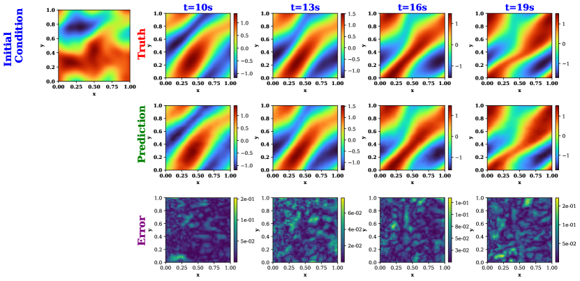
Among all the sampled states, the best-performing state is found to be {$db$4, GeLU, $sym$6, GeLU, $rbio$6.8, GeLU, $db$4, GeLU}. While the states with the highest probability are dominated by the Daubechies wavelets and GeLU activation function, the best-performing state is participated by three different wavelet basis functions. These prediction results of the vorticity fields from the proposed FWNO architecture are illustrated in Fig. 6. The mean estimate of the relative $L^{2}$ error norm over the test dataset is provided in Table 2. In Fig. 6, we observe a similar performance as the previous examples. The architecture constructed by the best-performing state maintains a consistent accuracy over all the prediction time steps. The mean error values in Table 2 are also evidence that the proposed framework outperforms the vanilla WNO architecture.

References

- [1] Michael Renardy and Robert C Rogers. An introduction to partial differential equations, volume 13. Springer Science & Business Media, 2006.
- [2] Arnold Sommerfeld. Partial differential equations in physics. Academic press, 1949.
- [3] Thomas JR Hughes. The finite element method: linear static and dynamic finite element analysis. Courier Corporation, 2012.
- [4] Robert Eymard, Thierry Gallouët, and Raphaèle Herbin. Finite volume methods. In Handbook of numerical analysis, volume 7, pages 713–1018. 2000.
- [5] Tianping Chen and Hong Chen. Universal approximation to nonlinear operators by neural networks with arbitrary activation functions and its application to dynamical systems. IEEE Transactions on Neural Networks, 6(4):911–917, 1995.
- [6] Lu Lu, Pengzhan Jin, and George Em Karniadakis. Deeponet: Learning nonlinear operators for identifying differential equations based on the universal approximation theorem of operators. arXiv preprint arXiv:1910.03193, 2019.
- [7] Sifan Wang, Hanwen Wang, and Paris Perdikaris. Learning the solution operator of parametric partial differential equations with physics-informed deeponets. Science advances, 7(40):eabi8605, 2021.
- [8] Zongyi Li, Nikola Kovachki, Kamyar Azizzadenesheli, Burigede Liu, Kaushik Bhattacharya, Andrew Stuart, and Anima Anandkumar. Neural operator: Graph kernel network for partial differential equations. 2020.
- [9] Zongyi Li, Nikola Kovachki, Kamyar Azizzadenesheli, Burigede Liu, Kaushik Bhattacharya, Andrew Stuart, and Anima Anandkumar. Fourier neural operator for parametric partial differential equations. 2020.
- [10] Tapas Tripura and Souvik Chakraborty. Wavelet neural operator for solving parametric partial differential equations in computational mechanics problems. Computer Methods in Applied Mechanics and Engineering, 404:115783, 2023.
- [11] N Navaneeth, Tapas Tripura, and Souvik Chakraborty. Physics informed wno. Computer Methods in Applied Mechanics and Engineering, 418:116546, 2024.
- [12] Jacob H. Seidman, Georgios Kissas, Paris Perdikaris, and George J. Pappas. Nomad: Nonlinear manifold decoders for operator learning, 2022.
- [13] Qianying Cao, Somdatta Goswami, and George Em Karniadakis. Lno: Laplace neural operator for solving differential equations, 2023.
- [14] V. S. Fanaskov and I. V. Oseledets. Spectral neural operators. Doklady Mathematics, 108(Suppl 2):S226–S232, 2023.
- [15] Martin Wistuba, Ambrish Rawat, and Tejaswini Pedapati. A survey on neural architecture search. arXiv preprint arXiv:1905.01392, 2019.
- [16] Thomas Elsken, Jan Hendrik Metzen, and Frank Hutter. Neural architecture search: A survey. Journal of Machine Learning Research, 20(55):1–21, 2019.
- [17] Pengzhen Ren, Yun Xiao, Xiaojun Chang, Po-yao Huang, Zhihui Li, Xiaojiang Chen, and Xin Wang. A comprehensive survey of neural architecture search: Challenges and solutions. ACM Comput. Surv., 54(4), may 2021.
- [18] Yuqiao Liu, Yanan Sun, Bing Xue, Mengjie Zhang, Gary G Yen, and Kay Chen Tan. A survey on evolutionary neural architecture search. IEEE transactions on neural networks and learning systems, 34(2):550–570, 2021.
- [19] Hieu Pham, Melody Guan, Barret Zoph, Quoc Le, and Jeff Dean. Efficient neural architecture search via parameters sharing. In Jennifer Dy and Andreas Krause, editors, Proceedings of the 35th International Conference on Machine Learning, volume 80 of Proceedings of Machine Learning Research, pages 4095–4104. PMLR, 10–15 Jul 2018.
- [20] Chenxi Liu, Barret Zoph, Maxim Neumann, Jonathon Shlens, Wei Hua, Li-Jia Li, Li Fei-Fei, Alan Yuille, Jonathan Huang, and Kevin Murphy. Progressive neural architecture search. In Proceedings of the European conference on computer vision (ECCV), pages 19–34, 2018.
- [21] Z. Zhong, J. Yan, W. Wu, J. Shao, and C. Liu. Practical block-wise neural network architecture generation. In 2018 IEEE/CVF Conference on Computer Vision and Pattern Recognition (CVPR), pages 2423–2432, Los Alamitos, CA, USA, jun 2018. IEEE Computer Society.
- [22] Bowen Baker, Otkrist Gupta, Nikhil Naik, and Ramesh Raskar. Designing neural network architectures using reinforcement learning, 2017.
- [23] Barret Zoph and Quoc Le. Neural architecture search with reinforcement learning. In International Conference on Learning Representations, 2017.
- [24] Emmanuel Bengio, Moksh Jain, Maksym Korablyov, Doina Precup, and Yoshua Bengio. Flow network based generative models for non-iterative diverse candidate generation. In M. Ranzato, A. Beygelzimer, Y. Dauphin, P.S. Liang, and J. Wortman Vaughan, editors, Advances in Neural Information Processing Systems, volume 34, pages 27381–27394. Curran Associates, Inc., 2021.
- [25] Yoshua Bengio, Salem Lahlou, Tristan Deleu, Edward J. Hu, Mo Tiwari, and Emmanuel Bengio. Gflownet foundations. J. Mach. Learn. Res., 24(1), mar 2024.
- [26] Moksh Jain, Emmanuel Bengio, Alex Hernandez-Garcia, Jarrid Rector-Brooks, Bonaventure F. P. Dossou, Chanakya Ajit Ekbote, Jie Fu, Tianyu Zhang, Michael Kilgour, Dinghuai Zhang, Lena Simine, Payel Das, and Yoshua Bengio. Biological sequence design with GFlowNets. In Kamalika Chaudhuri, Stefanie Jegelka, Le Song, Csaba Szepesvari, Gang Niu, and Sivan Sabato, editors, Proceedings of the 39th International Conference on Machine Learning, volume 162 of Proceedings of Machine Learning Research, pages 9786–9801. PMLR, 17–23 Jul 2022.
- [27] Moksh Jain, Sharath Chandra Raparthy, Alex Hernández-García, Jarrid Rector-Brooks, Yoshua Bengio, Santiago Miret, and Emmanuel Bengio. Multi-objective GFlowNets. In Andreas Krause, Emma Brunskill, Kyunghyun Cho, Barbara Engelhardt, Sivan Sabato, and Jonathan Scarlett, editors, Proceedings of the 40th International Conference on Machine Learning, volume 202 of Proceedings of Machine Learning Research, pages 14631–14653. PMLR, 23–29 Jul 2023.
- [28] Navaneeth N. and Souvik Chakraborty. Waveformer for modeling dynamical systems. Mechanical Systems and Signal Processing, 211:111253, 2024.
- [29] Tapas Tripura, Abhilash Awasthi, Sitikantha Roy, and Souvik Chakraborty. A wavelet neural operator based elastography for localization and quantification of tumors. Computer Methods and Programs in Biomedicine, 232:107436, 2023.
- [30] Akshay Thakur, Tapas Tripura, and Souvik Chakraborty. Multi-fidelity wavelet neural operator with application to uncertainty quantification. arXiv preprint arXiv:2208.05606, 2022.
- [31] Tapas Tripura and Souvik Chakraborty. A foundational neural operator that continuously learns without forgetting. arXiv preprint arXiv:2310.18885, 2023.
- [32] Jyoti Rani, Tapas Tripura, Hariprasad Kodamana, and Souvik Chakraborty. Generative adversarial wavelet neural operator: Application to fault detection and isolation of multivariate time series data. arXiv preprint arXiv:2401.04004, 2024.
- [33] Souvik Chakraborty et al. Dpa-wno: A gray box model for a class of stochastic mechanics problem. arXiv preprint arXiv:2309.15128, 2023.
- [34] Lu Lu, Xuhui Meng, Shengze Cai, Zhiping Mao, Somdatta Goswami, Zhongqiang Zhang, and George Em Karniadakis. A comprehensive and fair comparison of two neural operators (with practical extensions) based on fair data. Computer Methods in Applied Mechanics and Engineering, 393:114778, 2022.