Generative Ensemble Regression: Learning Particle Dynamics from Observations of Ensembles with Physics-Informed Deep Generative Models
Abstract
We propose a new method for inferring the governing stochastic ordinary differential equations (SODEs) by observing particle ensembles at discrete and sparse time instants, i.e., multiple “snapshots”. Particle coordinates at a single time instant, possibly noisy or truncated, are recorded in each snapshot but are unpaired across the snapshots. By training a physics-informed generative model that generates “fake” sample paths, we aim to fit the observed particle ensemble distributions with a curve in the probability measure space, which is induced from the inferred particle dynamics. We employ different metrics to quantify the differences between distributions, e.g., the sliced Wasserstein distances and the adversarial losses in generative adversarial networks (GANs). We refer to this method as generative “ensemble-regression” (GER), in analogy to the classic “point-regression”, where we infer the dynamics by performing regression in the Euclidean space. We illustrate the GER by learning the drift and diffusion terms of particle ensembles governed by SODEs with Brownian motions and Lévy processes up to 100 dimensions. We also discuss how to treat cases with noisy or truncated observations. Apart from systems consisting of independent particles, we also tackle nonlocal interacting particle systems with unknown interaction potential parameters by constructing a physics-informed loss function. Finally, we investigate scenarios of paired observations and discuss how to reduce the dimensionality in such cases by proving a convergence theorem that provides theoretical support.
Introduction
Classic methods for inferring the ordinary differential equation (ODE) dynamics from data usually require observations of a point or particle governed by the ODE at different time instants. We refer this learning paradigm as “point-regression”. More specifically, as illustrated in Figure 1, in point-regression problems we aim to infer the governing ODE of a point and perhaps also the initial condition, given the (possibly noisy) observations of its coordinates at different time instants. Typically, we optimize the dynamics and the initial coordinate so that the inferred curve matches the data in the Euclidean distance. Let us consider, for simplicity, the one-dimensional linear regression with quadratic loss as an example. Given observations of at multiple , we want to optimize the parameter in the ODE as well as the initial point so that the mean squared distance between predictions and data points is minimized, where and are the slope and the intercept of the linear function. Other examples in this category include logistic regression, recurrent neural networks [1] and the neural ODE [2] for time series, etc.
For systems consisting of an ensemble of particles, point-regression may fail to apply. For example, we want to infer the governing stochastic ordinary differential equations (SODE) from observations of particle ensembles at discrete and sparse time instants, but the data of an individual particle are not sufficiently informative for dynamic inference. Another example is a system consisting of a large number of interacting particles, even close to the mean field limit, e.g., we may want to infer how the fish interact with each other from discrete snapshots of the fish school. In such scenarios, instead of learning from individual particles, we need to learn from the particle ensembles. Specifically, we wish to infer the governing dynamics and perhaps also the initial condition, using observations of an ensemble of particle at discrete time instants. We call an observation at a single time instant a “snapshot”, where part or all of the particle coordinates in the ensemble are recorded. Since the particles could be indistinguishable in observations, especially in a large system, we thus consider the case where the data are not labeled with particle indices, in other words, we cannot pair data across snapshots.
We call this paradigm “ensemble-regression” in analogy to the “point-regression”. As illustrated in Figure 1, the initial condition and dynamics for particles would induce a curve in the probability measure space, where denotes the particle distributions at time . Such will be governed by a corresponding partial differential equation (PDE), e.g., the Fokker-Planck equation if the particles are governed by SODEs of diffusion processes. We aim to optimize the dynamics and the initial distribution so that the inferred curve matches the distributions from the data, and the differences can be quantified with certain metrics.


Herein we propose a new method to perform ensemble-regression. We use a generative model with deep neural networks as build blocks, which will generate “fake” particle systems, to represent the inferred curve in the probability measure space, and then perform regression in the probability measure space with the inferred curve. We thus name our method as generative ensemble-regression. In this paper we test the sliced Wasserstein (SW) distance [3] and the loss in generative adversarial networks (GANs) [4, 5] as two examples of metrics, the latter proved to be very effective when analyzing high dimensional data [6] in our problems.
The deep generative model is physics-informed in that our partial physical knowledge of the dynamics will be encoded into the architecture or the loss function. Such physical knowledge is sometimes essential for a correct dynamic inference, since the particle dynamic can be not unique even if the curve and its governing PDE are fully given. For example, the following two particle dynamics with as the initial distribution will lead to the same curve :
-
•
Standard Brownian motion with no drift.
-
•
with no diffusion, i.e., .
However, if we know that the particle dynamic is in the form of , so that is governed by the continuity equation , and is limited to the closure of , then the solution of is unique, for any curve absolutely continuous from to , where is the Wasserstein-2 space of probability measures with finite quadratic moments in [7, 8].
In the generative model, we use discretized ODE or SODE with unknown terms parameterized as neural networks. This is referred as the “neural ODE” and “neural SDE” in the literature [2, 9, 10, 11, 12, 13], but in applications the observations are mainly a time series, i.e., observations of a single particle. The idea of employing a neural networks as velocity surrogates with physics-informed loss functions in particle systems was also used for solving mean field game/control problems [14]. There are other works using GANs to solve inverse problems, including [15], where GANs were applied to learn parameters in time-independent stochastic differential equations, and [16] where GANs were applied to learn the random parameters from the (paired) observations of independent ODEs.
In this paper, we tackle two typical types of particle systems: (1) independent particle systems governed by SODEs, and (2) interacting particle systems governed by nonlocal flocking dynamics. For inferring dynamics governed by SODE, most algorithms are based on observations of a sample path, and perform the inference by calculating or approximating the probability of observations conditioned on the system parameters, using Euler-Maruyama discretization [17, 18], Kalman filtering [19], variational Gaussian process-based approximation [20, 21], etc. There are other works inferring the stochastic dynamics with the (estimated) densities from the perspective of Fokker-Planck equations [22], but this approach is hard to scale to high dimensional problems. For flocking dynamic systems, other researchers infer the key parameters in the influence function by fitting the velocity field via Bayesian optimization [23], or fitting the density field by solving a system of transformed PDEs and optimizing the parameters [24]. But these methods require the knowledge of the initial condition, including the distribution and velocity field.
Problem Setup

We start from a system consisting of an ensemble of particles, where the dynamics of the particles is independent of other particles. The most commonly used stochastic processes in physics and biology are diffusion processes and Lévy processes; in particular, the particle dynamics is governed by the stochastic differential equation:
| (1) |
for diffusion processes, and
| (2) |
for Lévy processes, where is the position of a particle at time with randomly drawn from the initial distribution , is the deterministic drift, and are the -dimensional standard Brownian motion and the -stable symmetric Lévy process, respectively, and is the diffusion coefficient. In the mean field limit, the density of the particles would be governed by Fokker-Planck equations or fractional Fokker-Planck equations. For simplicity, in this work we assume that is a function of while is constant, but, in principle, our proposed method can also tackle the time-dependent case.
Apart from systems consisting of independent particles, we further consider systems where particles interact with each other and the particle distributions exhibit more complicated behavior. As an example, we consider the Cucker-Smale particle model [25], which describes individuals in flocks with nonlocal interactions. The individual or particle motion is characterized by the following governing equations:
| (3) | ||||
where the superscripts denote the index of the particles, is the number of particles in the system, and is the influence function. Here, we set
| (4) |
where is the gamma function, is the dimension of , and is the factor that characterizes the decay rate of particle interactions as the distance grows. In the mean field limit, as grows the density of the particles is governed by the following fractional PDE:
| (5) | ||||
where is the density, is the velocity field, and p.v. means the principle value. Note that determines the fractional order.
We consider the scenario where the data available are the observations of the particles coordinates at different time instants with , namely “snapshots”. In other words, the data for time will be a set of samples drawn from , the particle distributions at . If are observations of the same set of particles and we can distinguish these particles, we refer to these cases as the “paired” observations since we can pair the particles from different snapshots. In other cases, are observations of different sets of particles, or we cannot distinguish the particles. We refer to these cases as the “unpaired” observations. In this paper we mainly focus on the unpaired cases, but we also present some work on the paired cases in Paired Observations section, where we introduce how to reduce the effective dimensionality and we prove a theorem to support the introduced method. For independent particle systems, we assume that we are unaware of and , or we may only know the parametrized forms of these terms, and we aim to infer these terms directly or through a proper parametization. For interacting particle systems, we assume we know the forms of the dynamics and the influence function, i.e., Equation 3 and 4, but need to infer the velocity field and the key parameter .
Physics-informed Generative Model
To perform ensemble regression, we will use a generative model with deep neural networks to represent a curve in the probability measure space. Note that the curve is determined by the initial condition and the governing equation, hence, the generative model consists of two parts. In the first part, we employ a feed-forward neural network to represent . In particular, takes samples from random noise , e.g., Gaussian noise, as input and the generated distribution is intended to approximate , where # denotes the push forward operator. The second part of the generative model will generate “fake” particle trajectories with initial coordinates generated by , and the marginal distribution at time will be used to represent in the curve.
Our knowledge of the physics will be incorporated into the generative model in two ways. For non-interacting particle systems, our knowledge including the form of the drift and diffusion as well as the type of stochastic processes will be directly embedded into the architecture of the generative model in the second part. For interacting particle systems, while we have no direct knowledge of the velocity field, we will enforce the inferred velocity to be consistent with our knowledge of the dynamics with a physics-based soft penalty. In the following, we introduce the details of the learning algorithm for both types of systems separately. A schematic overview of the method is shown in Figure 2.
Non-interacting Particle Systems
For non-interacting particle systems, generating particle trajectories is relatively straightforward by directly applying the discretization of governing SODE or ODE. For example, if the particle trajectories are diffusion processes or Lévy processes, we can use the following forward Euler scheme:
| (6) | ||||
where is the time step, and are i.i.d. standard Gaussian random variables and -stable random variables, respectively. We could represent and with neural networks if they are unknown, or represent the unknown parameters with trainable variables if we know their parameterized form.
Our target is to tune the trainable variables in the generative model, including the parameters in and those for parameterizing and , so that the generated marginal distribution fits the data for each . We thus need to define a distance function to measure the difference between the two input distributions, which can be estimated from samples drawn from the two distributions. Consequently the loss function in non-interacting particle systems is defined as:
| (7) |
where is the empirical distribution induced from the sample set . We will refer to it as the distribution loss.
There could be many ways to define , including Wasserstein distances, maximum mean discrepancy, etc. In this paper we use two approaches to define .
First we choose the squared sliced Wasserstein-2 (SW) distance [26, 3] as the function :
| (8) |
where is the Wasserstein-2 distance, and is the one dimensional distribution induced by projecting onto the direction , defined by
| (9) |
similarly for . is the uniform Hausdorff measure on the sphere . In short, the squared sliced Wasserstein-2 distance is the expectation of the squared Wasserstein-2 distance between the two input measures projected onto uniformly random directions. The sliced Wasserstein-2 distance is exactly the Wasserstein-2 distance for one-dimensional distributions, but is easier to calculate for higher dimensional distributions. We present the details of the estimation in the Supplementary Information section S1.
We also use GANs to obtain . The generative model we introduced above can generate “fake” samples at , and for each , we use a discriminator to discriminate generated samples and real samples from . The adversarial loss given by can act as a metric of the difference between and . In particular, we use WGAN-GP [5] as our version of GANs in our paper, with
| (10) |
and the loss function for each discriminator is defined as
| (11) | ||||
where is the distribution generated by uniform sampling on straight lines between pairs of points sampled from and , and is the gradient penalty coefficient. Here, can be mathematically interpreted as the Wasserstein-1 distance between the two input distributions. WGAN-GP is computationally more expensive than the sliced Wasserstein distance since we need to train the generative model and the discriminators iteratively, but it is more scalable to high dimensional problems, for which we made a comparison in the supplementary information section S1.


Interacting Particle Systems
The straightforward discretization of the governing Equations 3 cannot be directly applied to generate “fake” particle trajectories in interacting particle systems, especially for those with strong nonlocal interactions, since the computational cost for one time step would be , where is the number of particles required so that the system is close to the mean field limit, which makes the learning almost intractable. Instead, we propose to first employ a neural network as a surrogate model of the velocity field in the spatial-temporal domain to generate trajectories, and then apply an additional penalty in the loss function to enforce the velocity field to be consistent with the Equations 3. In this paper we use the forward Euler scheme to generate trajectories:
| (12) | ||||
where is the time step. By employing the surrogate model for velocity, the computational cost for generating the particle trajectories is linear, instead of quadratic, with the number of particles.
To enforce to be consistent with our knowledge of the dynamics of Equations 3, we first randomly generate particle trajectories with Equation 12, denoted as , and then calculate the “forces” applied on these particles by another randomly generated particles , using the formula of interactions in Equations 3, where we replace the unknown parameter with a trainable variable. Meanwhile, from the velocity field we can directly calculate the accelerations for these particles using a material derivative. The forces and accelerations should be consistent with each other. We can thus define an loss:
| (13) | ||||
and we name it as the Newton loss. The time span should cover the time for the latest snapshot , and in this paper we simply set as the ceiling of . To reduce computational cost, the average over time steps in can also be approximated by mini-batch, i.e., taking average over random time steps in each training step.
For one time step, the computational cost is for calculating the force terms and for the acceleration terms. Note that should be larger than or equal to , but can be much less than , thus the total computational cost for can be much less than , and this makes the learning tractable.
In the end, the loss for interacting particle systems will be a combination of the Newton loss and the distribution loss:
| (14) |
where the weight is set as 1 in this paper.
Modifications to the Distributions
In order to provide flexibility and adapt the method to different problems, we can also modify the generated distribution and real data before feeding them to the distance function d and calculate the distribution loss. We present some examples here.
In some cases may have heavy tails, e.g., when the particle trajectories correspond to a Lévy process. The heavy tails could spoil the training, since the rare outlier samples could dominate the loss function. We can choose a suitable bounded map to preprocess both the generated samples and the real data so that the heavy tails are removed. If the observations of the particle coordinates are noisy, we can also perturb the generated samples to add artificial noise. By scaling the artificial noise with trainable variables, the size of the noise in observations can also be learned. If we can only make observations of particles in a specific domain, i.e., the observations are truncated, we will also filter the generated samples using a corresponding mask so that the effective domain for the generated samples and observations are the same.
Computational Results
All the neural networks in the main text are feed-forward neural networks with three hidden layers, each of width 128, except the discriminator for high dimensional problems which is a ResNet with 5 hidden layers, each of width 256, and shortcut connections skipping one hidden layer. We use the leaky ReLu [27] activation function with for the discriminator neural networks in WGAN-GP, while using the hyperbolic tangent activation function for other neural networks. The neural network weights are initialized with the uniform Xavier initializer, and the biases are initialized as 0. The variables for parameterizing the diffusion and noise size are initialized as 0 (before been activated by the softplus function). The drift parameters are initialized as in 1D problems, in high dimensional problems, and randomly initialized with standard Gaussian distribution in 2D problems. The batch size for the distribution loss is 1000 for non-interacting particle systems, except in the 2D problem with truncated observations, where we generate 10000 samples to compensate the loss of samples due to filtering. We use the Adam optimizer [28] with for the cases using the sliced Wasserstein distance, while for the cases with WGAN-GP. The time step in the generative model is set as .
1D Problems: Brownian Motion and Lévy Process
In this section, we test our method on the 1D problems using the sliced Wasserstein distance as . We first consider the SODE with Brownian motion and then with the -stable symmetric Lévy process as the stochastic term:
| (15) | ||||
where , with .
Note that we have no knowledge of in learning. Also, we assume we know that the stochastic term has a constant coefficient but we need to infer it; here the ground truth is . To represent the unknown coefficient, we use a trainable variable rectified by a softplus function , which ensures positivity. As for the drift , we consider the following two cases for both SODE problems. In case 1, we know that the drift is a cubic polynomial of . In this case, we use a cubic polynomial to parameterize , and want to infer the four coefficients and . In case 2, we only know that the drift is a function of and hence we use a neural network to parameterize .
For the SODE problem with Brownian motion, we first prepare a pool of sample paths, then independently draw samples at from the pool as our training data. The results for both cases of drift parameterization are illustrated in Figure 3(a). In the figure, all the densities are estimated using Gaussian kernel density estimation with Scott’s rule, and the inferred densities and the reference densities come from samples produced by the generative model or simulation.
Both cases of drift parameterization provide a good inference of the diffusion coefficient, with an error less than after training steps, in all the runs. When using the cubic polynomial parameterization, the inferred drift fits well with the ground truth, with the relative error about in averaged over three runs. The inferred drift using the neural network only fits the ground truth in the region between -1.5 and 1.5. This is reasonable since the particles mainly concentrate in this region, and we can hardly learn the drift outside this region, where the training data are sparse. However, we note that such an inference of drift is sufficiently good for an accurate time extrapolation of the particle distribution at .
One interesting observation is that in case 1 the inferred densities are more accurate than those estimated from the training data. This is because our knowledge of the governing SODE bridges the limited samples in three snapshots, and as we infer the density at, e.g., , we are not only utilizing the data at but also implicitly leveraging the data at and . We can make an analogy in the context of linear regression: multiple noisy data are helpful for inferring the hidden ground truth, since they are bridged by the regressed linear function. We present a more detailed discussion on this topic in the supplementary information in section S2.
For the SODE problem with Lévy process, we prepare sample paths, then independently draw samples within the region at from the pool as our training data. To prevent instability during the training, we apply double precision and clip the generated -stable random variable in Equation 2 between and .
We first test our method without pre-processing the samples as in the problem with Brownian motion. As we can see in the second row of Figure 3(b), the inferences are far away from the ground truth. This is due to the heavy tail of in the Lévy process: some samples far away from , although rare, could dominate the loss function and spoil the training. To deal with this problem, we then apply a bounded map to all the generated and real samples before feeding them to . The results are shown in the first row of Figure 3(b) where we can see the inferences are much improved. In case 2 where the drift is parameterized by neural networks, the inferred drift outside is better than that in the problem with Brownian motion. This is because the samples are more scattered in the Lévy case.
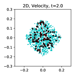
2D Problems: Various Scenarios of Observations
In this section, we test our method on 2D problems using the sliced Wasserstein distance as , with various scenarios of observations. We consider the following 2D SODE:
| (16) |
where
| (17) |
and
| (18) | ||||
The parameters are set as , . We set the initial distribution as . We assume we know that the diffusion coefficient is a constant lower triangular matrix but we need to infer the three unknown parameters . In particular, we use to approximate , where are three trainable variables. Similar as in the 1D problems, we consider the following two cases for the drift. In case 1, we know the form of and in Equation 17 and 18 but we need to infer and ( and are exchangeable). In case 2, we only know that is a gradient of in Equation 17, but we have no knowledge of . In this case, we use a neural network to parameterize .
For the training data, we prepare sample paths, and consider the following various scenarios of observations at . The data are visualized in the supplementary information section S3.
-
•
Scenario 1: we assume that our observations are ideal, i.e., we make accurate observations of all the particle coordinates as the training data.
-
•
Scenario 2: we assume that our observations are noisy. Specifically, we make observations of all the particle coordinates, but each coordinate is perturbed by an i.i.d. random noise , where is set as but also need to be inferred during learning.
-
•
Scenario 3: we assume that our observations are truncated. Specifically, we make observations of the particle coordinates in , with the particles outside of dropped.
For the first scenario, the inferred drift and diffusion are illustrated in Figure 4(a). In case 1, all the inferred drift and diffusion parameters approach the ground truth during the training, with relative error less than for each and less than for each after training steps. In case 2, the inferred diffusion parameters are also close to the ground truth, with error comparable with that in case 1. In the region where the training data are dense (i.e., the density estimated from all the training data is no less than 0.05), the inferred drift field has a relative error about . The inference is much worse in other regions, and the reason is the same as in the 1D problem: the neural network can hardly learn the drift field where the training data are sparse.
For the second and third scenarios, we apply the technique of perturbing and filtering the generated samples, respectively. In Figure 4(b) and Figure 4(c) we show the results of case 1 with the drift parameterized by four parameters. After training steps, all the parameters converge to ground truth. For scenario 2, the error is less than for each drift parameter , less than for each diffusion parameter , and about for the noise parameter . For scenario 3, the error is less than for each drift parameter , less than for each diffusion parameter . We remark that we failed to learn the drift with neural network parameterization in the second and third scenario, suggesting a room for further improvements.


Higher Dimensional Problems
In this section, we test our method on higher dimensional non-interacting particle systems. Note that the sliced Wasserstein distance does not perform well in high dimensional problems, and we thus switch to the WGAN-GP to provide . The comparison between the sliced Wasserstein distance and WGAN-GP in high dimensional problems is presented in the supplementary information section S1.
We consider a -dimensional SODE:
| (19) |
where
| (20) |
for as the -th component of , and is the -th component of . We set the diffusion coefficient matrix as
| (21) |
where the nonzero entries and are set as 1. The initial distribution is . Due to the non-diagonal diffusion coefficient matrix, the motion in different dimensions are coupled.


We prepare sample paths and observe all the particle positions at as our training data. We use a cubic polynomial with four variables to parameterize as a function of for each , while using trainable variables to learn the nonzero entries in the diffusion coefficient matrix, with the diagonal entries rectified by a softplus function for positivity. In other words, we use variables to parameterize the drift and diffusion for the -dimensional SODE. The results are shown in Figure 5. Even for the 100-dimensional problem, after training steps, the average error of the diffusion coefficients is about , and the average relative error of the drift in the interval in each dimension is about .
It may appear surprising that we can solve a 100-dimensional problem with only samples since usually an exponentially large number of samples is required to describe the distribution. However, we remark that the difficulty of the learning task is significantly reduced since our partial knowledge, i.e., the form of the SODE, is encoded into the generator.
Interacting Particle Systems
In this section we consider the 1D and 2D cases of the interacting particle system with governing equations 3. To prepare the training data, we follow [23] and set the initial condition, including the density and velocity as
| (22) | ||||
for the 1D case and
| (23) | ||||
for the 2D case, where is the indicator function. Using the Velocity-Verlet method with time step 0.01, we perform simulations with 1024 and 9976 particles for the 1D and 2D cases, respectively, and generate data at , i.e., 16 snapshots in total. The input radius of the influence function is clipped to be at least , both in simulation and learning, to avoid the singularity. While using the same number of particles and make observations at the same time instants as in [23], our method does not require knowledge of the initial condition or the velocity field in the data snapshots, as opposed to their method based on Bayesian optimization to infer .
We apply the sliced Wasserstein distance for the distribution loss, with the batch size equal to the number of particles in training data. When calculating the distance at each time instant, the generated and real distributions are normalized with the mean and standard deviation of the real distribution. For the Newton loss, we set , and . We use to represent the inferred so that the inference is bounded by 0 and 2, and the variable is initialized as 0.


The results are visualized in Figure 6. For the 1D case, the inferred is 0.492 with ground truth 0.5 in the end of training. As a comparison, the inference is 0.480 for the 1D case in [23]. Our inferred velocity field also matches well with the reference ground truth at different time instants, even at and when we have no observations at all. This is because we incorporated the knowledge of dynamics in the learning system. For the 2D case, while the inferred velocity field also matches well with the ground truth, the inferred is 0.469 with ground truth 0.5 in the end of training, i.e., about 6% error, much larger than in the 1D case. We attribute the error to the fact that the singularity problem for , where the order for is dimension-dependent, is more severe in the 2D case. In supplementary information section S4, we show that as we increase from 0.01 to 0.1, the error is reduced from 6% to 2%. Alternatively, in the 2D case we also try to directly use the data at as the starting coordinates to generate trajectories for ( is also reduced to the data size ), so that the initial generator is removed from the generative model. By doing so, the number of trainable variables is reduced and the learning becomes easier. The inferred is 0.493 in the end of training. As a comparison, the inference is 0.513 for the 2D case in [23]. However, we remark that while this strategy helps to infer without extra data, we cannot infer the velocity or density for .
Paired Observations
We should note that the convergence of the marginal distribution in each snapshot does not necessarily lead to the convergence of the joint distribution of coordinate tuples . While the joint distribution is not available for unpaired observations that we are focused on so far, in other cases where the observed particle coordinates can be paired across snapshots, it is possible to improve the inference by fitting the joint distribution of coordinate tuples with the corresponding generated joint distribution.
In [29], the authors pointed out that Wasserstein convergence of the distribution of is equivalent to Wasserstein convergence of the distributions of for all , if is a Markov chain. However, the sample spaces for are limited to be finite and discrete in [29], thus the result doesn’t apply to dynamic systems in continuous spaces. Here, we present a new theorem for continuous sample spaces:
Theorem 1.
Let be a Markov chain of length and we use to denote the nodes , for . Suppose the domain for is a compact subset of for . We use the () Euclidean metric for all the Euclidean spaces with different dimensions.
Let and be probability measures of for , and be the corresponding probability transition kernels. If converges to in Wasserstein- () metric for all , and as functions of are -Lipschitz continuous in Wasserstein- metric for all and , where is a constant, then converges to in Wasserstein- metric.
We present the proof for Theorem 1 in the supplementary information section S5. The assumption on the continuity of the probability transition kernels is not required for finite discrete sample spaces in [29], but the theorem does not hold without it for continuous sample space. We provide a counter-example in the supplementary information section S6.
The theorem states that under certain conditions, we can set our goal as fitting the distributions of , i.e., coordinate pairs from adjacent snapshots. This should be easier compared with directly fitting the distribution of , since the effective dimensionality is reduced. We still can view this approach as “ensemble-regression”, except that instead of a curve, we try to fit the data with a 2D surface in the probability measure space, where denotes the joint distributions of .


As an illustration, we study the 1D Ornstein–Uhlenbeck (OU) process:
| (24) |
with , so that for any . This is a special example as the governing SODE is not unique given . We make observations of 100 particles at as data, and compare the inferences by fitting the marginal distributions of individual coordinates or the joint distributions of adjacent coordinate pairs using the SW distance. The drift function is parameterized by a linear function or a neural network, while the diffusion coefficient is represented by a trainable variable rectified by a softplus function. We present the results in Figure 7, where we can clearly see the failure in the cases of fitting the marginal distributions, while fitting the joint distributions works very well.
Summary and Discussion
We have proposed a new method for inferring the governing dynamics of particles from unpaired observations of their coordinates at multiple time instants, namely “snapshots”. We fitted the observed particle ensemble distribution with a physics-informed generative model, which can be viewed as performing regression in the probability measure space. We refer to this approach as generative “ensemble-regression”, in analogy to the classic “point-regression”, where we infer the dynamics by performing regression in the Euclidean space.
We first applied the method to particle systems governed by independent stochastic ordinary differential equations (SODE) with Brownian or Lévy noises, where we inferred the drift and the diffusion terms from a small number of snapshots. In the Lévy noise case, we demonstrated that the heavy tails in the distributions could spoil the training, but we addressed this issue by applying a preprocessing map to both the generated and target distributions. In scenarios with noisy or truncated training data, we modified the generated distributions accordingly by perturbing or filtering the generated samples. We then addressed high-dimensional SODE problems using the adversarial loss in GANs. In the end, we managed to learn the parameters for particle interactions in a nonlocal flocking systems.
It is possible to apply our method to learn the interaction parameters for particle-based simulation methods. In particular, we will fit the target mass and velocity distributions coming from the analytical solution or other simulation methods that are accurate but expensive. We leave this promising research direction for future work.
Acknowledgement
This work was supported by the PhILMS grant DE-SC0019453 and by the OSD/AFOSR MURI Grant FA9550-20-1-0358. We would like to thank Prof. Hui Wang and Ms. Tingwei Meng for carefully checking the proof of our theorem. We also want to thank Dr. Zhongqiang Zhang for helpful discussions.
Supplementary Information
S1. Comparison between Sliced Wasserstein Distance and WGAN-GP
The squared sliced Wasserstein-2 distance is the expectation of the squared Wasserstein-2 distance between the two input measures projected onto uniformly random directions. To estimate from samples of and , we use the following process introduced in [3].
-
•
Draw samples independently from and with batch size , denoted as and .
-
•
Uniformly sample projection directions in . In this paper we set .
-
•
For each random direction , project and sort the samples in and in the direction of , getting and , where and for . Calculate .
-
•
Calculate as the estimation of squared .
Compared with GANs, the sliced Wasserstein distance does not need discriminators, and is more robust than WGAN-GP in low dimensional problems. Take the following 1D problem as an example. We consider the SODE:
| (25) |
with . We set so that the exact solution is
| (26) |
We have samples at and , respectively, as the training data, and wish to infer the constant drift and diffusion coefficients. The input noise to the generator is uniform noise from -1 to 1. The results are shown in Figure 8.


We can clearly see oscillations of the inferred drift coefficient for WGAN-GP. This can be attributed to the two-player game between the generator and discriminator, which was also reported in [30].


We did not observe significant oscillations using WGAN-GP in higher dimensional problems. Indeed, WGAN-GP outperforms the sliced Wasserstein distance in high dimensional problems. Let us consider the following simple SODE problem as an example, where the motions are uncoupled between dimensions:
| (27) |
where is the -th component of , with . We prepare sample paths and observe all the particle positions at as our training data. We use a cubic polynomial to parameterize the -th component of the drift. We use another trainable variable rectified by a softplus function to represent the diffusion coefficient in each direction. In total, variables are used to parameterize the -dimensional SODE. The results are shown in Figure 9. While the SW distance works for 2D problems, it does not scale well to high dimensional problems for which WGAN-GP gives much better inferences.
S2. A Study on the Density Estimation
In this section, we wish to show that our method can make use of the SODE and multiple snapshots to reduce the error of density estimation from limited samples. We consider the one-dimensional SODE:
| (28) |
with .
We test the following two cases of training data sets. In both cases we have 1000 samples at , but the particle trajectories are different.
-
•
Case 1: We make observations from different sets of trajectories at different time instants.
-
•
Case 2: We make observations from the same set of trajectories at different time instants.
We assume that we know Equation 28, but have no knowledge of . We could make the analogy of performing linear regression, where we know the slope but do not know the intercept. In Figure 10 we show the comparison between the inferred densities and the densities estimated directly from data. All the densities are estimated using Gaussian kernel density estimation. The inferred densities and the ground truth come from samples produced by the generative model or simulation, with bandwidth decided by the Scott’s rule. To remove the effect of bandwidth selection in the density estimation directly from data, we perform a grid search of the optimal bandwidth factor via the error against ground truth, from 0.01 to 0.5 with grid size 0.01 (Scott’s rule suggests about 0.25).


The grid search strategy is actually infeasible in practice since we don’t know the ground truth, but it should perform better than any bandwidth selector. Despite that, in Figure 10(a) we can clearly see that in case 1 our inferred densities with naive Scott’s rule significantly outperform the ones estimated directly from training data with grid search. This cannot be attributed to the number of samples, since in case 2 the inferred densities with our method cannot perform better, as shown in Figure 10(b).
The different performances in two cases are reasonable. In case 1, our method can utilize the SODE and the observations at multiple time instants to reduce the error from limited samples. As we infer the density at , we are not only utilizing the data at but also implicitly taking advantage of the data at later time instants. In case 2, since the observations come from the same sample paths, the observations at later time instants cannot provide additional information considering that the SODE is already known. Let us again make an analogy in the context of linear regression: if the observations have independent noise, multiple observations will be more helpful than a single observation. However, if the observations have the same noise, multiple observations cannot help us more than a single observation, if we already know the slope.
S3. Training Data in 2D Problems with Various Scenarios of Observations
In Figure 11 we visualize the training data in 2D problems with various scenarios of observations.

S4. Effect of Clipping Radius in the Interacting Particle System

In this section we study the effect of various clipping radius from 0.01 to 0.1, both in the simulation for data generation and the learning algorithm. We remark that changing in this range would not make a huge difference to the system behavior, since the dynamics are dominated by non-local interactions. In Figure 12 we show the inferred during the training. As increase from 0.01 to 0.1, the inferred in the end of training increases from 0.469 to 0.490, with the ground truth 0.5. This suggests that the error mainly comes from the singularity problem of when is small.
S5. Proof for Theorem 1
The proof is based on the weak convergence: convergence of a sequence of probability measures to a probability measure in the Wasserstein- metric is equivalent to the weak convergence plus the convergence of -th moments of to [31]. Here, the weak convergence mean converges to for each , where or , which are equivalent[32]. Note that in Theorem 1 we assume that the domain for is a compact subset of Euclidean space for each , thus is a bounded and continuous function of . The convergence of -th moment then directly comes from the weak convergence, i.e., we only need to show that converges to weakly. This is proved in Lemma 4 below.
The notations are inherited from Theorem 1. For simplicity, we will sometimes use to represent the nodes in sequence, and use to represent the probability measure of , etc.
Lemma 1.
Let mapping from the Euclidean space to the probability measure space be -Lipschitz in Wasserstein- metric (). For any -Lipschitz,
is -Lipschitz.
Proof.
Note that
| (29) | ||||
Firstly
| (30) | ||||
where the first inequality comes from the Kantorovich–Rubinstein formula [31] and that is -Lipschitz. The last inequality comes from that is -Lipschitz in Wasserstein- sense.
Secondly,
| (31) | ||||
We conclude that
| (32) |
i.e. is -Lipschitz ∎
Lemma 2.
If converge to weakly, then converge to weakly.
Proof.
For any bounded and continuous function
| (33) | ||||
The convergence comes from the weak convergence of and that is bounded and continuous as a function of and . ∎
Lemma 3.
Suppose converge to weakly, is Lipschitz in Wasserstein- metric. For any bounded and Lipschitz, we have
| (34) | ||||
Proof.
Since is bounded and continuous, and converge to weakly,
| (35) |
i.e.
| (36) | ||||
Since is bounded and Lipschitz, is Lipschitz, we have
| (37) |
is Lipschitz. Further since converge to weakly (from Lemma 2):
| (38) | ||||
∎
Lemma 4.
Let be a Markov chain of length and we use to denote the nodes , for . Suppose the domain for is a compact subset of for . We use the () Euclidean metric for all the Euclidean spaces with different dimensions.
Let and be probability measures of for , and be the corresponding probability transition kernels. If converges to weakly for all , and are -Lipschitz continuous in Wasserstein- metric for all and , where is a constant, then converges to weakly.
Proof.
We start from the case . For simplicity, we use to denote the nodes in sequence.
For any -Lipschitz and bounded, we have
| (40) | ||||
where
| (41) | ||||
From Lemma 1, since is Lipschitz, is Lipschitz in Wasserstein- sense, we have is Lipschitz. is also bounded since is bounded. So we have
| (42) |
since converge to weakly.
We then need to show converges to 0. We prove by contradiction. Suppose it does not converge, then there exists and a subsequence of (denote as ) such that
| (43) |
Without loss of generality, we assume that
| (44) |
i.e.
| (45) | ||||
Let
| (46) |
then
| (47) | ||||
Note that is -Lipschitz, is -Lipschitz, we have are all -Lipschitz, thus uniformly equicontinuous. Also are uniformly bounded by the bound of , and the domain for is compact (since the domain for is compact for all ). By the Arzela-Ascoli theorem, there exists a subsequence such that uniformly, where is -Lipschitz and bounded. Therefore,
| (48) | ||||
From Lemma 3
| (49) | ||||
We then have
| (50) | ||||
We have a contradiction between Equation 47 and 50. We finish the proof for .
We then prove the case for general by induction. Suppose it holds for , we now prove it for .
From the conditions for the case and that the theorem holds for , we have converges to weakly and converges to weakly. We now view as , view the Cartesian product of as , and view as , so we have converges to weakly and converges to weakly. Also and are -Lipschitz continuious and Wasserstein- metric for all , since and from the Markovian property, and that , . Therefore, from the theorem for case we have that converges to weakly, i.e., converges to weakly.
∎
S6. A Counterexample in Continuous Sample Space
As a direct implementation of Corollary 7 in [29], for the Markov chain in a finite discrete sample space, converges to in Wasserstein- sense for each implies that converges to in Wasserstein- sense. However, if the Markov chains are defined in the continuous sample space, the implementation is, in general, not correct without further assumptions, e.g., the assumption of continuity for probability transition kernels. In this section, we provide a counterexample to show that.
We consider the Markov chain with and use to denote the nodes in sequence. We define as follows:
| (51) | ||||
and as following:
| (52) | ||||
We can easily check that converges to in Wasserstein- metric, since
| (53) | ||||
and
| (54) | ||||
Similarly converges to in Wasserstein- metric. However, does not converge to in Wasserstein- metric: the support of and always have a distance larger than 1.
References
- [1] Sepp Hochreiter and Jürgen Schmidhuber. Long short-term memory. Neural computation, 9(8):1735–1780, 1997.
- [2] Tian Qi Chen, Yulia Rubanova, Jesse Bettencourt, and David K Duvenaud. Neural ordinary differential equations. In Advances in Neural Information Processing Systems, pages 6571–6583, 2018.
- [3] Ishan Deshpande, Ziyu Zhang, and Alexander G Schwing. Generative modeling using the sliced Wasserstein distance. In Proceedings of the IEEE Conference on Computer Vision and Pattern Recognition, pages 3483–3491, 2018.
- [4] Ian Goodfellow, Jean Pouget-Abadie, Mehdi Mirza, Bing Xu, David Warde-Farley, Sherjil Ozair, Aaron Courville, and Yoshua Bengio. Generative adversarial nets. In Advances in Neural Information Processing Systems, pages 2672–2680, 2014.
- [5] Ishaan Gulrajani, Faruk Ahmed, Martin Arjovsky, Vincent Dumoulin, and Aaron C Courville. Improved training of Wasserstein GANs. In Advances in Neural Information Processing Systems, pages 5767–5777, 2017.
- [6] David L Donoho et al. High-dimensional data analysis: The curses and blessings of dimensionality. AMS math challenges lecture, 1(2000):32, 2000.
- [7] Luigi Ambrosio, Nicola Gigli, and Giuseppe Savaré. Gradient flows: in metric spaces and in the space of probability measures. Springer Science & Business Media, 2008.
- [8] Luigi Ambrosio and Wilfrid Gangbo. Hamiltonian ODEs in the Wasserstein space of probability measures. Communications on Pure and Applied Mathematics: A Journal Issued by the Courant Institute of Mathematical Sciences, 61(1):18–53, 2008.
- [9] Xuechen Li, Ting-Kam Leonard Wong, Ricky TQ Chen, and David Duvenaud. Scalable gradients for stochastic differential equations. arXiv preprint arXiv:2001.01328, 2020.
- [10] Junteng Jia and Austin R Benson. Neural jump stochastic differential equations. In Advances in Neural Information Processing Systems, pages 9843–9854, 2019.
- [11] Xuanqing Liu, Tesi Xiao, Si Si, Qin Cao, Sanjiv Kumar, and Cho-Jui Hsieh. Neural SDE: Stabilizing neural ODE networks with stochastic noise. arXiv preprint arXiv:1906.02355, 2019.
- [12] Belinda Tzen and Maxim Raginsky. Neural stochastic differential equations: Deep latent Gaussian models in the diffusion limit. arXiv preprint arXiv:1905.09883, 2019.
- [13] Belinda Tzen and Maxim Raginsky. Theoretical guarantees for sampling and inference in generative models with latent diffusions. arXiv preprint arXiv:1903.01608, 2019.
- [14] Lars Ruthotto, Stanley J Osher, Wuchen Li, Levon Nurbekyan, and Samy Wu Fung. A machine learning framework for solving high-dimensional mean field game and mean field control problems. Proceedings of the National Academy of Sciences, 117(17):9183–9193, 2020.
- [15] Liu Yang, Dongkun Zhang, and George Em Karniadakis. Physics-informed generative adversarial networks for stochastic differential equations. SIAM Journal on Scientific Computing, 42(1):A292–A317, 2020.
- [16] Junyu Liu, Zichao Long, Ranran Wang, Jie Sun, and Bin Dong. RODE-Net: Learning ordinary differential equations with randomness from data. arXiv preprint arXiv:2006.02377, 2020.
- [17] Ola Elerian, Siddhartha Chib, and Neil Shephard. Likelihood inference for discretely observed nonlinear diffusions. Econometrica, 69(4):959–993, 2001.
- [18] Bjørn Eraker. MCMC analysis of diffusion models with application to finance. Journal of Business & Economic Statistics, 19(2):177–191, 2001.
- [19] Simo Särkkä, Jouni Hartikainen, Isambi Sailon Mbalawata, and Heikki Haario. Posterior inference on parameters of stochastic differential equations via non-linear Gaussian filtering and adaptive MCMC. Statistics and Computing, 25(2):427–437, 2015.
- [20] Cedric Archambeau, Dan Cornford, Manfred Opper, and John Shawe-Taylor. Gaussian process approximations of stochastic differential equations. Journal of Machine Learning Research, 1:1–16, 2007.
- [21] Michail D Vrettas, Manfred Opper, and Dan Cornford. Variational mean-field algorithm for efficient inference in large systems of stochastic differential equations. Physical Review E, 91(1):012148, 2015.
- [22] Joseph Bakarji and Daniel M Tartakovsky. Data-driven discovery of coarse-grained equations. Journal of Computational Physics, page 110219, 2021.
- [23] Zhiping Mao, Zhen Li, and George Em Karniadakis. Nonlocal flocking dynamics: Learning the fractional order of pdes from particle simulations. Communications on Applied Mathematics and Computation, 1(4):597–619, 2019.
- [24] Christos N Mavridis, Amoolya Tirumalai, and John S Baras. Learning interaction dynamics from particle trajectories and density evolution. In 2020 59th IEEE Conference on Decision and Control (CDC), pages 1014–1019. IEEE, 2020.
- [25] Felipe Cucker and Steve Smale. Emergent behavior in flocks. IEEE Transactions on automatic control, 52(5):852–862, 2007.
- [26] Filippo Santambrogio. Euclidean, metric, and Wasserstein gradient flows: an overview. Bulletin of Mathematical Sciences, 7(1):87–154, 2017.
- [27] Andrew L Maas, Awni Y Hannun, and Andrew Y Ng. Rectifier nonlinearities improve neural network acoustic models. In Proceedings of the International Conference on Machine Learning, volume 30, page 3, 2013.
- [28] Diederik P Kingma and Jimmy Ba. Adam: A method for stochastic optimization. arXiv preprint arXiv:1412.6980, 2014.
- [29] Mucong Ding, Constantinos Daskalakis, and Soheil Feizi. Subadditivity of probability divergences on Bayes-Nets with applications to time series GANs. CoRR, abs/2003.00652, 2020.
- [30] Constantinos Daskalakis, Andrew Ilyas, Vasilis Syrgkanis, and Haoyang Zeng. Training GANs with optimism. In International Conference on Learning Representations, 2018.
- [31] Cédric Villani. Optimal transport: old and new, volume 338. Springer Science & Business Media, 2008.
- [32] Achim Klenke. Probability theory: a comprehensive course. Springer Science & Business Media, 2013.