Generating Smooth Pose Sequences for Diverse Human Motion Prediction
Abstract
Recent progress in stochastic motion prediction, i.e., predicting multiple possible future human motions given a single past pose sequence, has led to producing truly diverse future motions and even providing control over the motion of some body parts. However, to achieve this, the state-of-the-art method requires learning several mappings for diversity and a dedicated model for controllable motion prediction. In this paper, we introduce a unified deep generative network for both diverse and controllable motion prediction. To this end, we leverage the intuition that realistic human motions consist of smooth sequences of valid poses, and that, given limited data, learning a pose prior is much more tractable than a motion one. We therefore design a generator that predicts the motion of different body parts sequentially, and introduce a normalizing flow based pose prior, together with a joint angle loss, to achieve motion realism. Our experiments on two standard benchmark datasets, Human3.6M and HumanEva-I, demonstrate that our approach outperforms the state-of-the-art baselines in terms of both sample diversity and accuracy. The code is available at https://github.com/wei-mao-2019/gsps
![[Uncaptioned image]](https://cdn.awesomepapers.org/papers/f3146a74-1427-4426-a099-57b30bad6df2/x1.png) |
1 Introduction
Predicting future human motions from historical pose sequences has broad applications in autonomous driving [42], animation creation in the game industry [52] and human robot interaction [33]. Most existing work focuses on deterministic prediction, namely, predicting only the most likely future sequence [16, 41, 35, 39, 38]. However, future human motion is naturally diverse, especially over a long-term horizon (s).
Most of the few attempts to produce diverse future motion predictions exploit variational autoencoders (VAEs) to model the multi-modal data distribution [53, 56, 4]. These VAEs-based models are trained to maximize the motion likelihood. As a consequence, and as discussed in [57], because training data cannot cover all possible diverse motions, test-time sampling tends to concentrate on the major data distribution modes, ignoring the minor ones, and thus limiting the diversity of the output. To address this Yuan et al. [57] proposed to learn multiple mapping functions, which produce multiple predictions that are explicitly encouraged to be diverse. While this framework indeed yields high diversity, it requires training several mappings in parallel, and separates the training of such mappings from that of the VAE it employs for prediction. Furthermore, while the approach was shown to be applicable to controllable motion prediction, doing so requires training a dedicated model and does not guarantee the controlled part of the motion, e.g., the lower body, to be truly fixed to the same motion in different predictions as the remaining body parts vary.
 |
 |
| (a) | (b) |
In this paper, we introduce an end-to-end trainable approach for diverse motion prediction that does not require learning several mappings to achieve diversity. Our framework yields fully controllable motion prediction; one can strictly fix the motion of one portion of the human body and generate diverse predictions for the other portion only.
To this end, we rely on the observation that diverse future motions are composed of valid human poses organized in smooth sequences. Therefore, instead of learning a motion prior/distribution, for which sufficiently diverse training data is hard to obtain, we propose to learn a pose prior and enforce a hard constraint on the predicted poses to form smooth sequences and to satisfy human kinematic constraints. Specifically, we model our pose prior as a normalizing flow [47, 15], which allows us to compute the data log-likelihood exactly, and further promote diversity by maximizing the distance between pairs of samples during training.
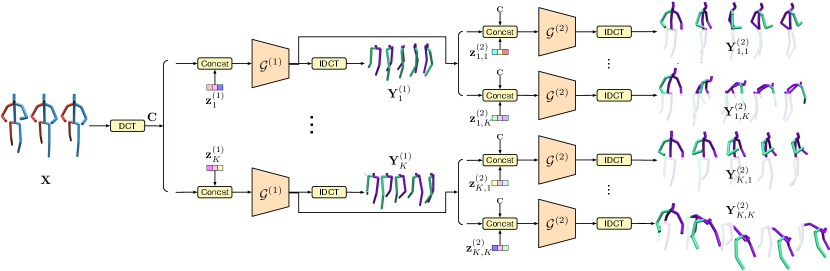
To achieve controllable motion predictions, as illustrated in Fig. 2 (a), we generate the future motions of the different body parts of interest in a sequential manner. Our design allows us to produce diverse future motions that share the same partial body motion, e.g., the same leg motion but diverse upper-body motions. This is achieved by fixing the latent codes for some body parts while varying those of the other body parts. In contrast to [57], our approach allows us to train a single model that achieves both non-controllable and controllable motion prediction.
Our contributions can be summarized as follows: (i) We develop a unified framework achieving both diverse and part-based controllable human motion prediction, using a pre-ordered part sequence; (ii) We propose a pose prior and a joint angle constraint to regularize the training of our generator and encourage it to produce smooth pose sequences. Such strategy overcomes the difficulty of learning the distribution of diverse motions as other VAE-based methods do.
Our experiments on standard human motion prediction benchmarks demonstrate that our approach outperforms the state-of-the-art methods in terms of sample diversity and accuracy.
2 Related Work
Human motion prediction. Early attempts at human motion prediction [9, 48, 51, 55] relied on non-deep learning approaches, such as Hidden Markov Model [9] and Gaussian Process latent variable models [55]. Despite their success on modeling simple periodic motions, more complicated ones are typically better handled via deep neural networks. Deep learning based methods can be roughly categorized into deterministic approaches and stochastic ones.
Deterministic models focus on predicting the most likely human future motion sequence given historical observations [16, 27, 10, 41, 46, 19, 35, 3, 39, 54, 18, 38, 11, 40]. Motivated by the success of RNNs for sequence modeling [50, 32], many such methods employ recurrent architectures [16, 27, 41, 46, 19, 18]. Nevertheless, feed-forward models have more recently been shown to effectively leverage the human kinematic structure and long motion history [35, 39, 3, 10]. In any event, while deterministic human motion prediction models have achieved promising results, especially for short-term prediction (s), they struggle with predictions for long-term horizons (s). This is because human motion is an inherently stochastic process, where one observed motion can lead to multiple possible future ones.
Addressing this has been the focus of stochastic motion prediction methods. Existing ones are mainly based on deep generative models [53, 36, 6, 22, 34, 56, 4, 57], such as variational autoencoders (VAEs) [30] and generative adversarial networks (GANs) [17]. In the context of VAE-based ones, Yan et al. [56] proposed to jointly learn a feature embedding for motion reconstruction and a feature transformation to model the motion mode transitions; Aliakbarian et al. [4] introduced a perturbation strategy for the random variable to prevent the generator from ignoring it. In both cases, once the generator is trained, possible future motions are obtained by feeding it randomly-sampled latent codes. However, as argued in [57], such likelihood-based sampling strategy concentrates on the major mode(s) of the data distribution while ignoring the minor ones. To address this, Yuan et al. [57] introduced a learnable sampling strategy equipped with a prior explicitly encouraging the diversity of the future predictions obtained from a pre-trained generator. Despite their promising performance, their future predictions are constrained by the use of a pre-trained generator. As an alternative to VAE-based models, GAN-based methods [36, 6, 22, 34] train the generator jointly with a discriminator. While, in principle, one could also employ a diversity-promoting prior in these methods, in practice, the resulting additional constraints further complicate the inherently-difficult training process [5]. As such, existing GAN-based methods tend to produce limited diversity. Here, instead of using a discriminator to regularize the generation process, we employ a normalizing-flow-based pose prior, accounting for the fact that training data can more easily cover the diversity of poses than that of motions, and encourage the resulting poses to be valid and form smooth sequences.
3D human pose prior. In the 3D human pose estimation literature, many works [8, 45, 59] have attempted to learn 3D pose priors to avoid invalid human poses. Such priors include Gaussian mixture models [8] and VAEs [45]. However, as discussed in [59], these priors only approximate the pose log-likelihood and may lead to instability [59]. To evaluate the exact log-likelihood, Zanfir et al. [59] thus proposed a normalizing flow based pose prior. Normalizing flows (NFs) [47, 15] have recently become popular for density estimation precisely because they allow one to compute the exact log-likelihood. Here, we use a pre-trained NF model to evaluate the log-likelihood of the generated future poses, and by maximizing the log-likelihood, encourage the generator to produce realistic poses.
Joint angle constraint. Joint angle limits have been explored for the task of human pose estimation [21, 12, 1, 13]. In particular, Akhter et al. [1] introduced a pose-dependent joint limit function learned from a motion capture dataset. However, their function is non-differentiable, which makes it ill-suited for deep neural networks. Our angle loss is similar to that of [13]. However, unlike Dabral et al. [13] who only consider angle constraints on arms and legs, consisting of manually-defined valid angle ranges, we encompass all angles between different body parts/joints and exploit the training data to determine the valid angle ranges.
Controllable motion prediction. To the best of our knowledge, Dlow [57] constitutes the only attempt at controllable motion prediction, e.g, fixed lower-body motion but diverse upper-body motions. This was achieved by training a dedicated model, different from the uncontrollable one, yet sill not guaranteeing absolute control of the body parts that should undergo the same motion. By contrast, we develop a unified model that can achieve both controllable and uncontrolled diverse motion prediction, while guaranteeing the controlled parts to truly follow a fixed motion.
Controllable motion prediction/generation has also been studied in computer graphics, specifically for virtual character control [24, 23, 37]. These works focus on generating human motions for a specific goal, such as following a given path or performing pre-defined actions. In particular, [37] relies on a motion VAE to capture motion dynamics and searches for motions that achieve the desired task via sampling policies, while accounting for neither motion diversity nor the detailed body movements. By contrast, our work aims to predict diverse future motions and control the detailed motion of body parts.
3 Our Approach
Let us now introduce our approach to diverse and controllable motion prediction. We represent a human pose as the concatenation of 3D joint coordinates in a single frame. Given a past motion sequence of frames, we aim to predict a set of poses representing a possible future motion. To this end, we rely on a deep generative model, which we design to yield diversity and allow for controllable motion prediction, as discussed below.
 |
 |
| (a) | (b) |
3.1 Diverse Motion Prediction
In this section, we first briefly review the use of deep generative models in the context of human motion prediction and then introduce our solution for diverse prediction.
Deep Generative Models. Let denote the data distribution of future motions , where is the set of all possible future motions, conditioned on past motions , with encompassing all possible motion history. By introducing a latent variable , the data distribution can be reparameterized as , where is a Gaussian distribution. Generating a future motion can then be achieved by sampling a latent variable and mapping it to using a deterministic generator function . Formally, this is expressed as
| (1) | ||||
| (2) |
where the generator is commonly implemented as a deep neural network. To train such a generator, VAE-based methods [56, 4] typically rely on maximizing the evidence lower bound (ELBO) of the motion likelihood, i.e., minimizing the data reconstruction error and the KL divergence. However, this does not encourage diversity across different randomly-sampled vectors ; instead it focuses on maximizing the likelihood of the training motions, and test-time diversity is thus limited by that of the training motions.
To overcome this, we propose to explicitly generate future motions for each sample during training, and explicitly promote their diversity. Because we aim for diversity, we cannot encourage all generated motions to match the ground truth. Therefore, we redefine the reconstruction error so that at least one of them is close to the ground truth. This yields the loss
| (3) |
where indexes over the generated motions for one sample.
This loss, however, imposes constraints on only one of the generated motions. To better constrain the others, we leverage the intuition that, while the dataset contains only one ground-truth future motion for each past motion, several sequences have similar past motions. For each past motion, we therefore search for the training samples with similar past motions, based on a distance threshold, and take their future motion as pseudo ground truth. Let denote the resulting pseudo ground truths. Then, we define the multi-modal reconstruction error
| (4) |
where . It encourages our generator to cover each pseudo ground truth with at least one sampled motion.
To further explicitly encourage diversity across the generated motions, following [57], we use the diversity-promoting loss
| (5) |
where is a normalizing factor.
One drawback of this diversity loss, however, is that it may lead the model to produce unrealistic and physically-invalid motions, particularly if above, which leaves some motions unregularized. The most straightforward way to overcome this would be to learn a motion prior. This, however, would require an impractically large amount of training data. Instead, we therefore leverage the observation that natural motions are composed of valid human poses and thus introduce the pose prior and angle losses discussed below.
Pose prior. We model our pose prior using a normalizing flow [47, 15], which is an invertible transformation that aims to transfer an unknown data distribution to a distribution with a tractable density function, e.g., a Gaussian distribution. In other words, we model the 3D human pose distribution by learning a bijective and differentiable function, which maps a pose sample to a latent representation following a standard Gaussian distribution, i.e., .
Following the normalizing flow literature [47, 15], this allows us to compute the likelihood of a pose as
| (6) |
where and is the determinant of the Jacobian matrix of .
In practice, the function is modeled via a deep network. Considering model size and inference efficiency, we choose a simple network with only 3 fully-connected layers, which is in stark contrast with the much larger architectures in the recent normalizing flow literature [15, 29, 43, 25]. To ensure that is invertible, we compute the weights of each layer via a QR decomposition and use monotonic activation functions. More details about our normalizing flow architecture are provided in the supplementary material.
Given a dataset of valid human poses, we learn the function by maximizing the log-likelihood of the samples in . This can be written as
| (7) | ||||
| (8) |
Given the trained function , we then define a loss function to encourage our generator to produce valid poses. Specifically, we write it as the negative log-likelihood of a generated human pose , which yields
| (9) | ||||
| (10) |
where and .
Joint angle loss. In addition to our learnt pose prior, we leverage the fact that human movements are constrained by the physiological structure of the human body, e.g., one cannot turn their head fully backwards. In our context, this means that the angles between some body parts are limited to a certain range. Here, instead of manually encoding these different ranges, we discover them by analysing a valid human pose dataset .
To this end, as shown in Fig. 4, we first compute unit length vectors, which represent either the orientations of body parts or the directions of limbs. A body part orientation is the normal of the plane defined by 3 joints. For example, the torso plane, shown in blue in Fig. 4 (a), is defined by the left and right shoulders and the pelvis. A limb direction is defined by 2 joints of the limb. We then compute the angle between those vectors for every pose in and define the valid range based on the minimal and maximal such angle. We list all angles and their valid ranges in the supplementary material.
Let denote the pre-defined angles, and and the lower bound and upper bound of angle , respectively. Given a human pose , we write our joint angle loss for as
| (11) |
where is the angle value calculated from pose . We then combine the different angles in our final angle loss .
Predicting smooth trajectory. In the stochastic motion prediction literature, human movements are commonly represented by a sequence of 3D joint coordinates. With such a representation, encouraging the generated poses to be valid, as discussed above, does not ensure that the resulting sequence will look natural. To enforce temporal smoothness, we therefore adopt a trajectory representation based on the Discrete Cosine Transform (DCT), as suggested in [39]. In particular, using a reduced number of low-frequency DCT components guarantees the resulting trajectory to be smooth as shown in Fig. 5.

Specifically, given the past motion sequence , we first replicate the last pose times to generate a temporal sequence of length , where is the length of the future sequence to predict. We then compute the DCT coefficients of this sequence as
| (12) |
where and each column of represents a predefined DCT basis; and each row of is the trajectory of a joint coordinate; and each row of represents the first DCT coefficients for a trajectory.
We then make our generator predict the DCT coefficients of the future motion given those of the past motion . Given the predicted coefficients, we recover the future motion via inverse DCT as
| (13) |
where and . As in [39], our generator also outputs the past motion to encourage the transition from past poses to future ones to be smooth. See the supplementary material for more detail.
| Method | Human3.6M [26] | HumanEva-I [49] | |||||||||
| APD | ADE | FDE | MMADE | MMFDE | APD | ADE | FDE | MMADE | MMFDE | ||
| ERD [16] | 0 | 0.722 | 0.969 | 0.776 | 0.995 | 0 | 0.382 | 0.461 | 0.521 | 0.595 | |
| acLSTM [60] | 0 | 0.789 | 1.126 | 0.849 | 1.139 | 0 | 0.429 | 0.541 | 0.530 | 0.608 | |
| Pose-Knows [53] | 6.723 | 0.461 | 0.560 | 0.522 | 0.569 | 2.308 | 0.269 | 0.296 | 0.384 | 0.375 | |
| MT-VAE [56] | 0.403 | 0.457 | 0.595 | 0.716 | 0.883 | 0.021 | 0.345 | 0.403 | 0.518 | 0.577 | |
| HP-GAN [6] | 7.214 | 0.858 | 0.867 | 0.847 | 0.858 | 1.139 | 0.772 | 0.749 | 0.776 | 0.769 | |
| BoM [7] | 6.265 | 0.448 | 0.533 | 0.514 | 0.544 | 2.846 | 0.271 | 0.279 | 0.373 | 0.351 | |
| GMVAE [14] | 6.769 | 0.461 | 0.555 | 0.524 | 0.566 | 2.443 | 0.305 | 0.345 | 0.408 | 0.410 | |
| DeLiGAN [20] | 6.509 | 0.483 | 0.534 | 0.520 | 0.545 | 2.177 | 0.306 | 0.322 | 0.385 | 0.371 | |
| DSF [58] | 9.330 | 0.493 | 0.592 | 0.550 | 0.599 | 4.538 | 0.273 | 0.290 | 0.364 | 0.340 | |
| DLow [57] | 11.741 | 0.425 | 0.518 | 0.495 | 0.531 | 4.855 | 0.251 | 0.268 | 0.362 | 0.339 | |
| Ours | 14.757 | 0.389 | 0.496 | 0.476 | 0.525 | 5.825 | 0.233 | 0.244 | 0.343 | 0.331 | |
3.2 Controllable Motion Prediction
The diverse motion prediction framework discussed above does not provide any control over the generated motions. For controllable motion prediction, our goal is to predict future sequences that share the same motion for parts of the body while being diverse for the other parts, e.g., same leg motion but diverse upper-body motion. To this end, instead of directly modeling the joint data distribution as discussed above, we propose to model a product of sequential conditional distributions.
Specifically, let a human motion be split into different body part motions, that is, , where defines the motion of the body part, e.g., the left leg. Then, the future body motion distribution can be expressed as
|
. |
(14) |
Each of the conditional distributions describes the motion of a particular body part given the motion of the previous body parts. Similar to the standard deep generative model discussed above, we model each conditional distribution as
| (15) |
| (16) |
where and is a standard Gaussian distribution . In other words, to compute a future motion, we sample different random variables and decode them sequentially to obtain the future motion of each body part. By fixing some random variables while varying the others , our model can generate multiple times the same motion for body parts while producing diverse motions for the other body parts .
Note that our generator design lets us achieve both diverse and controllable motion prediction at the same time. During training, for each past motion of the -th body part, we generate motions for the -th body part leading to future motions given one past motion. For example, as illustrated in Fig. 3, we sample different leg motions and for each leg motion , we generate different upper-body motions . In this context, we then re-write our diversity-promoting loss as a per-body-part loss, leading to
| (17) |
where is the index of the body part, and is the -th future motion for the -th body part111Note that we eliminate the sample index of previous body parts for simplicity. For example, the -th future motion of the nd body part should be represented as , where is the sample index of the st body part.. Altogether, our final training loss is then expressed as
| (18) |
where is the number of body parts.
In practice, inspired by [39], we define each generator as a Graph Convolutional Network (GCN) [31] with several graph convolution layers. Given a feature map , each such layer computes a transformed feature map as , where represents a fully connected graph with learnable connectivity and is a matrix of trainable weights. The details of our network architecture are provided in the supplementary material.
4 Experiments
4.1 Dataset
Following [57], we evaluate our method on 2 motion capture datasets, Human3.6M [26] and HumanEva-I [49], and adopt the same training and testing settings as in [57] on both datasets.
Human3.6M consists of 7 subjects performing 15 actions. We use 5 subjects (S1, S5, S6, S7, S8) for training and the remaining 2 subjects (S9, S11) for testing. We use the original frame rate (50 Hz) and a 17-joint skeleton. We remove the global translation. Our model is trained to observe 25 past frames (0.5s) and predict 100 future frames (2s).
HumanEva-I consists of 3 subjects performing 5 actions, depicted by videos captured at 60 Hz. A person is represented by a 15-joint skeleton. We adopt the official train/test split [49] and also remove the global translation. The model predicts 60 future frames (1s) given 15 past frames (0.25s).
4.2 Metrics, Baselines & Implementation
Metrics. We follow the same evaluation protocol as in [57] to measure diversity and accuracy. (1) To measure the prediction diversity, we use the Average Pairwise Distance (APD) defined as . (2) To measure the reconstruction accuracy over the whole sequence, we use the Average Displacement Error (ADE) computed as . (3) To measure the reconstruction accuracy of the last future pose, we use the Final Displacement Error (FDE) defined as . We further report (4) the multi-modal version of ADE (MMADE), similar to , and (5) the multi-modal version of FDE (MMFDE).
| APD | Human3.6M [26] | HumanEva-I [49] | |||
| Lower | Upper | Lower | Upper | ||
| BoM [7] w/ Eq. 14 | 0 | 4.408 | 0 | 1.319 | |
| DLow [57]-Control | 1.071 | 12.741 | 0.937 | 4.671 | |
| DLow [57] w/ RS | 0.780 | 7.280 | 0.571 | 1.821 | |
| Ours | 0 | 13.150 | 0 | 5.096 | |
Baselines. We compare our method with 3 types of baselines. (1) Deterministic motion prediction methods, including ERD [16] and acLSTM [60]; (2) Stochastic motion prediction methods without diversity-promoting technique, including CVAE based methods, Pose-Knows [53] and MT-VAE [56], as well as a CGAN based method, HP-GAN [6]; (3) Diverse motion prediction methods, including BoM [7], GMVAE [14], DeLiGAN [20], DSF [58], and DLow [57]. The results of all baselines are directly reported from[57].
| Human3.6M [26] | HumanEva-I [49] | ||||||||||||||||
|---|---|---|---|---|---|---|---|---|---|---|---|---|---|---|---|---|---|
| APD | ADE | FDE | MMADE | MMFDE | NLL | APD | ADE | FDE | MMADE | MMFDE | NLL | ||||||
| ✓ | ✓ | ✓ | ✓ | 15.257 | 0.389 | 0.497 | 0.477 | 0.527 | 251.190 | 7.574 | 0.245 | 0.293 | 0.416 | 0.430 | 363.838 | ||
| ✓ | ✓ | ✓ | ✓ | 19.608 | 0.397 | 0.534 | 0.506 | 0.575 | 97.774 | 6.569 | 0.235 | 0.276 | 0.406 | 0.410 | 119.673 | ||
| ✓ | ✓ | ✓ | ✓ | 6.318 | 0.370 | 0.488 | 0.478 | 0.529 | 64.731 | 2.048 | 0.214 | 0.259 | 0.384 | 0.398 | 75.375 | ||
| ✓ | ✓ | ✓ | ✓ | 20.030 | 0.479 | 0.562 | 0.513 | 0.569 | 89.726 | 6.778 | 0.567 | 0.625 | 0.606 | 0.633 | 109.777 | ||
| ✓ | ✓ | ✓ | ✓ | 18.079 | 0.394 | 0.538 | 0.520 | 0.587 | 91.977 | 6.474 | 0.234 | 0.283 | 0.415 | 0.421 | 113.630 | ||
| ✓ | ✓ | ✓ | ✓ | ✓ | 14.757 | 0.389 | 0.496 | 0.476 | 0.525 | 74.872 | 5.826 | 0.233 | 0.244 | 0.343 | 0.331 | 103.306 | |
Implementation. We set the hidden size of the generator to 256 and the dimension of the random variable to 64. To compare with the controllable version of DLow [57], we divide a human pose into 2 parts: lower and upper body (). We also provide qualitative results for in our supplementary material. The number of samples is set to 10. Thus, during training, we predict 10 future lower body motions, and for each motion, we generate 10 upper body motions. For Human3.6M, the model is trained using a batch size of 16 for 500 epoch with 5000 training examples per epoch. The weights of the different loss terms and the normalizing factors are set to and , respectively. For HumanEva-I, the model is trained using a batch size of 16 for 500 epoch with 2000 training examples per epoch. The weights of different loss terms and the normalizing factors are set to and , respectively. Additional implementation details are provided in the supplementary material.
4.3 Results
Diverse Motion Prediction. In Table 1, we compare our results with the baselines on Human3.6M and HumanEva-I. For all stochastic motion prediction baselines, the results are computed over 50 future motions per test sequence.
Our method consistently outperforms all baselines on all metrics. In general, stochastic motion prediction methods outperform deterministic ones in accuracy (ADE, FDE, MMADE, MMFDE). The reason is that, for multi-modal datasets, deterministic prediction models tend to predict an average mode, which leads to higher errors. For stochastic motion prediction, there is a trade-off between sample diversity (APD) and accuracy. One can achieve high diversity while sacrificing some performance in accuracy, e.g., DSF [58], or vice versa, e.g., BoM [7].
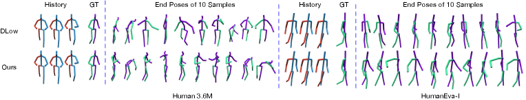
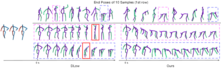
Let us now focus on DLow [57], which constitutes the state of the art. Although, its learnable sampling strategy balances diversity and accuracy well, leading to better results than the other baselines, our method outperforms it on all metrics for both datasets. Note that, on Human3.6M, our method achieves lower reconstruction error (ADE) with higher sample diversity (APD). The qualitative comparisons in Fig. 6 further evidence that our predictions are closer to the GT and more diverse. We further provide a detailed comparison in Fig. 7, which shows that DLow [57] still produces some invalid poses, highlighted with red boxes. This can be caused by its lack of a pose-level prior.
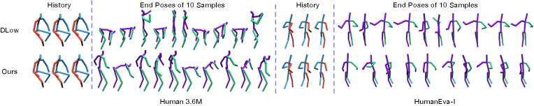
Controllable Motion Prediction. We also compare our method with DLow for controllable motion prediction in Table 2. Here, the prediction model aims to predict future motions with the same lower-body motion but diverse upper-body motions. Our method gives a full control of the lower-body with higher diversity on upper-body. By contrast, DLow [57] cannot guarantee the lower-body motion for different samples to be exactly the same. Although rejection sampling222For each test sequence, we sampled 1000 future motions and chose the 50 with lower-body motion closest to the target one. helps to achieve a better control of the lower-body motion (third row), the diversity of upper body motion also drops. In Fig. 8, we compare our results with those of DLow [57], which further supports our conclusions. Moreover, DLow [57] requires a different model for controllable motion prediction, whereas our method yields a unified model able to achieve diverse and controllable motion prediction jointly. We further adapt our conditional formulation (Eq. 14) to one of the most recent baselines (BoM [7]). The results in Table 2 confirm that it also applies to other generators.
4.4 Ablation Study
In Table 3, we evaluate the influence of our different loss terms. In general, there is a trade-off between the diversity loss and the other losses. Without the diversity loss, the model yields the best ADE at the cost of diversity. By contrast, removing any other loss term leads to higher diversity but sacrifices performance on the corresponding accuracy metrics. Note that, in Table 3, we also report the negative log-likelihood (NLL) of the poses obtained from our pose prior to demonstrate their quality. Although, without the pose prior loss (first row), we can achieve higher diversity and almost the same accuracy, such diversity gain comes with a dramatic decrease in pose quality (NNL). In other words, while some samples are accurate, many others are not realistic. For qualitative comparison, please refer to the supplementary material.
5 Conclusion
In this paper, we have introduced an end-to-end trainable approach for both diverse and controllable motion prediction. To overcome the likelihood sampling problem that reduces sample diversity, we have developed a normalizing flow based pose prior together with a joint angle loss to encourage producing realistic poses, while enforcing temporal smoothness. To achieve controllable motion prediction, we have designed our generator to decode the motion of different body parts sequentially. Our experiments have demonstrated the effectiveness of our approach. Our current model assumes a predefined sequence of body parts, thus not allowing one to control an arbitrary part at test time. We will focus on addressing this in the future.
Acknowledgements
This research was supported in part by the Australia Research Council DECRA Fellowship (DE180100628) and ARC Discovery Grant (DP200102274). The authors would like to thank NVIDIA for the donated GPU (Titan V).
References
- [1] Ijaz Akhter and Michael J Black. Pose-conditioned joint angle limits for 3d human pose reconstruction. In CVPR, pages 1446–1455, 2015.
- [2] Ijaz Akhter, Yaser Sheikh, Sohaib Khan, and Takeo Kanade. Nonrigid structure from motion in trajectory space. In Advances in neural information processing systems, pages 41–48, 2009.
- [3] Emre Aksan, Manuel Kaufmann, and Otmar Hilliges. Structured prediction helps 3d human motion modelling. In ICCV, pages 7144–7153, 2019.
- [4] Sadegh Aliakbarian, Fatemeh Sadat Saleh, Mathieu Salzmann, Lars Petersson, and Stephen Gould. A stochastic conditioning scheme for diverse human motion prediction. In CVPR, pages 5223–5232, 2020.
- [5] Martín Arjovsky and Léon Bottou. Towards principled methods for training generative adversarial networks. In ICLR, 2017.
- [6] Emad Barsoum, John Kender, and Zicheng Liu. Hp-gan: Probabilistic 3d human motion prediction via gan. In CVPRW, pages 1418–1427, 2018.
- [7] Apratim Bhattacharyya, Bernt Schiele, and Mario Fritz. Accurate and diverse sampling of sequences based on a “best of many” sample objective. In CVPR, pages 8485–8493, 2018.
- [8] Federica Bogo, Angjoo Kanazawa, Christoph Lassner, Peter Gehler, Javier Romero, and Michael J Black. Keep it smpl: Automatic estimation of 3d human pose and shape from a single image. In ECCV, pages 561–578. Springer, 2016.
- [9] Matthew Brand and Aaron Hertzmann. Style machines. In Proceedings of the 27th annual conference on Computer graphics and interactive techniques, pages 183–192. ACM Press/Addison-Wesley Publishing Co., 2000.
- [10] Judith Butepage, Michael J. Black, Danica Kragic, and Hedvig Kjellstrom. Deep representation learning for human motion prediction and classification. In CVPR, July 2017.
- [11] Yujun Cai, Lin Huang, Yiwei Wang, Tat-Jen Cham, Jianfei Cai, Junsong Yuan, Jun Liu, Xu Yang, Yiheng Zhu, Xiaohui Shen, et al. Learning progressive joint propagation for human motion prediction. In ECCV, pages 226–242. Springer, 2020.
- [12] Jixu Chen, Siqi Nie, and Qiang Ji. Data-free prior model for upper body pose estimation and tracking. IEEE Transactions on Image Processing, 22(12):4627–4639, 2013.
- [13] Rishabh Dabral, Anurag Mundhada, Uday Kusupati, Safeer Afaque, Abhishek Sharma, and Arjun Jain. Learning 3d human pose from structure and motion. In ECCV, pages 668–683, 2018.
- [14] Nat Dilokthanakul, Pedro AM Mediano, Marta Garnelo, Matthew CH Lee, Hugh Salimbeni, Kai Arulkumaran, and Murray Shanahan. Deep unsupervised clustering with gaussian mixture variational autoencoders. arXiv preprint arXiv:1611.02648, 2016.
- [15] Laurent Dinh, Jascha Sohl-Dickstein, and Samy Bengio. Density estimation using real NVP. In ICLR, 2017.
- [16] Katerina Fragkiadaki, Sergey Levine, Panna Felsen, and Jitendra Malik. Recurrent network models for human dynamics. In ICCV, pages 4346–4354, 2015.
- [17] Ian J Goodfellow, Jean Pouget-Abadie, Mehdi Mirza, Bing Xu, David Warde-Farley, Sherjil Ozair, Aaron Courville, and Yoshua Bengio. Generative adversarial networks. arXiv preprint arXiv:1406.2661, 2014.
- [18] Anand Gopalakrishnan, Ankur Mali, Dan Kifer, Lee Giles, and Alexander G Ororbia. A neural temporal model for human motion prediction. In CVPR, pages 12116–12125, 2019.
- [19] Liang-Yan Gui, Yu-Xiong Wang, Xiaodan Liang, and José MF Moura. Adversarial geometry-aware human motion prediction. In ECCV, pages 786–803, 2018.
- [20] Swaminathan Gurumurthy, Ravi Kiran Sarvadevabhatla, and R Venkatesh Babu. Deligan: Generative adversarial networks for diverse and limited data. In CVPR, pages 166–174, 2017.
- [21] Lorna Herda, Raquel Urtasun, and Pascal Fua. Hierarchical implicit surface joint limits for human body tracking. Computer Vision and Image Understanding, 99(2):189–209, 2005.
- [22] Alejandro Hernandez, Jurgen Gall, and Francesc Moreno-Noguer. Human motion prediction via spatio-temporal inpainting. In ICCV, pages 7134–7143, 2019.
- [23] Daniel Holden, Taku Komura, and Jun Saito. Phase-functioned neural networks for character control. TOG, 36(4):1–13, 2017.
- [24] Daniel Holden, Jun Saito, and Taku Komura. A deep learning framework for character motion synthesis and editing. TOG, 35(4):1–11, 2016.
- [25] Chin-Wei Huang, David Krueger, Alexandre Lacoste, and Aaron Courville. Neural autoregressive flows. In International Conference on Machine Learning, pages 2078–2087. PMLR, 2018.
- [26] Catalin Ionescu, Dragos Papava, Vlad Olaru, and Cristian Sminchisescu. Human3.6m: Large scale datasets and predictive methods for 3d human sensing in natural environments. TPAMI, 36(7):1325–1339, jul 2014.
- [27] Ashesh Jain, Amir Roshan Zamir, Silvio Savarese, and Ashutosh Saxena. Structural-rnn: Deep learning on spatio-temporal graphs. In CVPR, pages 5308–5317, 2016.
- [28] Diederik P Kingma and Jimmy Ba. Adam: A method for stochastic optimization. ICLR, 2015.
- [29] Durk P Kingma, Tim Salimans, Rafal Jozefowicz, Xi Chen, Ilya Sutskever, and Max Welling. Improved variational inference with inverse autoregressive flow. In NIPS, volume 29. Curran Associates, Inc., 2016.
- [30] Diederik P Kingma and Max Welling. Auto-encoding variational bayes. arXiv preprint arXiv:1312.6114, 2013.
- [31] Thomas N Kipf and Max Welling. Semi-supervised classification with graph convolutional networks. In ICLR, 2017.
- [32] Ryan Kiros, Yukun Zhu, Ruslan R Salakhutdinov, Richard Zemel, Raquel Urtasun, Antonio Torralba, and Sanja Fidler. Skip-thought vectors. In NIPS, pages 3294–3302, 2015.
- [33] Hema Swetha Koppula and Ashutosh Saxena. Anticipating human activities for reactive robotic response. In IROS, page 2071. Tokyo, 2013.
- [34] Jogendra Nath Kundu, Maharshi Gor, and R Venkatesh Babu. Bihmp-gan: Bidirectional 3d human motion prediction gan. In AAAI, volume 33, pages 8553–8560, 2019.
- [35] Xiu Li, Hongdong Li, Hanbyul Joo, Yebin Liu, and Yaser Sheikh. Structure from recurrent motion: From rigidity to recurrency. In CVPR, June 2018.
- [36] Xiao Lin and Mohamed R Amer. Human motion modeling using dvgans. arXiv preprint arXiv:1804.10652, 2018.
- [37] Hung Yu Ling, Fabio Zinno, George Cheng, and Michiel Van De Panne. Character controllers using motion vaes. TOG, 39(4):40–1, 2020.
- [38] Wei Mao, Miaomiao Liu, and Mathieu Salzmann. History repeats itself: Human motion prediction via motion attention. In ECCV, pages 474–489. Springer, 2020.
- [39] Wei Mao, Miaomiao Liu, Mathieu Salzmann, and Hongdong Li. Learning trajectory dependencies for human motion prediction. In ICCV, pages 9489–9497, 2019.
- [40] Wei Mao, Miaomiao Liu, Mathieu Salzmann, and Hongdong Li. Multi-level motion attention for human motion prediction. IJCV, pages 1–23, 2021.
- [41] Julieta Martinez, Michael J. Black, and Javier Romero. On human motion prediction using recurrent neural networks. In CVPR, July 2017.
- [42] Brian Paden, Michal Čáp, Sze Zheng Yong, Dmitry Yershov, and Emilio Frazzoli. A survey of motion planning and control techniques for self-driving urban vehicles. IEEE Transactions on intelligent vehicles, 1(1):33–55, 2016.
- [43] George Papamakarios, Iain Murray, and Theo Pavlakou. Masked autoregressive flow for density estimation. In NIPS, 2017.
- [44] Adam Paszke, Sam Gross, Soumith Chintala, Gregory Chanan, Edward Yang, Zachary DeVito, Zeming Lin, Alban Desmaison, Luca Antiga, and Adam Lerer. Automatic differentiation in pytorch. In NIPS-W, 2017.
- [45] Georgios Pavlakos, Vasileios Choutas, Nima Ghorbani, Timo Bolkart, Ahmed AA Osman, Dimitrios Tzionas, and Michael J Black. Expressive body capture: 3d hands, face, and body from a single image. In Proceedings of the IEEE/CVF Conference on Computer Vision and Pattern Recognition, pages 10975–10985, 2019.
- [46] Dario Pavllo, David Grangier, and Michael Auli. Quaternet: A quaternion-based recurrent model for human motion. In BMVC, 2018.
- [47] Danilo Rezende and Shakir Mohamed. Variational inference with normalizing flows. In ICML, pages 1530–1538. PMLR, 2015.
- [48] Hedvig Sidenbladh, Michael J Black, and Leonid Sigal. Implicit probabilistic models of human motion for synthesis and tracking. In ECCV, pages 784–800. Springer, 2002.
- [49] Leonid Sigal, Alexandru O Balan, and Michael J Black. Humaneva: Synchronized video and motion capture dataset and baseline algorithm for evaluation of articulated human motion. International journal of computer vision, 87(1-2):4, 2010.
- [50] Ilya Sutskever, James Martens, and Geoffrey E Hinton. Generating text with recurrent neural networks. In ICML, pages 1017–1024, 2011.
- [51] Graham W Taylor, Geoffrey E Hinton, and Sam T Roweis. Modeling human motion using binary latent variables. In NeurIPS, pages 1345–1352, 2007.
- [52] Herwin Van Welbergen, Ben JH Van Basten, Arjan Egges, Zs M Ruttkay, and Mark H Overmars. Real time animation of virtual humans: a trade-off between naturalness and control. In Computer Graphics Forum, volume 29, pages 2530–2554. Wiley Online Library, 2010.
- [53] Jacob Walker, Kenneth Marino, Abhinav Gupta, and Martial Hebert. The pose knows: Video forecasting by generating pose futures. In ICCV, pages 3332–3341, 2017.
- [54] Borui Wang, Ehsan Adeli, Hsu-kuang Chiu, De-An Huang, and Juan Carlos Niebles. Imitation learning for human pose prediction. In ICCV, pages 7124–7133, 2019.
- [55] Jack M Wang, David J Fleet, and Aaron Hertzmann. Gaussian process dynamical models for human motion. TPAMI, 30(2):283–298, 2008.
- [56] Xinchen Yan, Akash Rastogi, Ruben Villegas, Kalyan Sunkavalli, Eli Shechtman, Sunil Hadap, Ersin Yumer, and Honglak Lee. Mt-vae: Learning motion transformations to generate multimodal human dynamics. In ECCV, pages 265–281, 2018.
- [57] Ye Yuan and Kris Kitani. Dlow: Diversifying latent flows for diverse human motion prediction. In ECCV, pages 346–364. Springer, 2020.
- [58] Ye Yuan and Kris M Kitani. Diverse trajectory forecasting with determinantal point processes. In ICLR, 2019.
- [59] Andrei Zanfir, Eduard Gabriel Bazavan, Hongyi Xu, William T Freeman, Rahul Sukthankar, and Cristian Sminchisescu. Weakly supervised 3d human pose and shape reconstruction with normalizing flows. In ECCV, pages 465–481. Springer, 2020.
- [60] Yi Zhou, Zimo Li, Shuangjiu Xiao, Chong He, Zeng Huang, and Hao Li. Auto-conditioned recurrent networks for extended complex human motion synthesis. In ICLR, 2018.
Generating Smooth Pose Sequences for Diverse Human Motion Prediction
—–Supplementary Material—–
Wei Mao1, Miaomiao Liu1, Mathieu Salzmann2,3
1Australian National University; 2CVLab, EPFL; 3ClearSpace, Switzerland
{wei.mao, miaomiao.liu}@anu.edu.au, [email protected]
![[Uncaptioned image]](https://cdn.awesomepapers.org/papers/f3146a74-1427-4426-a099-57b30bad6df2/x11.png) |
6 Details of Our Model
6.1 Pose Prior
Our pose prior aims to model the distribution of valid human poses. As the validity of a pose mostly depends on the kinematics of its joint angles, instead of modeling the distribution of 3D joint coordinates, which couple the limb directions with their lengths, we propose to learn the distribution of limb directions only. In particular, given the -th joint coordinate and the coordinates of its parent joint , the limb direction can then be computed as
| (1) |
We then represent a human pose as the directions of all limbs , where is the number of limbs, which, in our case, is equal to the number of joints.
As mentioned in the main paper, we choose a simple network with 3 fully-connected layers to model our pose prior. To ensure the invertiblity of the network, we formulate each fully-connected layer as
| (2) |
where and are the feature vectors of the output and input, respectively; is an orthogonal matrix; is an upper triangular matrix with positive diagonal elements; is the bias; is the PReLU function.
6.2 Angle Loss
In Fig. 1, we visualise additional angles used to defined our kinematics constraints. In Table 1, we provide the valid motion range for most angles used.
| Angles (in Degree) | Human3.6M [26] | HumanEva-I [49] | |||
|---|---|---|---|---|---|
| LowerBound | UpperBound | LowerBound | UpperBound | ||
| Neck2Spine | 0 | 124 | 0 | 50 | |
| HeadPlane2TorsoPlane | 0 | 120 | - | - | |
| Leg2ThighPlane | 80 | 180 | 72 | 166 | |
| Thigh2TorsoPlane | 0 | 140 | 0 | 58 | |
| UpperSpine2LowerSpine | 110 | 180 | - | - | |
| Shoulder2Hip | 0 | 84 | - | - | |
| Shoulder2Neck | 32 | 134 | - | - | |
| Shoulder2Shoulder | 83 | 180 | 128 | 180 | |
| Spine2Hip | 60 | 120 | - | - | |
| Arm2ShoulderPlane | - | - | 0 | 91 | |
6.3 Generator
Recall that the input to the generator is of length . The first frames are the motion history, and the remaining frames are replications of last observed frame . The goal of the generator is to predict the DCT coefficients of the future motion given those of the replicated motion sequence, which we translate to learning motion residuals. Note that, to encourage a smooth transition between past poses and future ones, our generator not only predicts the future motion (corresponding to the last frames of ), but also recovers the past motion (corresponding to the first frames of ). Therefore, we define a reconstruction loss on the past motion as
| (3) |
where and are the first frames of and , respectively. Furthermore, to enforce the limb length of the past poses to be the same as those of the future poses, we include the limb length loss
| (4) |
where is the -th limb length of -th future pose, is the ground truth of -th limb length obtained from the history poses and is the number of limbs. The loss weights of for Human3.6M and HumanEva-I are both .
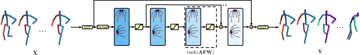
The detailed architecture of our generator is shown in Fig. 2. It consists of 4 residual blocks. Each block comprises 2 graph convolutional layers. It also contains two additional layers, one at the beginning, to bring the input to feature space, and the other at the end, to decode the feature to the residuals of the DCT coefficients.
7 Implementation Details
We implemented our network using Pytorch [44] and used ADAM [28] to train it. The learning rate was set to 0.001 with a decay rate defined by the function
| (5) |
where is the current epoch.
For Human3.6M, our model observes the past 25 frames to predict the future 100 frames, and we use the first 20 DCT coefficients. For HumanEva-I, our model predicts the future 60 frames given the past 15 frames, and we use the first 8 DCT coefficients.
To generate the pseudo ground truth for the multi-modal reconstruction error (), we follow the official DLow [57] implementation of the multi-modal version of FDE (MMFDE) and use the distance between the last pose of the history to choose the pseudo ground truth. That is, for a training sample, any other training sequence with similar last pose in terms of Euclidean distance is chosen to be a possible future. We set the distance threshold to 0.5 for both Human3.6M and HumanEva-I.
8 Additional Qualitative Results
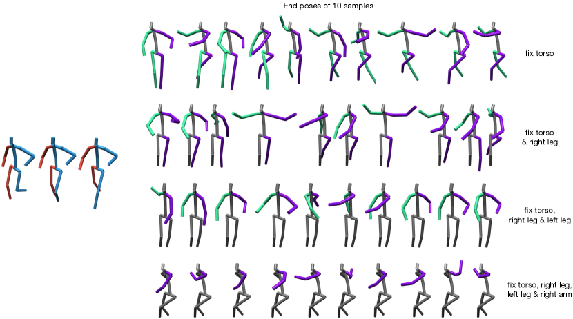
8.1 Controllable Motion Prediction with
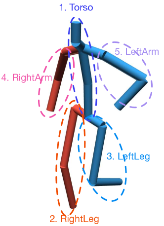
In the main paper, we divided a human pose into 2 parts (): lower body and upper body, and show the results of predicting motions with same lower body motion but diverse upper body motions. Here, we provide qualitative results with . In particular, as shown in Fig. 3, we split a pose into: 1. torso, 2. right leg, 3. left leg, 4. right arm and 5. left arm, following this order for prediction. As shown in Fig. 4, our model is able to perform different levels of controllable motion prediction given the detailed body parts segmentation.
8.2 Ablation Study
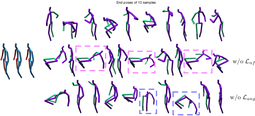
We show a qualitative comparison on the results of our model without either the pose prior loss or the angle loss in Fig. 5. This clearly demonstrates the dramatic decrease in pose quality in both cases.