This paper was converted on www.awesomepapers.org from LaTeX by an anonymous user.
Want to know more? Visit the Converter page.

Generalized Ribaucour-type surfaces

Milton Javier Cardenas Mendez
Instituto de Matemática e Estatística
Universidade Federal de Goiás, 74001-970 Goiânia, GO, Brazil
[email protected]
   Armardo Mauro Vasquez Corro
Instituto de Matemática e Estatística
Universidade Federal de Goiás, 74001-970 Goiânia, GO, Brazil
[email protected]
Abstract

In this work we generalize the surfaces studied in [8], we define the generalization of Ribaucour-type surfaces (in short, GRT-surfaces). We obtain present a representation for GRT-surfaces with prescribed Gauss map which depends on two holomorphic functions and a real function \ell. We give explicit examples of GRT-surfaces. Also, we use this representation to classify the GRT-surfaces of rotation.

Keywords.

Generalitation of Ribaucour-type surfaces, generalized Weingarten surfaces, prescribed normal Gauss map.

Introduction: Let Σ3\Sigma\subset\mathbb{R}^{3} be an oriented surface with normal Gauss map NN, functions Ψ,Λ:Σ3\Psi,\Lambda:\Sigma\rightarrow\mathbb{R}^{3} given by Ψ(p)=p,N(p)\Psi(p)=\langle p,N(p)\rangle and Λ(p)=p,p\Lambda(p)=\langle p,p\rangle, pΣp\in\Sigma, where ,\langle,\rangle denotes the Euclidean scalar product in 3\mathbb{R}^{3}, are called support function and quadratic distance function, respectively. Geometrically, Ψ(p)\Psi(p) measures the signed distance from the origin to TpMT_{p}M and Λ(p)\Lambda(p) measures the squared distance from the origin to pp. Let pΣp\in\Sigma, a sphere with center p+H(p)K(p)N(p)p+\frac{H(p)}{K(p)}N(p) and radius H(p)K(p)\frac{H(p)}{K(p)} is called the middle sphere.

In 1888, Appell [5] studied a class of surfaces oriented in 3\mathbb{R}^{3} associated with area-preserving sphere transformations. Later, Ferreira and Roitman [3] showed that these surfaces satisfy the Weingarten relation, H+ΨK=0H+\Psi K=0.

In 1907, Tzitzeica [9] studied hyperbolic surfaces oriented so that there is a nonzero constant cc\in\mathbb{R} for which K+c2Ψ4=0K+c^{2}\Psi^{4}=0.

In [1], the authors motivated by the works [5] and [9] defined generalized Weingarten surfaces as surfaces that satisfy a relation of the form A+BH+CK=0A+BH+CK=0, where A,B,C:ΣA,B,C:\Sigma\rightarrow\mathbb{R} are differentiable functions that do not depend on the parameterization of Σ\Sigma. In particular, they studied the class of surfaces that satisfy the relation 2ΨH+ΛK=02\Psi H+\Lambda K=0. Called Special Generalized Weingartem Surfaces depending on the support function and the distance function (in short, EDSGW-surfaces), these surfaces have the geometric property that all medium spheres pass through the origin. The authors obtained a Weierstrass-like representation of EDSGW-surfaces depending on two homomorphic functions. In [6], the authors classified isothermic EDSGW-surfaces in relation to the third fundamental shape parameterized by plane curvature lines. Also in [4], it is shown that EDSGW-surfaces are in correspondence with the surface class in 𝕊2×\mathbb{S}^{2}\times\mathbb{R} where the Gaussian curvature KK and the extrinsic curvature KEK_{E} satisfy K=2KEK=2K_{E}.

Martínez and Roitman, in [2] showed what appears to be the first example found for the second case of the problem posed by Élie Cartan in his classic book about external differential systems and their applications to Differential Geometry. Such examples are given by a class of Weingarten surfaces that satisfy the relation 2ΨH+(1+Λ)K=02\Psi H+(1+\Lambda)K=0, Ribaucour surface calls, these surfaces have the geometric property that all the medial spheres intercept a fixed sphere along a large circle.

In [10], the authors define a surface class called Ribaucour surface of harmonic type (in short, HR-surface) if it satisfies 2ΨH+(ce2μ+Λ)K=02\Psi H+(ce^{2\mu}+\Lambda)K=0, where cc is a nonzero real constant, μ\mu a harmonic function with respect to the third fundamental form. These surfaces generalize Ribaucour surfaces studied in [2].

Motivated by [8], we define Σ\Sigma be a surface with Gauss map NN is called a surface of type Ribaucour generalized or abbreviated GRT-Surface. There is a harmonic map μ\mu with respect to the third fundamental form and a function C:C:\mathbb{R}\rightarrow\mathbb{R} such that for all pΣp\in\Sigma the sphere with center p+(HC(μ)K+Ψ(2C(μ))2C(μ))N(p)p+\left(\frac{H}{C(\mu)K}+\frac{\Psi(2-C(\mu))}{2C(\mu)}\right)N(p) and radius (HC(μ)K+Ψ(2C(μ))2C(μ))\left(\frac{H}{C(\mu)K}+\frac{\Psi(2-C(\mu))}{2C(\mu)}\right), tangents a fixed sphere. In this case Σ\Sigma satisfies the following relation generalized Weingarten

HK=C(μ)(Λ2Ψ+Ψ2)Ψ.\frac{H}{K}=C(\mu)\left(\frac{-\Lambda}{2\Psi}+\frac{\Psi}{2}\right)-\Psi.

We obtain present a representation for GRT-surfaces with prescribed Gauss map which depends on two holomorphic functions and a real function \ell. We give explicit examples of GRT-surfaces. Also, we use this representation to classify the GRT-surfaces of rotation.

1 Preliminaries

In this section we fix the notation used in this work, Σ\Sigma a surface on 3\mathbb{R}^{3}, NN its normal Gaussian map, and UU an open subset of 2\mathbb{R}^{2}.

Let X:U2ΣX:U\subset\mathbb{R}^{2}\rightarrow\Sigma, a parameterization of a surface Σ\Sigma and N:U23N:U\subset\mathbb{R}^{2}\rightarrow\mathbb{R}^{3}, normal Gaussian map. Considering {X,1,X,2,N}\{X_{,1},X_{,2},N\} as a base of 3\mathbb{R}^{3}, where X,i(q)=Xui(q)X_{,i}(q)=\frac{\partial X}{\partial u_{i}}(q), 1i,j21\leq i,j\leq 2 further we can write vector X,ijX_{,ij}, 1i,j21\leq i,j\leq 2, as

X,ij=k=12Γ~ijkX,k+bijNX_{,ij}=\sum_{k=1}^{2}\widetilde{\Gamma}_{ij}^{k}X_{,k}+b_{ij}N

The Γ~ijk\widetilde{\Gamma}_{ij}^{k} coefficients are called Christoffel symbols.

Definition 1.1.

Let XX be a local parameterization of Σ\Sigma with map of Gauss NN, matrix W=(Wij)W=(W_{ij}), such that

N,i=j=12WijXj,1i2N_{,i}=\sum_{j=1}^{2}W_{ij}X_{j},\hskip 8.5359pt1\leq i\leq 2

is called the Weingarten matrix of Σ\Sigma.

Lemma 1.2.

Let NN be the normal Gaussian map given by (2) such that the metric Lij=N,i,N,jL_{ij}=\langle N_{,i},N_{,j}\rangle is Euclidean conformal. Christoffel’s symbols for metric LijL_{ij} are given by

Γijk=0,Γiii=Lii,i2Lii,Γiji=Lii,j2Lii,Γiii=Lii,j2Ljj\Gamma_{ij}^{k}=0,\hskip 8.5359pt\Gamma_{ii}^{i}=\frac{L_{ii,i}}{2L_{ii}},\hskip 8.5359pt\Gamma_{ij}^{i}=\frac{L_{ii,j}}{2L_{ii}},\hskip 8.5359pt\Gamma_{ii}^{i}=\frac{-L_{ii,j}}{2L_{jj}}

For i,ji,j e kk different.

Remark.

Let the inner product be defined by ,:×,f,g=f1g1+f2g2\langle,\rangle:\mathbb{C}\times\mathbb{C}\rightarrow\mathbb{R},\langle f,g\rangle=f_{1}g_{1}+f_{2}g_{2}, where f=f1+if2f=f_{1}+if_{2} and g=g1+ig2g=g_{1}+ig_{2} are holomorphic functions. If f,g,h:Uf,g,h:U\subset\mathbb{C}\rightarrow\mathbb{C} are holomorphic functions, then

f,g,1=f,g+f,gf,g,2=if,g+f,igfh,g=f,h¯gf=1,g+ii,fg,1=g,g,2=ig\begin{split}&\langle f,g\rangle_{,1}=\langle f^{\prime},g\rangle+\langle f,g^{\prime}\rangle\\ &\langle f,g\rangle_{,2}=\langle if^{\prime},g\rangle+\langle f,ig^{\prime}\rangle\\ &\langle fh,g\rangle=\langle f,\overline{h}g\rangle\\ &f=\langle 1,g\rangle+i\langle i,f\rangle\\ &g_{,1}=g^{\prime},g_{,2}=ig^{\prime}\\ \end{split} (1)

where f,g,1=f(z),g(z)u1\langle f,g\rangle_{,1}=\frac{\partial\langle f(z),g(z)\rangle}{\partial u_{1}}

Below we present some important results studied in [8].

Theorem 1.3.

Let Σ3\Sigma\subset\mathbb{R}^{3}, an orientable surface with non-zero Gauss-Kronecker curvature. Then there is a differentiable function h:Uh:U\rightarrow\mathbb{R} and gg a holomorphic function such that normal Gauss map is given by

N=(2g(u),1|g(u)|2)1+|g(u)|2N=\frac{(2g(u),1-|g(u)|^{2})}{1+|g(u)|^{2}} (2)

the coefficients of the IIIIII fundamental form are

Lij=4|g|2δij(1+|g|2)2L_{ij}=\frac{4|g^{\prime}|^{2}\delta_{ij}}{(1+|g|^{2})^{2}} (3)

Σ\Sigma is locally parameterized by

X(u)=j=12h(u),jLjjN(u),j+h(u)N(u)X(u)=\sum_{j=1}^{2}\frac{h(u)_{,j}}{L_{jj}}N(u)_{,j}+h(u)N(u) (4)

In this case h(u)=X(u),N(u)h(u)=\langle X(u),N(u)\rangle is the support function. Furthermore, the Weingarten matrix is given by W=V1W=V^{-1} where

Vij=1Lij(h,ijknh,kΓijk+hLijδij)V_{ij}=\frac{1}{L_{ij}}\left(h_{,ij}-\sum_{k}^{n}h_{,k}\Gamma_{ij}^{k}+hL_{ij}\delta_{ij}\right)

where Γijk\Gamma_{ij}^{k} are Christoffel’s symbols of NN and the fundamental forms II and IIII of XX, in local coordinates, are given by

I=X,i,X,j=k=1nVikVjkLkk,II=X,i,N,j=VijLjj.I=\langle X_{,i},X_{,j}\rangle=\sum_{k=1}^{n}V_{ik}V_{jk}L_{kk},\quad II=\langle X_{,i},N_{,j}\rangle=V_{ij}L_{jj}.

furthermore,

hL11+2h=2HK,\frac{\triangle h}{L_{11}}+2h=\frac{-2H}{K}, (5)
Λ(q)=X(q),X(q)=|Lh(q)|2+h(q)2\Lambda(q)=\langle X(q),X(q)\rangle=|\nabla_{L}h(q)|^{2}+h(q)^{2} (6)
Ψ(q)=X(q),N(q)=h(q)\Psi(q)=\langle X(q),N(q)\rangle=h(q)

called quadratic distance function and support function, respectively.

2 GRT-surfaces

In this chapter, we introduce a few classes of surfaces called surfaces. of generalized Ribaucour type and we call it GRT-surfaces, we show a local parameterization of this class of surfaces and characterize the case where such surfaces are rotating.

Definition 2.1.

Let Σ\Sigma be a surface with Gauss map NN is called a surface of type Ribaucour generalized or abbreviated GRT-Surface. There is a harmonic map μ\mu with respect to the third fundamental form and a function C:C:\mathbb{R}\rightarrow\mathbb{R} such that for all pΣp\in\Sigma the sphere with center p+(HC(μ)K+Ψ(2C(μ))2C(μ))N(p)p+\left(\frac{H}{C(\mu)K}+\frac{\Psi(2-C(\mu))}{2C(\mu)}\right)N(p) and radius (HC(μ)K+Ψ(2C(μ))2C(μ))\left(\frac{H}{C(\mu)K}+\frac{\Psi(2-C(\mu))}{2C(\mu)}\right), tangents a fixed sphere. In this case Σ\Sigma satisfies the following relation generalized Weingarten

HK=C(μ)(Λ2Ψ+Ψ2)Ψ.\frac{H}{K}=C(\mu)\left(\frac{-\Lambda}{2\Psi}+\frac{\Psi}{2}\right)-\Psi. (7)
Remark.

We show particular cases of GRT-surfaces for different values of CC.

  1. 1.

    If C(t)=0C(t)=0 then

    HK=C(t)(Λ2Ψ+Ψ2)Ψ=Ψ\frac{H}{K}=C(t)\left(\frac{-\Lambda}{2\Psi}+\frac{\Psi}{2}\right)-\Psi=-\Psi
    H+ΨK=0.H+\Psi K=0.

    These are the Appell surfaces associated with area-preserving transformations on the sphere, studied by Ferreira and Roitman in [3].

  2. 2.

    If C(t)=1C(t)=1 then

    HK=C(t)(Λ2Ψ+Ψ2)Ψ=Λ2Ψ+Ψ2Ψ=Λ2ΨΨ2.\frac{H}{K}=C(t)\left(\frac{-\Lambda}{2\Psi}+\frac{\Psi}{2}\right)-\Psi=\frac{-\Lambda}{2\Psi}+\frac{\Psi}{2}-\Psi=-\frac{\Lambda}{2\Psi}-\frac{\Psi}{2}.

    They are TR-surfaces studied in [8]

Lemma 2.2.

Consider holomorphic functions g:g:\mathbb{C}\rightarrow\mathbb{C}_{\infty} and f:Σf:\Sigma\rightarrow\mathbb{C}, with g0g^{\prime}\neq 0, where Σ\Sigma is a Riemann surface. Taking the local parameters z=u1+iu2Σz=u_{1}+iu_{2}\in\Sigma and μ=1,f\mu=\langle 1,f\rangle such that h=(μ)h=\ell(\mu), the matrix

Vij=1Ljj(h,ijk=12h,kΓijk+hLijδij),1i,j2.V_{ij}=\frac{1}{L_{jj}}\left(h_{,ij}-\sum_{k=1}^{2}h_{,k}\Gamma_{ij}^{k}+hL_{ij}\delta_{ij}\right),\hskip 11.38092pt1\leq i,j\leq 2.

Using the metric given by (3), we have

V11=T24|g|2[′′(μ)1,f2(μ)1,ξ]+(μ),V12=V21=T24|g|2[′′(μ)1,if22+(μ)i,ξ],V22=T24|g|2[′′(μ)1,if2+(μ)1,ξ]+(μ).\begin{split}&V_{11}=\frac{T^{2}}{4|g^{\prime}|^{2}}[\ell^{\prime\prime}(\mu)\langle 1,f^{\prime}\rangle^{2}-\ell^{\prime}(\mu)\langle 1,\xi\rangle]+\ell(\mu),\\ &V_{12}=V_{21}=\frac{T^{2}}{4|g^{\prime}|^{2}}\left[\ell^{\prime\prime}(\mu)\left\langle 1,\frac{if^{\prime 2}}{2}\right\rangle+\ell^{\prime}(\mu)\langle i,\xi\rangle\right],\\ &V_{22}=\frac{T^{2}}{4|g^{\prime}|^{2}}[\ell^{\prime\prime}(\mu)\langle 1,if^{\prime}\rangle^{2}+\ell^{\prime}(\mu)\langle 1,\xi\rangle]+\ell(\mu).\end{split} (8)

Here ξ=f(g′′g2Tgg¯)f′′\xi=f^{\prime}\left(\frac{g^{\prime\prime}}{g^{\prime}}-\frac{2}{T}g^{\prime}\overline{g}\right)-f^{\prime\prime}, furthermore, trace of VV give for

trV=′′(μ)|f|2T24|g|2+2(μ).trV=\frac{\ell^{\prime\prime}(\mu)|f^{\prime}|^{2}T^{2}}{4|g^{\prime}|^{2}}+2\ell(\mu).
Proof.

Let h=(μ)=(1,f)h=\ell(\mu)=\ell(\langle 1,f\rangle), the derivatives of hh are given by:

h,1=(μ)1,fh,11=′′(μ)1,f2+(μ)1,f′′h,2=(μ)1,ifh,22=′′(μ)1,if2(μ)1,f′′h,12=′′(μ)1,if1,f+(μ)1,if′′.\begin{split}&h_{,1}=\ell^{\prime}(\mu)\langle 1,f^{\prime}\rangle\\ &h_{,11}=\ell^{\prime\prime}(\mu)\langle 1,f^{\prime}\rangle^{2}+\ell^{\prime}(\mu)\langle 1,f^{\prime\prime}\rangle\\ &h_{,2}=\ell^{\prime}(\mu)\langle 1,if^{\prime}\rangle\\ &h_{,22}=\ell^{\prime\prime}(\mu)\langle 1,if^{\prime}\rangle^{2}-\ell^{\prime}(\mu)\langle 1,f^{\prime\prime}\rangle\\ &h_{,12}=\ell^{\prime\prime}(\mu)\langle 1,if^{\prime}\rangle\langle 1,f^{\prime}\rangle+\ell^{\prime}(\mu)\langle 1,if^{\prime\prime}\rangle.\end{split}

Using the Christoffel symbols found in Lemma 1.2, we can infer that

Γ111=Tg,g′′2|g|2g,gT|g|2,\Gamma_{11}^{1}=\frac{T\langle g^{\prime},g^{\prime\prime}\rangle-2|g^{\prime}|^{2}\langle g,g^{\prime}\rangle}{T|g^{\prime}|^{2}},
Γ222=Tg,ig′′2|g|2g,igT|g|2,\Gamma_{22}^{2}=\frac{T\langle g^{\prime},ig^{\prime\prime}\rangle-2|g^{\prime}|^{2}\langle g,ig^{\prime}\rangle}{T|g^{\prime}|^{2}},
Γ112=2|g|2g,igTg,ig′′T|g|2,\Gamma_{11}^{2}=\frac{2|g^{\prime}|^{2}\langle g,ig^{\prime}\rangle-T\langle g^{\prime},ig^{\prime\prime}\rangle}{T|g^{\prime}|^{2}},
Γ221=2|g|2g,gTg,g′′T|g|2.\Gamma_{22}^{1}=\frac{2|g^{\prime}|^{2}\langle g,g^{\prime}\rangle-T\langle g^{\prime},g^{\prime\prime}\rangle}{T|g^{\prime}|^{2}}.

Using the previous expressions and (1) we have

k=12Γ11kh,k=Γ111h,1+Γ112h,2=(μ)1,f[Tg,g′′2|g|2g,gT|g|2](μ)i,f[2|g|2g,igTg,ig′′T|g|2]=(μ)1,f+ii,f,g,g′′|g|22Tg,g+i(g,ig′′|g|22Tg,ig)=(μ)f,g,g′′|g|2+ig,ig′′|g|22T(g,g+ig,ig)=(μ)f,g′′¯g|g|22Tg¯g=(μ)f,(g′′g)¯2Tg¯g=(μ)f,g′′g2Tg¯g¯=(μ)1,f(g′′g2Tgg¯)=(μ)1,ξ+f′′,\begin{split}\sum_{k=1}^{2}\Gamma_{11}^{k}h_{,k}&=\Gamma_{11}^{1}h_{,1}+\Gamma_{11}^{2}h_{,2}\\ &=\ell^{\prime}(\mu)\langle 1,f^{\prime}\rangle\left[\frac{T\langle g^{\prime},g^{\prime\prime}\rangle-2|g^{\prime}|^{2}\langle g,g^{\prime}\rangle}{T|g^{\prime}|^{2}}\right]\\ &-\ell^{\prime}(\mu)\langle i,f^{\prime}\rangle\left[\frac{2|g^{\prime}|^{2}\langle g,ig^{\prime}\rangle-T\langle g^{\prime},ig^{\prime\prime}\rangle}{T|g^{\prime}|^{2}}\right]\\ &=\ell^{\prime}(\mu)\left\langle\langle 1,f^{\prime}\rangle+i\langle i,f^{\prime}\rangle,\frac{\langle g^{\prime},g^{\prime\prime}\rangle}{|g^{\prime}|^{2}}-\frac{2}{T}\langle g,g^{\prime}\rangle+i\left(\frac{\langle g^{\prime},ig^{\prime\prime}\rangle}{|g^{\prime}|^{2}}-\frac{2}{T}\langle g,ig^{\prime}\rangle\right)\right\rangle\\ &=\ell^{\prime}(\mu)\left\langle f^{\prime},\frac{\langle g^{\prime},g^{\prime\prime}\rangle}{|g^{\prime}|^{2}}+i\frac{\langle g^{\prime},ig^{\prime\prime}\rangle}{|g^{\prime}|^{2}}-\frac{2}{T}(\langle g,g^{\prime}\rangle+i\langle g,ig^{\prime}\rangle)\right\rangle\\ &=\ell^{\prime}(\mu)\left\langle f^{\prime},\frac{\bar{g^{\prime\prime}}g^{\prime}}{|g^{\prime}|^{2}}-\frac{2}{T}\bar{g^{\prime}}g\right\rangle=\ell^{\prime}(\mu)\left\langle f^{\prime},\overline{\left(\frac{g^{\prime\prime}}{g^{\prime}}\right)}-\frac{2}{T}\overline{g^{\prime}}g\right\rangle\\ &=\ell^{\prime}(\mu)\left\langle f^{\prime},\overline{\frac{g^{\prime\prime}}{g^{\prime}}-\frac{2}{T}\overline{g}g^{\prime}}\right\rangle=\ell^{\prime}(\mu)\left\langle 1,f^{\prime}\left(\frac{g^{\prime\prime}}{g^{\prime}}-\frac{2}{T}g^{\prime}\overline{g}\right)\right\rangle\\ &=\ell^{\prime}(\mu)\langle 1,\xi+f^{\prime\prime}\rangle,\end{split}

where ξ=f(g′′g2Tgg¯)f′′\xi=f^{\prime}\left(\frac{g^{\prime\prime}}{g^{\prime}}-\frac{2}{T}g^{\prime}\overline{g}\right)-f^{\prime\prime}. Similarly, knowing that Γ211=Γ222,Γ122=Γ111\Gamma_{21}^{1}=\Gamma_{22}^{2},\Gamma_{12}^{2}=\Gamma_{11}^{1}, we obtain

k=12Γ22kh,k=(μ)1,ξ+f′′,\sum_{k=1}^{2}\Gamma_{22}^{k}h_{,k}=-\ell^{\prime}(\mu)\langle 1,\xi+f^{\prime\prime}\rangle,

It is

k=12Γ12kh,k=(μ)i,ξ+f′′.\sum_{k=1}^{2}\Gamma_{12}^{k}h_{,k}=-\ell^{\prime}(\mu)\langle i,\xi+f^{\prime\prime}\rangle.

So we can write

V11=1L11(h,11k=12Γ11kh,k+hL11)=T24|g|2[′′(μ)1,f2+(μ)1,f′′(μ)1,ξ+f′′]+(μ)=T24|g|2[′′(μ)1,f2+(μ)[1,f′′1,ξ+f′′]]+(μ)=T24|g|2[′′(μ)1,f2(μ)1,xi]+(μ)\begin{split}V_{11}&=\frac{1}{L_{11}}\left(h_{,11}-\sum_{k=1}^{2}\Gamma_{11}^{k}h_{,k}+hL_{11}\right)\\ &=\frac{T^{2}}{4|g^{\prime}|^{2}}[\ell^{\prime\prime}(\mu)\langle 1,f^{\prime}\rangle^{2}+\ell^{\prime}(\mu)\langle 1,f^{\prime\prime}\rangle-\ell^{\prime}(\mu)\langle 1,\xi+f^{\prime\prime}\rangle]+\ell(\mu)\\ &=\frac{T^{2}}{4|g^{\prime}|^{2}}[\ell^{\prime\prime}(\mu)\langle 1,f^{\prime}\rangle^{2}+\ell^{\prime}(\mu)[\langle 1,f^{\prime\prime}\rangle-\langle 1,\xi+f^{\prime\prime}\rangle]]+\ell(\mu)\\ &=\frac{T^{2}}{4|g^{\prime}|^{2}}[\ell^{\prime\prime}(\mu)\langle 1,f^{\prime}\rangle^{2}-\ell^{\prime}(\mu)\langle 1,\ xi\rangle]+\ell(\mu)\end{split}
V22=1L22(h,22k=12Γ22kh,k+hL22)=T24|g|2[′′(μ)1,if2+(μ)1,xi]+(μ)\begin{split}V_{22}&=\frac{1}{L_{22}}\left(h_{,22}-\sum_{k=1}^{2}\Gamma_{22}^{k}h_{,k}+hL_{22}\right)\\ &=\frac{T^{2}}{4|g^{\prime}|^{2}}[\ell^{\prime\prime}(\mu)\langle 1,if^{\prime}\rangle^{2}+\ell^{\prime}(\mu)\langle 1,\ xi\rangle]+\ell(\mu)\end{split}
V12=1L22(h,12k=12Γ12kh,k)=T24|g|2[′′(μ)1,if22+(μ)i,ξ].\begin{split}V_{12}&=\frac{1}{L_{22}}\left(h_{,12}-\sum_{k=1}^{2}\Gamma_{12}^{k}h_{,k}\right)\\ &=\frac{T^{2}}{4|g^{\prime}|^{2}}\left[\ell^{\prime\prime}(\mu)\left\langle 1,\frac{if^{\prime 2}}{2}\right\rangle+\ell^{\prime}(\mu)\langle i,\xi\rangle\right].\end{split}

Thus,

trV=V11+V22=T24|g|2[′′(μ)(1,f2+1,if2)]+2(μ)\begin{split}trV&=V_{11}+V_{22}\\ &=\frac{T^{2}}{4|g^{\prime}|^{2}}[\ell^{\prime\prime}(\mu)(\langle 1,f^{\prime}\rangle^{2}+\langle 1,if^{\prime}\rangle^{2})]+2\ell(\mu)\end{split}

therefore,

trV=′′(μ)|f|2T24|g|2+2(μ).trV=\frac{\ell^{\prime\prime}(\mu)|f^{\prime}|^{2}T^{2}}{4|g^{\prime}|^{2}}+2\ell(\mu).

Theorem 2.3.

Let XX be given by (4), C:C:\mathbb{R}\rightarrow\mathbb{R} and μ:2\mu:\mathbb{R}^{2}\rightarrow\mathbb{R}, μ\mu harmonic with respect to third fundamental form then XX is a TRG-surface if and only if

hLhC(μ)|Lh|2=0.h\triangle_{L}h-C(\mu)|\nabla_{L}h|^{2}=0. (9)
Proof.

Using the equation (5) we have

HK=12(Lh+2h).\frac{H}{K}=-\frac{1}{2}(\triangle_{L}h+2h). (10)

Using (7) and (10), we get the following equivalence

12(Lh+2h)=C(μ)(Λ2Ψ+Ψ2)Ψ=C(μ)2Ψ(Λ+Ψ2)Ψ-\frac{1}{2}(\triangle_{L}h+2h)=C(\mu)\left(\frac{-\Lambda}{2\Psi}+\frac{\Psi}{2}\right)-\Psi=\frac{C(\mu)}{2\Psi}(-\Lambda+\Psi^{2})-\Psi
Lh+2h=C(μ)Ψ(Λ+Ψ2)+2Ψ,\Leftrightarrow\triangle_{L}h+2h=-\frac{C(\mu)}{\Psi}(-\Lambda+\Psi^{2})+2\Psi,

remembering that h=Ψh=\Psi, we arrive at

hLh=C(μ)(ΛΨ2),h\triangle_{L}h=C(\mu)(\Lambda-\Psi^{2}),

by (6) we get

hLh=C(μ)(|Lh|2+Ψ2Ψ2),h\triangle_{L}h=C(\mu)(|\nabla_{L}h|^{2}+\Psi^{2}-\Psi^{2}),

logo hLhC(μ)|Lh|2=0h\triangle_{L}h-C(\mu)|\nabla_{L}h|^{2}=0. ∎

The following theorem allows to obtain a class of GRT-surfaces.

Theorem 2.4.

Let Σ\Sigma be a Riemann surface and X:Σ3X:\Sigma\rightarrow\mathbb{R}^{3} be an immersion such that the Gauss-kronecker curvature is non-zero. Let :\ell:\mathbb{R}\rightarrow\mathbb{R} and μ=1,f\mu=\langle 1,f\rangle, with ff a holomorphic function and h=(μ)h=\ell(\mu) . Then XX is given by (4) and is a TRG-surface with C=′′()2C=\frac{\ell\ell^{\prime\prime}}{(\ell^{\prime})^{2}}, where 0\ell^{\prime}\neq 0. Furthermore, let gg be a holomorphic function and g0g^{\prime}\neq 0, then X(Σ)X(\Sigma) is locally parameterized by

X=(μ)2|g|2(Tgf¯2gg,gf,2g,gf)+(μ)(2g,2T)T,X=\frac{\ell^{\prime}(\mu)}{2|g^{\prime}|^{2}}(Tg^{\prime}\bar{f^{\prime}}-2g\langle g^{\prime},gf^{\prime}\rangle,-2\langle g^{\prime},gf^{\prime}\rangle)+\ell(\mu)\frac{(2g,2-T)}{T}, (11)

with T=1+|g|2T=1+|g|^{2}.

Proof.

Let h(μ)=(μ)h(\mu)=\ell(\mu) where \ell be a real function and μ=1,f\mu=\langle 1,f\rangle, in this case we have,

h,1=(μ)μ,1andh,2=(μ)μ,2h_{,1}=\ell^{\prime}(\mu)\mu_{,1}\hskip 11.38092ptand\hskip 11.38092pth_{,2}=\ell^{\prime}(\mu)\mu_{,2}
h,11=′′(μ)(μ,12+μ,11)andh,22=′′(μ)(μ,22+μ,22).h_{,11}=\ell^{\prime\prime}(\mu)(\mu_{,1}^{2}+\mu_{,11})\hskip 11.38092ptand\hskip 11.38092pth_{,22}=\ell^{\prime\prime}(\mu)(\mu_{,2}^{2}+\mu_{,22}).

Substituting the above derivatives in (9) we have the following equivalence

(μ)(′′(μ)(μ,12+μ,22)+(μ)(μ,11+μ,22))C(μ)(2(μ)(μ,12+μ,22))=0\ell(\mu)(\ell^{\prime\prime}(\mu)(\mu_{,1}^{2}+\mu_{,2}^{2})+\ell^{\prime}(\mu)(\mu_{,11}+\mu_{,22}))-C(\mu)(\ell^{\prime 2}(\mu)(\mu_{,1}^{2}+\mu_{,2}^{2}))=0
(μ)′′(μ)|Lμ|2=C(μ)2(μ)|Lμ|2.\Leftrightarrow\ell(\mu)\ell^{\prime\prime}(\mu)|\nabla_{L}\mu|^{2}=C(\mu)\ell^{\prime 2}(\mu)|\nabla_{L}\mu|^{2}.

Therefore

C(μ)=(μ)′′(μ)2(μ).C(\mu)=\frac{\ell(\mu)\ell^{\prime\prime}(\mu)}{\ell^{\prime 2}(\mu)}.

On the other hand, we can write (4) as

X(u)=j=12h,jLjjN,j+hN=1L11[h,1N,1+h,2N,2]+hN=T24|g|2[(1,f)1,f2T2(Tg,12gg,g,2g,g)]+T24|g|2[(1,f)1,if2T2(Tg,22gg,ig,2g,ig)]+(1,f)(2g,2T)T=(1,f)2|g|2(Tgf¯2gg,gf,2g,gf)+(1,f)(2g,2T)T.\begin{split}X(u)&=\sum_{j=1}^{2}\frac{h_{,j}}{L_{jj}}N_{,j}+hN=\frac{1}{L_{11}}[h_{,1}N_{,1}+h_{,2}N_{,2}]+hN\\ &=\frac{T^{2}}{4|g^{\prime}|^{2}}\left[\ell^{\prime}(\langle 1,f\rangle)\langle 1,f^{\prime}\rangle\frac{2}{T^{2}}(Tg_{,1}-2g\langle g^{\prime},g\rangle,-2\langle g^{\prime},g\rangle)\right]\\ &+\frac{T^{2}}{4|g^{\prime}|^{2}}\left[\ell^{\prime}(\langle 1,f\rangle)\langle 1,if^{\prime}\rangle\frac{2}{T^{2}}(Tg_{,2}-2g\langle g,ig^{\prime}\rangle,-2\langle g,ig^{\prime}\rangle)\right]+\ell(\langle 1,f\rangle)\frac{(2g,2-T)}{T}\\ &=\frac{\ell^{\prime}(\langle 1,f\rangle)}{2|g^{\prime}|^{2}}(Tg^{\prime}\bar{f^{\prime}}-2g\langle g^{\prime},gf^{\prime}\rangle,-2\langle g^{\prime},gf^{\prime}\rangle)+\ell(\langle 1,f\rangle)\frac{(2g,2-T)}{T}.\end{split}

Remark.

The coefficients of the first and second fundamental forms of XX and using (8) are given by:

E=X,1,X,1=V11N,1+V12N,2,V11N,1+V12N,2=V112L11+V122L22=(V112+V122)L11=T24|g|2[′′2(μ)(1,f4+1,if222)2′′(1,f21,ξ1,if2i,ξ)+2(μ)|ξ|2]+2[′′(μ)1,f2(μ)1,ξ]+42(μ)|g|2T2,\begin{split}E&=\langle X_{,1},X_{,1}\rangle=\langle V_{11}N_{,1}+V_{12}N_{,2},V_{11}N_{,1}+V_{12}N_{,2}\rangle\\ &=V_{11}^{2}L_{11}+V_{12}^{2}L_{22}=(V_{11}^{2}+V_{12}^{2})L_{11}\\ &=\frac{T^{2}}{4|g^{\prime}|^{2}}[\ell^{\prime\prime 2}(\mu)\left(\langle 1,f^{\prime}\rangle^{4}+\left\langle 1,\frac{if^{\prime 2}}{2}\right\rangle^{2}\right)-2\ell^{\prime\prime}\ell^{\prime}\left(\langle 1,f^{\prime}\rangle^{2}\langle 1,\xi\rangle-\left\langle 1,\frac{if^{\prime}}{2}\right\rangle\langle i,\xi\rangle\right)\\ &+\ell^{\prime 2}(\mu)|\xi|^{2}]+2\ell[\ell^{\prime\prime}(\mu)\langle 1,f^{\prime}\rangle^{2}-\ell^{\prime}(\mu)\langle 1,\xi\rangle]+\frac{4\ell^{2}(\mu)|g^{\prime}|^{2}}{T^{2}},\end{split}
F=X,1,X,2=V11N,1+V12N,2,V21N,1+V22N,2=V11V21L11+V12V22L22=(V11+V22)V12L11=[′′(μ)|f|2T24|g|2+2(μ)]][′′(μ)1,if22+(μ)i,ξ],\begin{split}F&=\langle X_{,1},X_{,2}\rangle=\langle V_{11}N_{,1}+V_{12}N_{,2},V_{21}N_{,1}+V_{22}N_{,2}\rangle\\ &=V_{11}V_{21}L_{11}+V_{12}V_{22}L_{22}=(V_{11}+V_{22})V_{12}L_{11}\\ &=\left[\frac{\ell^{\prime\prime}(\mu)|f^{\prime}|^{2}T^{2}}{4|g^{\prime}|^{2}}+2\ell(\mu)]\right]\left[\ell^{\prime\prime}(\mu)\left\langle 1,\frac{if^{\prime 2}}{2}\right\rangle+\ell^{\prime}(\mu)\langle i,\xi\rangle\right],\end{split}
G=X,2,X,2=V21N,1+V22N,2,V21N,1+V22N,2=V212L11+V222L22=V222L22+V212L11=(V222+V212)L11=T24|g|2[′′2(μ)(1,if4+1,if222)+2′′(1,if21,ξ+1,if22i,ξ)+2(μ)|ξ|2]+2[′′(μ)1,if2+(μ)1,ξ]+42(μ)|g|2T2,\begin{split}G&=\langle X_{,2},X_{,2}\rangle=\langle V_{21}N_{,1}+V_{22}N_{,2},V_{21}N_{,1}+V_{22}N_{,2}\rangle=V_{21}^{2}L_{11}+V_{22}^{2}L_{22}\\ &=V_{22}^{2}L_{22}+V_{21}^{2}L_{11}=(V_{22}^{2}+V_{21}^{2})L_{11}\\ &=\frac{T^{2}}{4|g^{\prime}|^{2}}[\ell^{\prime\prime 2}(\mu)\left(\langle 1,if^{\prime}\rangle^{4}+\left\langle 1,\frac{if^{\prime 2}}{2}\right\rangle^{2}\right)+2\ell^{\prime\prime}\ell^{\prime}\left(\langle 1,if^{\prime}\rangle^{2}\langle 1,\xi\rangle+\left\langle 1,\frac{if^{\prime 2}}{2}\right\rangle\langle i,\xi\rangle\right)\\ &+\ell^{\prime 2}(\mu)|\xi|^{2}]+2\ell[\ell^{\prime\prime}(\mu)\langle 1,if^{\prime}\rangle^{2}+\ell^{\prime}(\mu)\langle 1,\xi\rangle]+\frac{4\ell^{2}(\mu)|g^{\prime}|^{2}}{T^{2}},\end{split}
e=X,1,N,1=V11N,1+V12N,2,N,1=V11L11=′′(μ)1,f2(μ)1,ξ+4(μ)|g|2T2,\begin{split}e&=\langle X_{,1},N_{,1}\rangle=\langle V_{11}N_{,1}+V_{12}N_{,2},N_{,1}\rangle=V_{11}L_{11}\\ &=\ell^{\prime\prime}(\mu)\langle 1,f^{\prime}\rangle^{2}-\ell^{\prime}(\mu)\langle 1,\xi\rangle+\frac{4\ell(\mu)|g^{\prime}|^{2}}{T^{2}},\end{split}
f=X,1,N,2=V11N,1+V12N,2,N,2=V12L22=′′(μ)1,if22+(μ)i,ξ,\begin{split}f&=\langle X_{,1},N_{,2}\rangle=\langle V_{11}N_{,1}+V_{12}N_{,2},N_{,2}\rangle=V_{12}L_{22}\\ &=\ell^{\prime\prime}(\mu)\left\langle 1,\frac{if^{\prime 2}}{2}\right\rangle+\ell^{\prime}(\mu)\langle i,\xi\rangle,\end{split}
g=X,2,N,2=V21N,1+V22N,2,N,2=V22L22=′′(μ)1,if2+(μ)1,ξ+4(μ)|g|2T2.\begin{split}g&=\langle X_{,2},N_{,2}\rangle=\langle V_{21}N_{,1}+V_{22}N_{,2},N_{,2}\rangle=V_{22}L_{22}\\ &=\ell^{\prime\prime}(\mu)\langle 1,if^{\prime}\rangle^{2}+\ell^{\prime}(\mu)\langle 1,\xi\rangle+\frac{4\ell(\mu)|g^{\prime}|^{2}}{T^{2}}.\end{split}

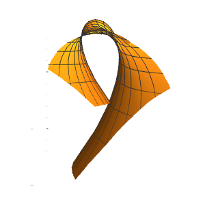
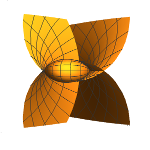
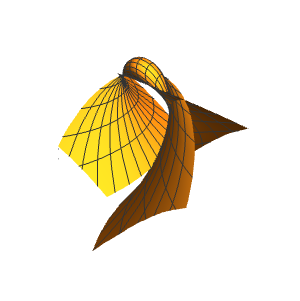
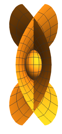
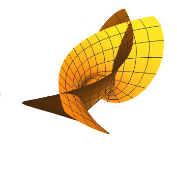
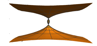
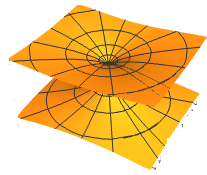
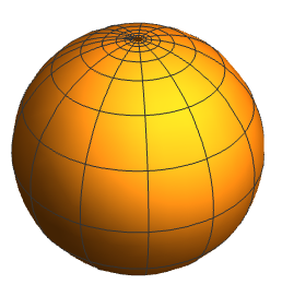
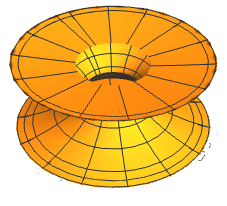
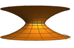
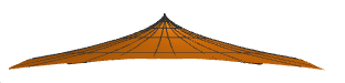
The following examples are GRT-surfaces for some holomorphic functions ff and gg with z=u1+iu2z=u_{1}+iu_{2}\in\mathbb{C}, using (11) we have

Refer to caption
Refer to caption
Refer to caption
Figure 1: (t)=t2+t+1\ell(t)=t^{2}+t+1,  f(z)=g(z)=z=u1+iu2f(z)=g(z)=z=u_{1}+iu_{2}
Refer to caption
Refer to caption
Refer to caption
Figure 2: (t)=cos(t)\ell(t)=\cos(t),  f(z)=g(z)=z=u1+iu2f(z)=g(z)=z=u_{1}+iu_{2}

The following results will be used to classify the GRT-surfaces given by (11).

Lemma 2.5.

Let Σn+1\Sigma\subset\mathbb{R}^{n+1} be an orientable hypersurface with non-zero Gauss-Kronecker curvature. Then there exists a differentiable function h:Uh:U\rightarrow\mathbb{R} such that the normal Gaussian map is given by (2) and Σ\Sigma is locally parameterized by (4). Then X(U)X(U) is rotational if and only if h is a radial function.

Proof.

If X(U)X(U) is rotational, without loss of generality, we can assume that the axis of rotation is the xn+1x_{n+1} axis. This way, the sections orthogonal to the axis of rotation determine in X(U)X(U) spheres (n1)(n-1) dimensional centered on this axis. Note that along these spheres both |X|2|X|^{2} and the angle between XX and NN are constant. Given that

X,N=h,X,X=|Lh|2+h2,Lij=N,i,N,j.\langle X,N\rangle=h,\quad\langle X,X\rangle=|\nabla_{L}h|^{2}+h^{2},\quad L_{ij}=\langle N_{,i},N_{,j}\rangle.

We conclude that hh and |Lh|2|\nabla_{L}h|^{2} are constant along these spheres. Taking NN as the inverse of the stereographic projection we get,

Lij=4δij(1+|u|2)2,L_{ij}=\frac{4\delta_{ij}}{(1+|u|^{2})^{2}},

so that,

|Lh|2=(1+|u|22)2|h|,|\nabla_{L}h|^{2}=\left(\frac{1+|u|^{2}}{2}\right)^{2}|\nabla h|,

which says that |u|2|u|^{2} is constant as one traverses the orthogonal sections, therefore hh is constant along the spheres (n1)(n-1) dimensional centered at the origin, therefore hh is a function radial.

Let hh be a radial function, we write h(u)=J(|u|2)h(u)=J(|u|^{2}), uUu\in U for JJ a differentiable function. Let |u|2=t|u|^{2}=t and denote the derivative of JJ with respect to tt as J(t)J^{\prime}(t). Thus, h,i=2Juih_{,i}=2J^{\prime}u_{i} and taking NN as the inverse of the stereographic projection we have,

X=((J(1t)+2J1+t)u,2tJ+J(1t1+t)).X=\left((J^{\prime}(1-t)+\frac{2J}{1+t})u,-2tJ^{\prime}+J(\frac{1-t}{1+t})\right).

If 2tJ+J(1t1+t)-2tJ^{\prime}+J(\frac{1-t}{1+t}) is constant then

|(J(1t)+2J1+t)u|2=((J(1t)+2J1+t))2t.\left|(J^{\prime}(1-t)+\frac{2J}{1+t})u\right|^{2}=\left((J^{\prime}(1-t)+\frac{2J}{1+t})\right)^{2}t.

Which means that the sections orthogonal to the axis xn+1x_{n+1} determine in X(U)X(U) spheres (n1)(n-1) dimensional centered on this axis, so that X(U)X(U) is of rotation . ∎

Theorem 2.6.

Let Σ\Sigma be a GRT-surface given by (11), connected, where \ell is a real function and μ=1,f\mu=\langle 1,f\rangle. Then Σ\Sigma is rotational if and only if, there are constants a,ba,b\in\mathbb{R}, such that Σ\Sigma can be locally parameterized by

Xab(u1,u2)=(M(u1)cos(u2),M(u1)sin(u2),N(u1)),X_{ab}(u_{1},u_{2})=\left(M(u_{1})\cos(u_{2}),M(u_{1})\sin(u_{2}),N(u_{1})\right),
M(u1)=11+e2u1[a(μ)(eu1e3u1)+4ell(μ)eu12]M(u_{1})=\frac{1}{1+e^{2u_{1}}}\left[\frac{a\ell^{\prime}(\mu)(e^{-u_{1}}-e^{3u_{1}})+4\ ell(\mu)e^{u_{1}}}{2}\right]

and

N(u1)=11+e2u1[(μ)(1e2u1)a(μ)(1+e2u1)].N(u_{1})=\frac{1}{1+e^{2u_{1}}}\left[\ell(\mu)(1-e^{2u_{1}})-a\ell^{\prime}(\mu)(1+e^{2u_{1}})\right].
Proof.

From Theorem 2.4, we have that Σ\Sigma is locally parameterized by

X=(μ)2|g|2(Tgf¯2gg,gf,2g,gf)+(μ)(2g,2T)T,X=\frac{\ell^{\prime}(\mu)}{2|g^{\prime}|^{2}}(Tg^{\prime}\bar{f^{\prime}}-2g\langle g^{\prime},gf^{\prime}\rangle,-2\langle g^{\prime},gf^{\prime}\rangle)+\ell(\mu)\frac{(2g,2-T)}{T},

where f,gf,g are holomorphic functions, \ell is not constant and remembering that h=(μ)h=\ell(\mu), h,2=(μ)1,if=0h,_{2}=\ell^{\prime}(\mu)\langle 1,if^{\prime}\rangle=0 and 1,if=0\langle 1,if^{\prime}\rangle=0. The Cauchy-Riemann equations guarantee us that f(z)=az+z0f(z)=az+z_{0}, with z=u1+iu2,z0=b+icz=u_{1}+iu_{2},z_{0}=b+ic\in\mathbb{C}, thus Thus, by the lemma 2.5 we have that Σ\Sigma is rotational if and only if

g(z)=ez,h(z)=(au1+b),g(z)=e^{z},\hskip 5.69046pth(z)=\ell(au_{1}+b),

so that f(z)=af^{\prime}(z)=a, g(z)=g(z)g^{\prime}(z)=g(z) and T=1+e2u1T=1+e^{2u_{1}}. In this conditions,

X=(μ)2|g|2(Tgf¯2gg,gf,2g,gf)+(μ)(2g,2T)T=(μ)2eu1((1+e2u1)eza2ezez,eza,2ez,eza)+(μ)(2ez1+e2u1,1e2u11+e2u1)=(μ)2e2u1((a+ae2u1)ez2ae2u1ez,2ae2u1)+(μ)(2ez1+e2u1,1e2u11+e2u1)=(μ)2e2u1((aae2u1)ez,2ae2u1)+(μ)(2ez1+e2u1,1e2u11+e2u1)=(μ)(aez(e2u11)2,a)+(μ)(2ez1+e2u1,1e2u11+e2u1)=((μ)aez(e2u11)2,(μ)a)+(2(μ)ez1+e2u1,(μ)(1e2u1)1+e2u1)=((a(μ)(eu1eu1)2+2(μ)eu11+e2u1)(cos(u2)+isin(u2)),(μ)(1e2u1)1+e2u1a(μ)).\begin{split}X&=\frac{\ell^{\prime}(\mu)}{2|g^{\prime}|^{2}}(Tg^{\prime}\bar{f^{\prime}}-2g\langle g^{\prime},gf^{\prime}\rangle,-2\langle g^{\prime},gf^{\prime}\rangle)+\ell(\mu)\frac{(2g,2-T)}{T}\\ &=\frac{\ell^{\prime}(\mu)}{2e^{u_{1}}}\left((1+e^{2u_{1}})e^{z}a-2e^{z}\langle e^{z},e^{z}a\rangle,-2\langle e^{z},e^{z}a\rangle\right)+\ell(\mu)\left(\frac{2e^{z}}{1+e^{2u_{1}}},\frac{1-e^{2u_{1}}}{1+e^{2u_{1}}}\right)\\ &=\frac{\ell^{\prime}(\mu)}{2e^{2u_{1}}}\left((a+ae^{2u_{1}})e^{z}-2ae^{2u_{1}}e^{z},-2ae^{2u_{1}}\right)+\ell(\mu)\left(\frac{2e^{z}}{1+e^{2u_{1}}},\frac{1-e^{2u_{1}}}{1+e^{2u_{1}}}\right)\\ &=\frac{\ell^{\prime}(\mu)}{2e^{2u_{1}}}\left((a-ae^{2u_{1}})e^{z},-2ae^{2u_{1}}\right)+\ell(\mu)\left(\frac{2e^{z}}{1+e^{2u_{1}}},\frac{1-e^{2u_{1}}}{1+e^{2u_{1}}}\right)\\ &=\ell^{\prime}(\mu)\left(\frac{ae^{z}(e^{-2u_{1}}-1)}{2},-a\right)+\ell(\mu)\left(\frac{2e^{z}}{1+e^{2u_{1}}},\frac{1-e^{2u_{1}}}{1+e^{2u_{1}}}\right)\\ &=\left(\frac{\ell^{\prime}(\mu)ae^{z}(e^{-2u_{1}}-1)}{2},-\ell^{\prime}(\mu)a\right)+\left(\frac{2\ell(\mu)e^{z}}{1+e^{2u_{1}}},\frac{\ell(\mu)(1-e^{2u_{1}})}{1+e^{2u_{1}}}\right)\\ &=\left(\left(\frac{a\ell^{\prime}(\mu)(e^{-u_{1}}-e^{u_{1}})}{2}+\frac{2\ell(\mu)e^{u_{1}}}{1+e^{2u_{1}}}\right)(\cos(u_{2})+i\sin(u_{2})),\frac{\ell(\mu)(1-e^{2u_{1}})}{1+e^{2u_{1}}}-a\ell^{\prime}(\mu)\right).\end{split}

follow or result. ∎

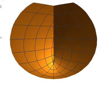
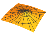
The following figures are examples of rotating GRT-surfaces for some \ell functions and constants aa and bb.

Refer to caption
Refer to caption
Figure 3: (t)=t2+t+1\ell(t)=t^{2}+t+1,  a=1,b=0a=1,\hskip 5.69046ptb=0
Refer to caption
Figure 4: (t)=t2+t+1\ell(t)=t^{2}+t+1,  a=0,b=1a=0,\hskip 5.69046ptb=1
Refer to caption
Refer to caption
Figure 5: (t)=cos(t)\ell(t)=\cos(t),  a=1,b=0a=1,\hskip 5.69046ptb=0
Refer to caption
Refer to caption
Figure 6: (t)=sinh(t)\ell(t)=\sinh(t),  a=1,b=0a=1,\hskip 5.69046ptb=0

Bibliografía

  • [1] A.V. Corro, D.G. Dias, Classes of generalized Weingarten surfaces in the Euclidean 3-space,Adv.Geom. 2016;16(1)45–55
  • [2] A. Martinez, P. Roitman, A class of surfaces related to a problem posed by Élie Cartan, Ann.Mat. Pura Appl,195,513–527
  • [3] W. Ferreira, P. Roitman, Area preserving transformations in twodimensional space forms and classical differential geometry, Israel J.Mat,190,325–348
  • [4] A.V. Corro, R. Pina, M. Souza, Classes of Weingarten surfaces in 𝕊2×\mathbb{S}^{2}\times\mathbb{R}, HOUSTON JOURNAL OF MATHEMATICS, v. 46, p. 651-664, 2020.
  • [5] P. Appell,, Surfaces telles que lórigine se projette sur chaque normale au milieu des centres de courbure principaux., Amer. J. Math. 10(1888),175–186. MR1505475 JFM 19.0825.01
  • [6] A.V. Corro, C.M. Riveros, D.G. Dias, A class of generalized special Weingarten surfaces, International Journal of Mathematics Vol. 30, No. 14 (2019) 1950075
  • [7] A.V. Corro, K. Tenenblat, Ribaucour transformations revisited., Comm. Anal. Geom. 12(2004), 1055–1082. MR2103311 (2005j:53063) Zbl 1090.53055
  • [8] A.V. Corro, M.J.C. Mendez, Ribaucour-type Surfaces, arXiv:2012.02132 [math.DG].
  • [9] G. Tzitzéica, Sur une nouvelle classe de surfaces., Rend. Circ. Mat. Palermo 25 (1908), 180–187. JFM 39.0685.05
  • [10] A.V. Corro, C.M. Riveros, K. Fernandes Ribaucour surfaces of harmonic type International Journal of Mathematics Vol. 33, No. 1 (2022) 2250006