Generalized quantum similarity learning
Abstract
The similarity between objects is significant in a broad range of areas. While it can be measured using off-the-shelf distance functions, they may fail to capture the inherent meaning of similarity, which tends to depend on the underlying data and task. Moreover, conventional distance functions limit the space of similarity measures to be symmetric and do not directly allow comparing objects from different spaces. We propose using quantum networks (GQSim) for learning task-dependent (a)symmetric similarity between data that need not have the same dimensionality. We analyze the properties of such similarity function analytically (for a simple case) and numerically (for a complex case) and show that these similarity measures can extract salient features of the data. We also demonstrate that the similarity measure derived using this technique is -good, resulting in theoretically guaranteed performance. Finally, we conclude by applying this technique for three relevant applications - Classification, Graph Completion, Generative modeling.
I Introduction
Notions of (dis)similarity are fundamental to learning. For example, they are implicit in probabilistic models that use dissimilarity computations to derive model parameters. In contrast, nearest neighbor (KNN) or Support Vector Machines (SVM) methods explicitly find training instances similar to the input. Notions of similarity also play a fundamental role in human learning. It is well known that people can perceive different degrees of similarity. The semantics of such judgments may depend on both the task at hand and the particulars of data. Since manually tuning such similarity functions can be difficult and tedious for real-world problems, the notion of automatically learning task/data-specific similarity () from labeled data have been introduced [1, 2, 3, 4, 5]. In general, these learning methods are based on the intuition that a good similarity function should assign a large/small score to a pair of points in the same/different classes.
The most common way to model similarity is to use a distance metric as a model for the desired similarity measure. By definition, obeys the properties , , , where with the data space. An important effect of this is the transitive nature of the similarity function i.e. derived from obeys the following, if and , then . The class of similarity maps attainable by these methods is just a subset of general similarity maps.
Another major technique used in classical machine learning is manifold-learning. This method aims to learn a low-dimensional structure in data under the assumption that the data lie on a (possibly non-linear) manifold. Examples of such methods include[6] local linear embedding[7], multidimensional scaling[8], Laplacian Eigenmaps[9] etc. These methods, by nature, produce only symmetric similarity measures i.e. .

Meanwhile, much work has been done to marry quantum computing and classical machine learning techniques to construct practical quantum algorithms compatible with the Noisy Intermediate-Scale Quantum (NISQ) era. One approach is to use parametrized quantum circuits (PQC) to define a hypothesized class of functions that potentially might offer access to a class of models beyond what is possible with classical models. Such quantum learning/variational algorithm have been used for various applications[10, 11, 12, 13, radha2021quantumwick]. Theoretical works have been successful in showing such quantum models exist for specific synthetic problems[14, 15, 16]. Specific classes of such quantum machine learning (QML) algorithms can be mathematically connected to their classical counterpart - kernel methods[17, 18]. In these methods, the learning is based on the kernels that are calculated between two given data points after mapping them to a latent space. This kernel can be made of PQCs, which, when trained, define distances on the latent space[19].
In this paper, we show that a general framework of such quantum embedding maps expands the class of algorithms from distance metric learning to (a)symmetric-similarity learning ones, which we call GQSim. This general class of QML algorithms has striking similarities with the classical similarity learning methods, including Siamese networks[20]. We show that these extensions allow for more general properties like intransitivity, asymmetry, etc., enabling us to learn a larger class of similarity maps than just distance-based similarity. Finally, one advantage of this technique is the ability to compare objects belonging to possibly different spaces, as shown schematically in Figure 1. Formally, given and data instances from two different sources/base space, and set of triplets where , the task is to predict for a pair of unseen instances with certain non trivial properties for (like asymmetry). Note that even though we have , the same technique can easily be extended to non-regression type problems by having . Such learning applications abound in nature; for instance, learning the sentence similarity between two different languages would generally be asymmetric and involve two different spaces.
We start by formulating the problem at hand and its underlying theory in section II. In section III, we first discuss analytically various details of the GQSim methods, including the effect of partial measurement. We illustrate this by solving a toy-problem analytically. Second, in subsection III.2 we pick a numerical problem of learning similarity between two different subspaces made up of synthetic images and points in to demonstrate the generalizability of the learned model. section IV discusses similarity learning in various applied settings, and finally, we summarize our findings in section V.
II Formalism
For sets and , assume we are given set of elements and the corresponding set of similarity measure where for all with . Our goal is to learn the model that is used to predict the similarity between unseen elements in . We first start by generalizing metric learning for multi-subspace setting after which we introduce the framework for learning asymmetric similarity. Even though , for the sake of discussion, we will restrict ourselves to being binary values of either similar or dissimilar. Learning of is done by using parameterized quantum circuits, details of which are discussed in subsubsection III.2.1.

II.1 Multi-subspace metric learning
Given with cardinality such that pairs are deemed related () and are unrelated (). Then we try to learn a distance function
such that
| (1) |
for some small constants . Here, need not satisfy the usual axioms of a distance metric, such as symmetry, which may not even make sense as the inputs come from different spaces. The problem can also be phrased in terms of a similarity measure , which simply reverses the inequalities: should be large when and are similar and small when they are dissimilar.
We consider of the form
| (2) |
where the feature maps , encode the raw input data in a common Hilbert space . Concretely, let be the Hilbert space of a quantum computer with qubits, and let be the space of complex-linear operators on equipped with the Hilbert-Schmidt inner product. Following [21], define the feature maps
| (3) | ||||
where , are parameterized quantum circuits. Then
| (4) |
where the similarity measure
| (5) | ||||
is nothing but the overlap between states and . There are multiple methods to efficiently compute Equation 5 using a quantum device. It can be measured experimentally by first preparing the state and then computing the probability that all qubits measure to as shown in Figure 2(b). Alternatively, one can prepare the states , in two separate -qubit registers and performing a SWAP test with an ancilla qubit. The latter scheme trades circuit depth for width.
II.2 Generalized similarity learning
In the previous scenario, we formulated the picture where data in each individual space is mapped by a unique embedding to a Hilbert space. The quantum feature maps are hitherto defined by applying unitaries to a standard -qubit state . We will explore two variations of Equation 5, which by slightly tweaking, generalizes the previous setting.
Consider first a simple variant of the SWAP test method. Recall that in this setup, the feature maps , act on separate registers of qubits each. For , perform the SWAP test only on the first qubits of each register to obtain
| (6) |
where the (mixed) states
| (7) | |||
| (8) |
are the partial trace of the original density matrices over the last qubits, such a circuit is shown in Figure 2(d). When , encodes classical data into an -qubit system by applying a possibly non-unitary CPTP map to the initial state .
The second tweak comes by slightly changing modifying how Equation 5 is measured without SWAP test. An alternative for calculating expectation value, as mentioned previously, is to apply to and measure the probability that all qubits return . Instead, we will now only inspect the first qubits to obtain another modified similarity
| (9) | ||||
| (10) |
where . This circuit is shown in Figure 2(c).
One way to think of this quantity is to regard the correspondence
as an embedding of pairs . One might more suggestively write for some effective as shown in Figure 3. Ideally, all similar pairs should align perfectly with and dissimilar pairs should be orthogonal to . Here, we do not lose generality by mapping it to as any other arbitrary state can be mapped back to by a unitary which then can be absorbed into the embedding parameterized unitary. Measuring only some of the qubits effectively takes a partial trace over the remaining ones. Note that unlike the previous formulation, is need not be symmetric in and , even when .

II.3 Goodness of similarity learning
It is crucial to understand what it means for a pairwise functional maps to be a “good similarity function” for a given learning problem.
Balcan et al. [22] proposed a new learning theory for similarity functions. This framework aims to generalize the learning techniques of kernels by relaxing some of the constraints we are currently interested in. They give intuitive and sufficient conditions for a similarity function to guarantee performance. Essentially, a similarity function () is -good if a proportion of examples are on average more similar to examples of the same class than to examples of the opposite class for a proportion of examples. This is explicitly proved for a general which need not be a metric that satisfies positive semi-definiteness or symmetry. Given a -good , it can be shown that can be used to build a linear separator in an explicit projection space that has a margin and error arbitrarily close to .
Definition II.1 (Balcan et al. [22])
A similarity function () is -good function for a learning problem if there exists a (random) indicator function defining a (probabilistic) set of points such that the following conditions hold:
-
1.
A probability mass of examples satisfy
-
2.
.
Formally defined in Definition II.1, it can also be shown that the set of similarity maps defined by this is strictly larger than the set of metric maps and also includes non-positive semi-definite kernels and asymmetric maps. With the above definition, Ref[22] proved the following theorem
Theorem II.1 (Balcan et al. [22])
Let be a -good similarity function for a learning problem for a learning problem . Let be a (potentially unlabeled) sample of landmarks drawn from . Consider the mapping defined as following
Then, with probability over the random sample the induced distribution in has a separator error at most relative to margin at least .
Theorem II.1 states that, if enough data is available for the problem , then for a -good similarity function, with high probability there exists a low-error (arbitrarily close to ) linear separator in mapped -space. This framework of -good functions opens the door for us to evaluate the performance that one can expect a global linear separator to have, depending on how well a similarity function satisfies Definition II.1. We will see in subsection III.2 that this method, at least numerically, can separate the classes as needed by definition.
III Discussion
We will start with a qualitative discussion on similarity learning methods introduced in subsection II.1, following which we solve a toy embedding explicitly to understand the intricacies of these methods. Next, we explore a more complex example of learning the similarity between a synthetic image set and abstract 2D space, and numerically show that this learning method can learn salient encoded features of the images.
III.1 Analytical Discussion
By taking in metric learning setting, we reduce to the framework of classical metric learning where the sought-after is assumed to be a distance (pseudo-)metric in the usual sense. Thus, should satisfy the following properties with equality when ; , and for all triples . One way to enforce these constraints is to seek a distance function of the form
where is some neural network mapping into some latent Euclidean space . This construction, depicted in Figure 4, is called a Siamese neural network [20]. By taking as a quantum feature map as in the previous subsection, we have
| (11) |
where is a parameterized quantum kernel[23, 24]. As noted in Ref.[24, Appendix A], the training criterion Equation 1 implicitly guides the latent space embeddings to separate dissimilar pairs while compressing similar pairs together.

Next, in case of the similarity , as hinted in subsection II.2, when , is a non-unitary CPTP map. This thus enriches the family of feature maps at our disposal compared to the previous case. Intuitively this can be understood as following, we prepare two quantum states that map classical data and to their respective states . In the previous multi-space metric learning case, we required that (dis)similar elements be mapped (far)close to each other in the Hilbert space with dimension . In contrast, similarity defined in Equation 6 requires that dis)similar gets mapped (far)close to each other in the Hilbert space . This is similar to the projective SWAP test used in Ref[25].
We will now offer some heuristics for the more general similarity measure . It is easier to cluster points together in lower-dimensional spaces, which may help when similar raw data are far apart in their ”native” spaces . The trade-off is that separating points becomes hard. The number of qubits measured changes the relative difficulties of satisfying the training constraints.
Precisely, suppose one measures of the qubits. Then if , the possible embeddings that satisfy the constraint live in a subspace of dimension . This space is spanned by all basis states . On the other hand, if , the states that satisfy constitute a subspace of dimension . The ratio describes the relative difficulties of the training constraints. In the scenario where , we have , i.e we provide equal volumetric space in the model to place similar and dissimilar data points. In contrast, when , where we provide larger space for dissimilar points to live. This gives us the ability to tune the model space we are working with based on the data provided, for instance for an highly imbalanced data set (when ), one can choose based on if .

We illustrate these considerations with a toy example. Consider the following simple two-qubit circuit – where and are the Pauli and rotations by angle on qubit – and the state . can be interpreted as a embedding of in a Hilbert space for a particular choice of parameters. By traversing , we can trivially look at the entire embedding space accessible by the constant ansatz . We can thus look at the number of pairs of similar and dissimilar points that are accommodated by this ansatz based on the measure for various (in this case ), both of which is shown in Figure 5(a) as circuits. As shown in appendix A one gets
| (12) | ||||
| (13) |
In Figure 5(a), we plot and for all values of . Intuitively, ’s closeness to a value of () indicates the paired points are (dis)similar to each other. We see that in the case of we have exactly 4 points in the space that are maximally similar to each other. In contrast, a huge set of points with an almost flat region have a similarity measure of . Comparatively, in , we have lifted a majority of this flat region to support more points that are similar to each other. To better understand this, we also look at the Density of States (DoS) of for both the cases. The following defines this,
| (14) |
essentially counts the number of points inside each fundamental unit of similarity. Figure 5(b) shows the DOS, where we see a peak close to , for indicating that this measure allows for a high imbalance between similar and dissimilar points. In the case of , as discussed previously, we have a perfectly even split of volume between similar and dissimilar points with mid (dis)similarity measure being .
Let us now place the above problem in the setting of retrieval problem to gauge the ability of the respective family of similarity measures. Given two subspaces , and , we strive to find some point that is most similar to but most dissimilar to . This problem can be formulated as minimizing
| (15) |
where
| (16) |
for some similarity measure and loss function . measures the loss of how well the similarity measure has performed. As a first illustration, we pick and and then calculate using the same embedding . This is shown in Figure 6(a), where the dotted lines use the measure while the red line uses . Since the quantum embedding map is the same for both the cases, they both have the same optimal . We see that the loss function, which can be used as a surrogate to quantify how good the similarity measure is in separating the optimal , is much lower/deeper in the case of . Thus partial measurement of is able to attain a better separation than . To complete the analysis, we calculate the quantity
| (17) |
where is the optimal for the pair . quantifies the (dis)advantage one gets by using instead of . Figure 6(b) plots , where one sees that at worst case, we do not get any larger separation/better performance using partial measurement. But there are cases (as seen in Figure 6(a) and indicated by non zero value in (b)), where the (dis)similarity of is better in partial measurement.

III.2 Numerical Discussion
III.2.1 Experimental setup
Unless otherwise stated, the following setup is adopted throughout the numerical experiments. We use the QAOA embedding[19], which typically first encodes each input feature in the angle of a separate gate, then creates entanglement using a combination of parameterized one-qubit and two-qubit rotation. We use layers of size and qubits count of . We use the same basic ansatz to embed both features but allow the underlying parameters to vary independently for each feature; in other words, in (3) we take . Our training data comes in the form of subsets of similar and dissimilar pairs, respectively. By construction, our similarity function takes values in the interval . We wish to find parameters such that ideally satisfies on and on . We seek to minimize the cost function
| (18) |
where
Whereas most machine learning literature searches for the optimal parameters using some form of stochastic gradient descent, we employ the COBYLA optimizer [26]. This is a gradient-free method designed for noisy cost landscapes. Since it is expensive to evaluate the loss Equation 18 over the entire dataset, whenever it is required to evaluate the loss, we approximate it by a sum over a randomly chosen subset of the terms, normalized by the batch size of , justification for this choice is given in Appendix B.
III.2.2 Experiment/Discussion
Image data
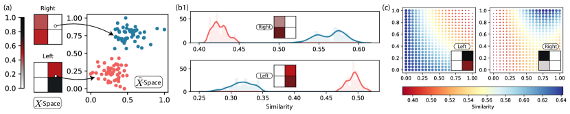
: To better understand the capabilities of these learning models, we here show a full working flow of the algorithm. We synthetically generate images as shown in Figure 7(a) where the pixel values of images are filled from a uniform random distribution between . We split the image data into two sets where we reset the right half of the pixels to for one set and the left half to in the other set. We label these two subsets as “right” and “left”. This now forms the space of our data. For -space, we generate points clustered into 2 sections (shown as red and blue in (a)) in . For the training data, we consider “left”(“right”) images in to be similar to red(blue) points in . Using this, we then generate our training points made up of for all points and with being () for (dis)similar pairs. We then start the learning process to find the optimal parameters () that minimize the loss given in Equation 18. We use as the similarity model.
Performance
: Once we have the optimal angles, there are multiple ways to test the performance of this model. First, we generate a new random “left” () and “right” () image and calculate the following four quantities - , , , where is the red/blue point in -space that was used for training. We plot the histogram/density of these points in Figure 7(b), where we plot the similarity value of test image shown in inset with red points (shown as red line) and blue points (shown as blue line) for (b1) and (b2) . We see that in both cases, the network successfully separates the similarity values of how close the left/right image is to the blue/red points depicted by the peaks in each distribution. Second, we see that is closer (higher similarity value) to blue points than to red points while the case is reversed for the left value. This is consistent with how we expect the model to behave. This shows that the model has not only trivially learned what it means to be left image and what it means to be the right image, but how this feature associates to a different subspace - . This brings us to the discussion in subsection II.3, where we introduced the concepts of -good similarity function. The figure shows that the average distance between samples in classes is well separated for their corresponding classes in space. Numerically we verified that this is not just true for a subset of points in , but for all points in .
Another gauge of the model performance is to look at where in the -space does our model place a given point in -space. To this end, we chose another random and calculated its similarity on a uniform grid space in . This is shown in Figure 7(c), where the color and size of each grid point corresponds to the learned similarity measure of the image in the inset. We see that the most similar points in for the left image (indicated by blue color) are around the lower left, while for the right, it is around the upper right corner. This is indicative of the initial mapping we learned from where the points in space form clusters in the left bottom, and top right parts of the space.
Generalizability of model
: To answer the question about the generalizability of the learned model, we now generate out-of-sample images given by the following pixel value
| (19) |
where is a random variable generated from a truncated normal distribution with mean and variance , where is a relatively small number (in our case we choose . Thus we have the two extremes , where belongs to left(right) image groups while it interpolates between left and right as a function of . This is shown in Figure 8(top).

We can quantify the network’s performance in this scenario by looking at the maximal separation between the similarity of from the training data’s red and blue points. We do this by calculating the Wasserstein distance () between the distributions formed by these similarities. For example, in Figure 7(b1), we calculate the Wasserstein distance between the red and blue distributions. We do this for different randomly generated images for each . Figure 8(bottom) shows the result of such calculation with error bars indicating the variance of the runs. Intuitively measures the (in)distinguishably of in space. Since in our mapping, left and right images are separable in space, we expect to see a high distance value at these extremes. As we approach , the image becomes equally (dis)similar to both red and blue points in and hence the distance between the respective similarity distributions attain . This is shown in Figure 8(bottom). This is phonologically similar to the ordered to disordered phase transition detected using classical neural network in Ref[27]. Thus by just training the model with the extremities (), the network has learned to detect higher-order features enabling us to detect unseen transitions. It shows that the final achieved similarity scores are discriminative not just because of local information about the images, rather a combination of both local and global properties.
IV Applications
Although similarity measures can be used for a wide range of applications, we choose three such applications to analyze and understand the technique. First, we show the trivial example of how similarity learning can be used for classification. Then, we illustrate a practical example of graph link completion problem using similarity learning. Finally, we show that ability to differentiate parameters in quantum circuits efficiently gives us the ability to use the learned model as a generative model.
IV.1 Classification
Classification tasks and the notion of similarity are deeply connected. Suppose we are given clusters of data
To classify a new data point , we want to determine the class “most similar” to - in other words, a fidelity classifier[23, Appendix C]. Here, maximizing the separation of embedded data from different classes amounts to minimizing the empirical risk of the classifier for a linear loss function. An alternative method, which we do not pursue here, is to use the trained kernel in a support vector machine classifier as proposed by Hubregtsen et al [24]. Instead, it suffices to compare with a representative sample from each class. While the usual distance in provides a naive notion of similarity, distance measures tailored to the data may perform better if the classes are irregularly shaped. In Figure 9, we show our GQSim being used for where (a) is multi-class classification and (b) is a more complex structure for similarity measure. In (a), we compare each point in the the space to single sample from each train class to do a one shot classification while in (b) we compute the similarity and normalize it to 1 for each point in space to get the probability of them being similar to yellow or purple family.

The image example discussed in subsection III.2 is a toy model of the following classical problem: given clusters of images and crude information about the clusters, one can use this information to encode the images in a different subspace . This information is termed side information, and it appears naturally in many applications. For example, when classifying images containing {house, dog, cat}, we know that even though they belong in discrete categories, the distance between categories dog-cat is closer than dog/cat-house. Another example of side information is categorizing the rating of a given movie in {1,2,3}. Even though each movie has a category, one has the information that the categories are ordered i.e . This information can be encoded in space by manually choosing clusters for , say in , such that center of . Thus, now learning the similarity between the movie space and space and using this similarity to categorize movies has more implied structure built into it than directly classifying them.
IV.2 Graph Completion
Link prediction[4] is an important aspect of network analysis and an area of key research. Graph completion problem[28] is a subset of link prediction, where it is assumed that only a small sample of a large network (e.g., a complete or partially observed sub-graph of a social graph) is observed, and one would like to infer the unobserved part of the network. To formalize the setting, we assume there is a true uni directed unweighted graph on distinguishable nodes with its own attributes for with an adjacency matrix where denotes an absent edge and denotes a connected edge. We then assume that only a partially observed adjacency sub-matrix with induced by a sample sub-graph with , of original graph is given. We are now interested in predicting the complete adjacency matrix based on the partially observed sub-matrix using the learned similarity measures of the node attributes . For example, in a social community network, the nodes might represent the individuals, and the link of nodes represents the relations between the individuals. The attributes for each node could include the person’s metadata like interest, age, location, occupation, etc. The more similar attributes of the two nodes are, the higher probability they have a relationship and are linked in the network.

As an example, in Figure 10 we will associate attributes of each node with a dimensional data coming from unique distributions . Edges are then connected () to nodes having attributes from the same distribution and not connected if their attributes correspond to a different distribution. This defines the real hidden graph . After this, we randomly select of the edges to create the sub-graph . This is then fed into the algorithm to learn the similarity between the nodes, which is then used to complete the graph. Since we have chosen an uni-directed graph , connection between is going to be the same between . This symmetry is forced in the model by setting of the learning model, i.e. we choose to embed both comparing points with the same embedding. Clearly, for general directed multigraph, one needs to go beyond symmetry and have the property that . Moreover, in the case of a directed multigraph, one needs to allow for nontrivial to indicate loops in the graph potentially. For these cases, one may opt to use the generalized similarity learner to embed the points in different embedding and trace out parts of the Hilbert space.
The figure shows the graph nodes being plotted in a 2D space, with each node placed corresponding to its attribute. Red lines indicate the connected nodes, while dotted lines indicate no connection. Missing lines in the left figure correspond to the lack of information. The right figure shows the predicted complete matrix. As seen from the figure, the points from the same spatial cluster are connected while the nodes with attributes belonging to different are disconnected. In the experiments where we have as Gaussian with random spread , a reduced graph with edges as little as reproduces the final graph with accuracy.
IV.3 Generative model

Given a learned similarity measure between two different spaces, one can now use support points to generate new data in the other space. More concretely, given a learned similarity measure , and a support point , one can generate an unseen data point in using the following optimization problem
| (20) |
Such tasks occur naturally in many scenarios; for example, in the case of language translation between two languages, one can generate new unseen similar sentences in another language based on learned similarity measure. Despite being an optimization problem in feature space, this is efficient in our quantum case. This is because features are directly encoded as parameters in our PQCs and thus can be efficiently differentiated[29]. To illustrate this, we again invoke the example discussed in subsection III.2. Given an image, we solve Equation 20 to find the closest point in for a given image of type “right”. We show this in Figure 11, where we plot the cost function of this minimization problem and the minimization steps.
V Summary
We have considered a generalization of similarity learning techniques in the quantum setting. PQCs express similarity functions with a richer set of properties like (a)symmetry, intransitivity, and even multi-space metrics. Similarity learning boils down to learning pair wise similarity by embedding the input features in Hilbert space. We illustrate the effect of using partial measurements and their use in modeling imbalanced data. Using a synthetic image data set with left and right pixels blocked, we learn the similarity of these images arbitrary points in space. This example is also used to illustrate the generalizing capability of these learned models. We use the model to detect phase transition from left-like image to right-like image. Finally, we show three applied use cases where learned similarity can be used. Classification, being a trivial use case of learning similarity, can be augmented to encode given side-information about the data using the multi-space property of generalized similarity learning. Graph link completion problem can be rephrased as a similarity learning problem, which we numerically showed for a simple example. Finally, we demonstrate how similarity models can be used as generative models to generate unseen data in the complementary space, given corresponding data in the original space. Nevertheless, there are still critical challenges regarding the choice of the PQC embedding one chooses for the given data.

V.1 Acknowledgments
The authors thank Jack Baker for insightful discussions.
Appendix A Analytical details of toy-problem
We here outline the details of setup discussed in subsection III.1. As discussed, one can think of the PQC in Figure 5 (a1/a2) in two equivalent ways - 1. (or move the to ) or 2. . First one corresponds to individual mappings while the second one takes the pair values and map it to a point in Hilbert space, both of which are equivalent views. The matrix form of is given by
| (21) |
from which we see that
| (22) |
which is given in Equation 12. Similarly, we get Equation 13 by computing
| (23) |
which trivially from Equation 21.

Appendix B Optimization for learning
Throughout the paper, as mentioned in subsubsection III.2.1, we have used the COBYLA[26] optimization scheme for learning the similarity. Because of the costly function evaluations required to compute pair-wise terms in Equation 18, we apply the heuristics of stochastic batching to reduce the number of evaluations. The heuristics are as follows:
-
•
We pick random pairs of points from each similar/dissimilar pairs from the training set for iteration making the set .
-
•
We compute
-
•
We use this in the COBYLA optimization routine until convergence is achieved.
We caution that this “stochastic” form of COBYLA is similar to stochastic gradient descent techniques[30], but has no theoretical backing yet in the literature. Having said that, this heuristic, although employed for reducing the computational time, could offer potential benefits that exist in stochastic gradient descent. Primarily, the stochastic batching heuristic could be used to reduce the number of function evaluations required for learning and push towards the global minimum much faster than non-stochastic, where we have lots of local maxima/minima. One can think of this as approximating the ”effective” manifold of the cost function having an error bar. To this end, it is essential to understand what numerical choice of is best. Naively one could assume that is indeed data-dependent as the features in the data could make the landscape more complicated. To understand this better, we calculate the effect of on the cost function by computing the average of over a range of values for various runs. We then plot the average cost function over the range of for two different similarity learning problems - Classifying two clustered blob data set and two moon data set, which is shown in the Figure 12.
We see that, at least in the case of blob vs. moon, where one would assume learning blob is more straightforward than learning similarity between moon, the batch size dependence on the variance of cost manifold is almost the same. We also observe that around batch size , the variance in cost manifold for both blob and moon data set. This is because the cost function is very smooth, and the batch size is big enough to approximate the exact cost manifold, despite the actual batch size cost manifold having pairs. We thus use a batch size of throughout the numerical experiments in the paper.
Appendix C The effect of partial measurements

We present some preliminary data on the effect of measuring only some qubits in the image data experiment of subsubsection III.2.1. For each , generate two separated clusters, labeled “red” and “blue”, of points in the -dimensional unit cube ; the preceding discussion considered the case . As before we try to learn the associations (“Right”, {blue cluster}), (“Right”, not {red cluster}), (“Left”, {red cluster}), (“Left”, not {blue cluster}). We then run instances of randomly generated synthetic data of this form and run the learning algorithm for all the allowed trace qubit dimension. Figure 13 shows the loss as a function of training iterations for each dimension of .
Next we run the training multiple times for each dimension of and for each choice of qubits to be measured. The average (mean) minimum training losses encountered during each training is shown in Figure 14, together with their variance. Overall there appears to be a slight degradation in training quality as more qubits are measured. Note that for a given problem (denoted by color in plot ), all the trace experiments are done with the same data-set. We see that smaller Hilbert space seem to attain lower average cost value compared to measuring all qubits. We see that the variance in the cost drastically decreases as well. Both these phenomenon point us in future directions to explore for further understanding the effects of partial measurements in learning models.
References
- Schultz and Joachims [2004] M. Schultz and T. Joachims, Learning a distance metric from relative comparisons, Advances in neural information processing systems 16, 41 (2004).
- Shalev-Shwartz et al. [2004] S. Shalev-Shwartz, Y. Singer, and A. Y. Ng, Online and batch learning of pseudo-metrics, in Proceedings of the twenty-first international conference on Machine learning (2004) p. 94.
- Chechik et al. [2009] G. Chechik, V. Sharma, U. Shalit, and S. Bengio, An online algorithm for large scale image similarity learning, (2009).
- Bellet et al. [2013] A. Bellet, A. Habrard, and M. Sebban, A survey on metric learning for feature vectors and structured data, arXiv preprint arXiv:1306.6709 (2013).
- Nicolae et al. [2015] M.-I. Nicolae, É. Gaussier, A. Habrard, and M. Sebban, Joint semi-supervised similarity learning for linear classification, in Joint European Conference on Machine Learning and Knowledge Discovery in Databases (Springer, 2015) pp. 594–609.
- Bengio et al. [2003] Y. Bengio, J.-f. Paiement, P. Vincent, O. Delalleau, N. Roux, and M. Ouimet, Out-of-sample extensions for lle, isomap, mds, eigenmaps, and spectral clustering, Advances in neural information processing systems 16, 177 (2003).
- Roweis and Saul [2000] S. T. Roweis and L. K. Saul, Nonlinear dimensionality reduction by locally linear embedding, science 290, 2323 (2000).
- Cox and Cox [2008] M. A. Cox and T. F. Cox, Multidimensional scaling, in Handbook of data visualization (Springer, 2008) pp. 315–347.
- Belkin and Niyogi [2003] M. Belkin and P. Niyogi, Laplacian eigenmaps for dimensionality reduction and data representation, Neural computation 15, 1373 (2003).
- Kerenidis et al. [2019] I. Kerenidis, J. Landman, and A. Prakash, Quantum algorithms for deep convolutional neural networks (2019), arXiv:1911.01117 [quant-ph] .
- Dallaire-Demers and Killoran [2018] P.-L. Dallaire-Demers and N. Killoran, Quantum generative adversarial networks, Physical Review A 98, 012324 (2018).
- Radha [2021] S. K. Radha, Quantum constraint learning for quantum approximate optimization algorithm (2021), arXiv:2105.06770 [quant-ph] .
- Coyle et al. [2021] B. Coyle, M. Henderson, J. C. J. Le, N. Kumar, M. Paini, and E. Kashefi, Quantum versus classical generative modelling in finance, Quantum Science and Technology 6, 024013 (2021).
- Liu et al. [2021] Y. Liu, S. Arunachalam, and K. Temme, A rigorous and robust quantum speed-up in supervised machine learning, Nature Physics 17, 1013 (2021).
- Sweke et al. [2021] R. Sweke, J.-P. Seifert, D. Hangleiter, and J. Eisert, On the quantum versus classical learnability of discrete distributions, Quantum 5, 417 (2021).
- Huang et al. [2021] H.-Y. Huang, M. Broughton, M. Mohseni, R. Babbush, S. Boixo, H. Neven, and J. R. McClean, Power of data in quantum machine learning, Nature communications 12, 1 (2021).
- Schuld [2021] M. Schuld, Quantum machine learning models are kernel methods, arXiv e-prints , arXiv (2021).
- Pronobis and Müller [2020] W. Pronobis and K.-R. Müller, Kernel methods for quantum chemistry, in Machine Learning Meets Quantum Physics (Springer, 2020) pp. 25–36.
- Lloyd et al. [2020a] S. Lloyd, M. Schuld, A. Ijaz, J. Izaac, and N. Killoran, Quantum embeddings for machine learning (2020a), arXiv:2001.03622 [quant-ph] .
- Bromley et al. [1993] J. Bromley, J. W. Bentz, L. Bottou, I. Guyon, Y. LeCun, C. Moore, E. Säckinger, and R. Shah, Signature verification using a “siamese” time delay neural network, International Journal of Pattern Recognition and Artificial Intelligence 7, 669 (1993).
- Havlíček et al. [2019] V. Havlíček, A. D. Córcoles, K. Temme, A. W. Harrow, A. Kandala, J. M. Chow, and J. M. Gambetta, Supervised learning with quantum-enhanced feature spaces, Nature 567, 209 (2019).
- Balcan et al. [2008] M.-F. Balcan, A. Blum, and N. Srebro, Improved guarantees for learning via similarity functions, (2008).
- Lloyd et al. [2020b] S. Lloyd, M. Schuld, A. Ijaz, J. Izaac, and N. Killoran, Quantum embeddings for machine learning, (2020b), arXiv:2001.03622 [quant-ph] .
- Hubregtsen et al. [2021] T. Hubregtsen, D. Wierichs, E. Gil-Fuster, P.-J. H. S. Derks, P. K. Faehrmann, and J. J. Meyer, Training quantum embedding kernels on near-term quantum computers, (2021), arXiv:2105.02276 [quant-ph] .
- Lloyd et al. [2013] S. Lloyd, M. Mohseni, and P. Rebentrost, Quantum algorithms for supervised and unsupervised machine learning (2013), arXiv:1307.0411 [quant-ph] .
- Powell [2007] M. J. Powell, A view of algorithms for optimization without derivatives, Mathematics Today-Bulletin of the Institute of Mathematics and its Applications 43, 170 (2007).
- Shiina et al. [2020] K. Shiina, H. Mori, Y. Okabe, and H. K. Lee, Machine-learning studies on spin models, Scientific reports 10, 1 (2020).
- Bai et al. [2019] L. Bai, L. Rossi, L. Cui, J. Cheng, and E. R. Hancock, A quantum-inspired similarity measure for the analysis of complete weighted graphs, IEEE transactions on cybernetics 50, 1264 (2019).
- Benedetti et al. [2019] M. Benedetti, E. Lloyd, S. Sack, and M. Fiorentini, Parameterized quantum circuits as machine learning models, Quantum Science and Technology 4, 043001 (2019).
- Bottou [2010] L. Bottou, Large-scale machine learning with stochastic gradient descent, in Proceedings of COMPSTAT’2010 (Springer, 2010) pp. 177–186.