Generalized Nonlinear and Finsler Geometry for Robotics
Abstract
Robotics research has found numerous important applications of Riemannian geometry. Despite that, the concept remain challenging to many roboticists because the background material is complex and strikingly foreign. Beyond Riemannian geometry, there are many natural generalizations in the mathematical literature—areas such as Finsler geometry and spray geometry—but those generalizations are largely inaccessible, and as a result there remain few applications within robotics. This paper presents a re-derivation of spray and Finsler geometries we found critical for the development of our recent work on a powerful behavioral design tool we call geometric fabrics. These derivations build from basic tools in advanced calculus and the calculus of variations making them more accessible to a robotics audience than standard presentations. We focus on the pragmatic and calculable results, avoiding the use of tensor notation to appeal to a broader audience, emphasizing geometric path consistency over ideas around connections and curvature. We hope that these derivations will contribute to an increased understanding of generalized nonlinear, and even classical Riemannian, geometry within the robotics community and inspire future research into new applications.
I Introduction
Nonlinear geometry is in many ways fundamental to robotics. Robotic configuration spaces are naturally modeled as manifolds [1], the classical mechanical dynamics of the robot is intimately linked to a Riemannian geometry [2], Gauss-Newton optimization has strong application in vision [3] and motion optimization [4] and those algorithms are closely related to Riemannian geometry [5, 6] natural gradients [7] which are core to many modern machine learning methods [8]. Despite their importance, however, even classical Riemannian geometry remains inaccessible to many roboticists. And beyond that, Finsler [9] and spray geometry [10], natural generalizations of Riemannian, are largely unheard of within the community. How many applications are out-of-reach as a result?
Our own work on Riemannian Motion Policies (RMPs) [11, 12] has led us to a study of what we call geometric fabrics [13, 14] as a formal provably stable model of reactive behavior, and to get there, we had to address this gap. Both Finsler and spray geometries proved critical for the development of that work, but were largely confined within opaque mathematical manuscripts mired with abstract concepts and foreign notation. The importance of the material, however, led us to entirely re-derive the foundations, rigorously, but in a language we could understand. This paper presents these re-derivations in a hope that they will be more accessible to a broader robotics audience and inspire new future applications.
We use notations of advanced calculus [15] as much as possible and build on the Calculus of Variations [16] (Finsler geometry maybe viewed as the geometry of these functional optima), and we draw connections to classical mechanics [17], Riemannian geometry [18, 2], and the interrelations observed in geometric mechanics [2]. We limit ourselves to a study of geometric path consistency which we call generalized nonlinear geometry (see Section II),111Our terminology differs from the literature. Equations exhibiting geometric path consistency are commonly called sprays in mathematics [10], and literature further develops more general geometry with a very similar name (a semi-spray), which doesn’t exhibit such path consistency. We, therefore, restrict the term geometry to imply this concrete notion of path consistency to aid intuition and reserve the term semi-spray in our applications [13] for these more general non-path-consistent equations. and show that Finsler geometries are a type of generalized nonlinear geometry (see Section III), inheriting their geometric consistency.

Manifolds [19] are a standard mathematical foundation of modern nonlinear geometry. However, these concepts can be very abstract and daunting for those unfamiliar. We, therefore, present our derivations in specific coordinates, following the conventions of many texts on classical mechanics [17]. For those familiar with the concepts, we can say we do so without loss of generality—the Euler-Lagrange equation is naturally covariant, enabling curvilinear changes of coordinates as necessary while traversing a manifold with no change to the underlying behavior; covariant behavior of more general nonlinear geometries can be expressed through a transform tree as was done in [12] in the definition of structured Geometric Dynamical Systems (GDS).
II Generalized nonlinear geometries
A generalized nonlinear geometry (known as a spray in mathematics [10]) is a second-order differential equation describing a smooth collection of paths. These paths are equivalence classes of trajectories all passing through the same points but differing in speed profile. In essence, we allow a trajectory to speed up or slow down arbitrarily, and as long as its geometric shape remains consistent (i.e. it passes through the same one-dimensional set (submanifold) of points in space) we say the trajectory follows the same path (i.e. is part of the equivalence class). Colloquially, similar to how we can think of an arbitrary second-order differential equation as a collection of trajectories (its integral curves), we can think of the geometry as a collection of tubes. Each tube represents a path and contains multiple trajectories (infinitely many of them), the collection of all trajectories following that path with differing speed profiles (see Figure 1).
Concretely, two trajectories are said to be equivalent, and hence along the same path, if they are a time reparameterization away from one another. Given a trajectory with time index denoted , a time reparameterization is a smooth, strictly monotonically increasing, nonlinear function denoted giving rise to a new time index . The time reparameterization creates a new trajectory . Since, for a given and corresponding , the points of the trajectories align
| (1) |
and since this relationship is a bijection (due to the strict monotonicity),222Formally, it is a diffeomorphism between coordinate charts of the same one-dimensional manifold of points. the two trajectories and pass through the same set of points and we say they follow the same path. Since and , we see velocities and accelerations under the time reparameterization are linked to one another as
| (2) | ||||
where notationally the dots are understood to be time derivatives w.r.t. their respective time indices. E.g. , and so forth. A smooth nonlinear geometry is defined by the collection of all time-reparameterization invariant smooth paths in a space. For every point and speed-independent direction vector , the nonlinear geometry defines a unique path eminating from that point following the specified initial direction .
Denoting the orthogonal projector projecting orthogonally to velocity as , the family of geometries we consider here are those characterized by a second-order differential equation of the form
| (3) |
where is a smooth function that is positively homogeneous of degree 2 (HD2) in velocities.333Generally, a function is said to be positively homogeneous of degree (abbreviated HD) if for [20]. Homogeneity of degree 1 and 2 is used in the definitions below as well. In this case, must be HD2, meaning for . We call equations of this form geometric equations.
Since the projector is reduced rank, there is solution redundancy. We will see that this redundancy precisely describes the ability to arbitrarily speed up or slow down along a trajectory while sticking to the same path.
The interior equation in isolation
| (4) |
we call the generating equation and is said to generate the geometry via its system of trajectories. Note that since has null space spanned by , solutions to the geometric equation are solutions to
| (5) |
where is a smooth function defining an acceleration along the direction of motion. We call this equation the explicit form geometric equation.
Theorem II.1.
All time reparameterizations of generating solutions are geometric solutions, and each geometric solution characterized by starting position and direction is a time reparameterization away from any generating solution with initial conditions for some .
Proof.
We first address reparameterization of generating solutions. Let be a generating solution trajectory and let be an arbitrary time reparameterization. In terms of its inverse (which always exists since is strictly monotonically increasing by definition), by Equations 2 we have
| (6) | |||
| (7) | |||
| (8) | |||
| (9) |
where . Thus, solves an explicit form geometric equation and is, therefore, a geometric solution.
Next, let be any solution to the geometric equation. Then at every point,
| (10) |
for some smooth function across the trajectory. Under a time reparameterization we get the following equation in terms of
| (11) | |||
| (12) | |||
Since is an ordinary second-order differential equation it has a unique solution for every initial condition . Under any of those solutions, the second term vanishes and we have (since ). Therefore, under such a time reparameterization, is a generating solution.
Moreover, since the initial condition defines the initial velocity which uniquely defines the generating solution moving in direction . Since any initial speed can be generated this way, every time reparameterization of this sort maps to a corresponding generating solution by initial conditions and every generating solution can be created by such a time reparameterization. Therefore, there is a bijection between time reparameterizations solving and generating solutions with initial conditions . ∎
The proof of the above theorem shows that any time reparameterization solving
| (13) |
induces a generating solution. Since solutions to Equation 13 are defined by their initial conditions, given a geometric solution , we can choose a time reparameterization (the inverse of ) so that is a generating solution whose velocity matches the geometric solution’s velocity at a given time (choose solving Equation 13 using initial conditions and ). That mapping from to instantaneous velocity-matching generating solution is smooth, so we can view the geometric solution as smoothly moving between generating solutions, using the redundant accelerations to do so by speeding up and slowing down along the direction of motion.
To illustrate path consistency, we designed a geometry, , that naturally produces particle paths that avoid a circular object in coordinates, , as
| (14) |
where is a differentiable map that captures the distance to a circular object and is a scaling gain. More specifically, , where and are the circle’s center and radius, respectively. Furthermore, is a barrier potential function, , where is a scaling gain. Altogether, produces an increasing repulsive force as distance to the object decreases, and makes homogeneous of degree 2 in . For this experiment, , for two scenarios: 1) , and 2) for the initial conditions, . Eleven vertically spaced particles that follow the above geometry are initialized with the two different initial speeds. Traced paths at the two different speeds are overlaid as shown in Fig. 1. Noticeably, the paths generated are completely overlapping confirming path consistency.
III Finsler geometry
Here, we derive a broad class of nonlinear geometries, known as Finsler geometries [9]. These geometries arise from Calculus of Variations problems [16] that generalize the notion of arc length to cases where length elements can vary by direction (Minkowski norms [something]). This section builds to a fundamental result showing that applying the Euler-Lagrange equation to these generalized length elements produces a Geometric equation (a Finsler geometry of paths) whose corresponding generator can be derived by applying the Euler-Lagrange equation to the length element’s energy form. Solutions to the latter conserve the derived energy and can thus be viewed as energy levels. And from the above analysis, we can characterize geometric solutions to Finsler geometries as smoothly transitioning between these concretely defined energy levels (generating solutions) by speeding up and slowing down along the direction of motion while remaining along the same common path.
III-A The Euler-Lagrange equation: a review
For completeness we review some background on the Calculus of Variations [16]. The Calculus of Variations studies extremal trajectory problems. Given a function of position and velocity, known as a Lagrangian, and the class of smooth trajectories ranging between two end points and , we can ask which of those trajectories minimizes the “total Lagrangian” across the trajectory:
| (15) |
where is understood to vary per trajectory based on its natural time interval. The integral is known as the Lagrangian’s action functional.
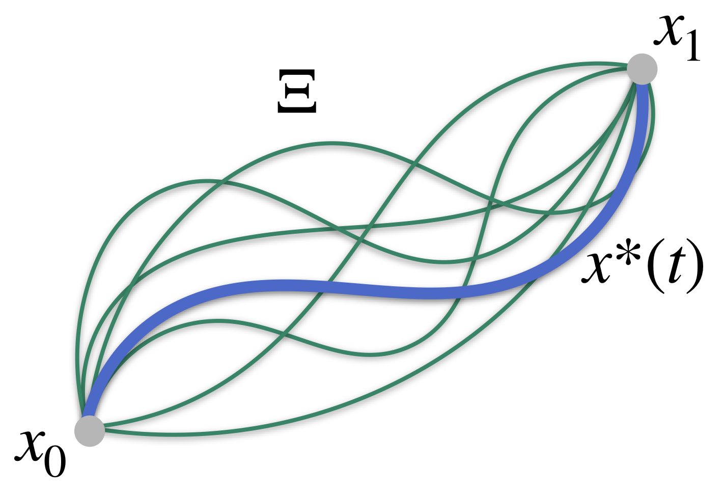
Figure 2 depicts this problem pictorally. Here the dark trajectories are possible candidates in and the dotted trajectory is the extremum.
We won’t derive it here, but extremal solutions are characterized by solutions to the following boundary-valued second-order differential equation:
| (18) |
This equation is important in its own right and is known as the Euler-Lagrange equation.444We write it in negated form here relative to the common expression from the Calculus of Variations [16] to match better with the equations of motion below, as we’ll see. By the theory of ordinary differential equations [19], this equation has unique initial-value solutions when it is point-wise well-formed for . (We’ll see that this means its velocity Hessian is invertible for . This won’t be the case for Finsler structures (and we’ll get the solution redundancy characteristic of geometric equations from that), but it will be the case for the corresponding energy-form generating equation.) This uniqueness of solution means that for any , we can play forward the Euler-Lagrange equation uniquely to generate a solution trajectory starting from that position and velocity. We can connect this solution back to the extremal problem by noting that every point encountered along this initial-value solution is a possible end point, and the solution to the initial-valued problem solves the boundary value problem with boundary constraints and . In other words, every subtrajectory of the initial-value solution is an extremal solution between its end points. Importantly, this enables us to consider the Euler-Lagrange equation in isolation and understand all of its solutions as extremal solutions of the action.
Expanding the time derivative brings the Euler-Lagrange equation to a more concrete form and clarifies its role as a second-order dynamical system:
| (19) | |||
| (20) | |||
| (21) |
where plays a role analogous to a mass matrix and is a force-like object. Solutions to the Euler-Lagrange equation can be easily integrated forward from an initial position and velocity using the solved acceleration form . Note that this solved form is only well-defined when is invertible as noted earlier. While here we consider and as merely analogous to mass and force, we will see that this analogy takes on a deeper, more concrete, meaning under Finsler geometry, where we require the Lagrangian to take on a special form so that , for fixed , intuitively becomes a squared norm like measure on velocities, giving it an interpretation of “length squared”. We will see below that, under these particular Lagrangians, plays a role of mass, plays a role of force, and the equation , or with , is a geometry generator.
III-B Finsler structures
We call a Lagrangian whose Euler-Lagrange equation can be expressed in the standard geometric form
| (22) |
where is homogeneous of degree 2 in velocity (HD2), a geometric Lagrangian. Recall that such geometries described by these geometric equations exhibit an invariance to time-reparameterization (see Section II) with solutions characterizing a geometry of paths. A Finsler structure is a particular geometric Lagrangian with the following nice properties:
-
1.
with equality if and only if .
-
2.
is positively homogeneous (HD1) in so that for .
-
3.
is invertible when , where .
We call defined in Property 3, the corresponding Finsler energy.
The positive homogeneity requirement enforces that the action functional is natively independent of time reparameterization. A time reparameterization defines with , so homogeneity implies the action functional has the property
This property suggests that solutions to the Euler-Lagrange equation of must also be independent of time reparameterization, i.e. they form paths. Theorem III.1 proves that conjecture and concretely connects Finsler geometries to the generalized notion of nonlinear geometries of paths outlined above. The speed independence of this action functional, in conjunction with the conditions of a Finsler structure listed above, also suggest we can view the Finsler structure as a generalized length element. The action functional is, therefore, a generalized arc-length integral.
Since the Finsler structure is HD1, it’s associated Finsler energy has the property . That means the Finsler energy is positively homogeneous of degree 2 (HD2). A useful property homogeneity is given by Euler’s theorem on homogeneous functions [20], which states that if is homogeneous of degree in , then the Hamiltonian, a conserved quantity under the Euler-Lagrange equation [21], is
| (23) |
In the case of the Finsler energy , we have , so
| (24) |
The equations of motion under the Finsler energy , which we call the energy equations, are
| (25) | |||
| (26) |
where and . Since these equations are known to conserve , and in this case , we see that this Finsler energy is conserved. is often referred to as the energy of the system, and is its energy tensor.
Note that the third requirement on Finsler structures given above is actually a requirement on the Finsler energy . It ensures that is invertable by definition when . The equations of motion , therefore, can always be solved to give a unique acceleration form
| (27) |
This equation, derived from the Finsler energy , is known as the geodesic equation, and we will see that it acts as a generator for the geometry expressed by the Finsler structure ’s equations of motion.
Without proving it here, we note that derivatives reduce a function’s homogeneity by 1 (a general property of homogeneous functions). Therefore, examining , we see
| (28) |
Here is already HD2, and multiplies the HD1 making HD2 as well. So is HD2 in its entirety. Moreover, has two derivatives so it is HD0 (i.e. , meaning the energy tensor is independent of the scale of the velocity, depending only on ’s directionality). That means is HD2, making the geodesic equation a generating equation with associated geometric equation
| (29) |
The following theorem shows that this geometric equation is precisely that characterized by ’s equations of motion. We denote the geometric equations of motion by where and for Finsler structure . In this case, is reduced rank, so we cannot solve for a unique acceleration. Instead, the redundancy is precisely that expressed by the geometric equation.
Theorem III.1.
Let be a Finsler structure with energy form . Then the energy equation is a generating equation with . The associated geometric equation is given by the geometric equations of motion .
Proof.
We already observed that is homogeneous of degree 2, so is a generating equation where it is (uniquely) defined. Since is invertible by definition when , it is only undefined for . But for , solutions to are stationary point trajectories () since is homogeneous. Therefore, defining creates matching limiting behavior (independent of the characteristic properties of generating equations, which characterize geometrically consistent generating trajectories for ), so is a generating equation with solutions consistent with . The energy equation, therefore, generates a geometry. We will see below that this geometry is given by the geometric equations of motion.
To show is a geometric equation, we calculate explicit expressions for and . Since and , we have
| (30) | ||||
where we use , denote (this quantity is called the generalized momentum and has a recurring role in Finsler theory), and use the following identity, (see Lemma III.2). Denoting and noting (see again Lemma III.2), we see that is a reduced rank matrix with null space spanned by since
| (31) | ||||
| (32) | ||||
| (33) |
Using a calculation analogous to that which we used for Equation III-B we get
| (34) |
and separately,
| (35) |
so combining we get
| (36) | ||||
| (37) | ||||
| (38) |
We first show that (i.e. is orthogonal to ) and then use that insight to derive an explicit projected expression for :
| (39) | ||||
| (40) | ||||
From Lemma III.2 we also get , so the expression reduces to
| (41) |
Finally,
| (42) | |||
| (43) | |||
| (44) | |||
| (45) |
again since by Lemma III.2. Therefore, .
By Equation 38 takes the form (with and ). Since we just saw that is orthogonal to , that coefficient must be precisely the coefficient on needed to remove the component of along . Explicitly, must satisfy , which means
| (46) |
is another expression for . That means
| (47) | ||||
| (48) |
Noting again that (see Lemma III.2), we have
| (49) | ||||
| (50) | ||||
| (51) |
where
| (52) |
is a reduced rank matrix analogous to , with null space spanned by .
Combining all of these expressions so far, we get geometric equations of motion
| (53) |
However, and are related by the identity since
| (54) | ||||
| (55) | ||||
| (56) | ||||
| (57) |
Therefore, the geometric equations of motion can be expressed
| (58) | |||
| (59) | |||
| (60) |
where is an orthogonal projector with null space (any matrix with spanning its null space would express the same equation). Solutions to this equation are exactly those for which lies along the null space , so they can be expressed as solutions to the unprojected equation
| (61) |
for any . Since by Lemma III.2, those solutions also solve
| (62) | |||
| (63) |
for any , which are exactly the solutions to
| (64) |
where is the orthogonal projector with null space spanned by . This equation is the geometric equation induced by generator . Therefore, the energy equations of motion form a geometric generator whose geometric equation is given by the geometric equations of motion . ∎
The above proof alludes to a number of properties of the energy and its generalized momentum . These results are collected and proved in the following Lemma. Note that the following identities match those seen in Riemannian geometry simply with the Riemannian metric replaced by the generalized metric tensor. See Section IV for details.
Lemma III.2 (Energy and momentum identities).
Let be a Finsler structure with energy form , and denote the generalized momentum . Then
-
1.
-
2.
.
Proof.
Since is homogeneous of degree 2, as we’ve seen . This directly implies
| (65) |
giving the first form of identity (2). The rest of those identities derive from identity (1); to prove that identity, we take the gradient of this expression for
| (66) | ||||
| (67) |
which implies
| (68) |
or . ∎
IV Riemannian geometry is a Finsler geometry
Riemannian geometry is a special case of Finsler geometry. This section shows how many of the most important properties of Riemannian geometry arise from the more general properties of Finsler geometry. The Riemannian Finsler structure is , where is a smoothly changing symmetric positive definite matrix. Since is independent of , it’s easy to see that the Finsler structure is HD1
Likewise, since is positive definite with equality only when . And since , we have , which is everywhere invertible. The matrix is called a Riemannian metric, and plays the role of the Finsler metric tensor. The Finsler structure defines a norm on the tangent space (the space of velocities at a point )
| (69) |
showing that the action defining the extremal problem’s objective is
| (70) |
This action functional can be understood as a generalized arc-length integral across the trajectory.
Since the action is a generalized arc-length integral it seems natural that this measure would be invariant to time-reparameterization of the trajectory (i.e. invariant to speed profile across the trajectory). Using time-reparameterization with , we can perform the calculation of Section IV explicitly
Per Theorem III.1 we would expect the Riemannian Finsler structure’s Euler-Lagrange equation to have a reduced rank (otherwise, it would have a unique (non-redundant) solution). Indeed, by calculation, we have
| (71) | ||||
| (72) | ||||
| (73) | ||||
| (74) | ||||
| (75) |
where and . This matrix is reduced rank since is an orthogonal projector (with null space spanned by ). ’s null space is, therefore, spanned by such that . Since , it must be that . Therefore, solutions to can be expressed as any nominal solution offset by a null space element , i.e. .
Remember that the Hamiltonian (conserved quantity) of the energy system given in this case by is (generically) In the case of Riemannian geometry, this Hamiltonian is known to evaluate to
| (76) |
From the above discussion around homogeneous functions (see Section II) we see that this seemingly coincidental results actually derives from the second-degree homogeneity of , which in turn derives from the first-degree homogeneity of the Finsler structure , i.e. the Riemannian length element.
The energy equations in Riemannian geometry have
| (77) | ||||
| (78) | ||||
From these expressions we can easily see that is HD0 and is HD2, making an HD2 geometry generator. We do not fully derive the geometric equation here, but this result in conjunction with the above observation that is reduced rank support the results of Theorem III.1.

Finally, we note that there is a direct one-to-one correspondence between Riemannian geometric energy systems and classical mechanical systems, a formulation known as geometric mechanics [2]. Under this correspondence, is the generalized mass matrix and captures fictitious forces such as Coriolis and centripetal forces. The energy is the kinetic energy of the mechanical system and the quantity is the generalized momentum. These quantities match the generalized versions given by Lemma III.2.
System solutions of the generator conserve the Hamiltonian and are, therefore, constant energy solutions and can be considered to be energy levels. Since is a generator, the solutions are geometrically consistent (solutions of all initial value problems with initial velocity pointing in the same direction from the same initial point follow overlapping paths). This geometric property of classical mechanical systems is less often quoted in robotics, but is clear from the generalized development presented here.
V An application: Geometric Fabrics
One important application of general nonlinear and Finsler geometries is in the design of reactive robotic behavior using geometric fabrics [13], where behavior is modeled as HD2 generalized nonlinear geometries. The second-order homogeneity property models the behavior as a geometry of paths making it independent of speed and giving the system a path consistency that is important for design intuition. These behaviors are designed as a combination of many modular components, each weighed together using the metric tensor of a paired Finsler energy as its weight matrix (a metric-weighted average of component geometries). Importantly, each component can be understood as a Finsler geometry, with a well-defined conserved Finsler energy whose metric tensor defines the priority, whose geometry has been bent to align with the HD2 nonlinear geometry defining the desired behavior. This bending process curves the Finsler geometry in a way that both preserves its geometric HD2 properties and preserves energy conservation (the bending term performs no work on the system and is known as a zero work modification). What we get in the end is an HD2 geometry that aligns with the desired behavioral geometry but also retains the Finsler geometry’s energy metric for prioritization.
Figure 3 depicts a complex geometry in a 2D point space constructed layer-by-layer. From left to right (top row), we see first an underlying Euclidean geometry (first panel) creating straight line behaviors. Adding a barrier geometry curves those geodesic paths to bend away from the walls (second panel), and adding an obstacle barrier (third panel) ensures that the system never hits a circular obstacle as well. Then (fourth panel) a random vortex geometry is added which makes the geodesics bend and twist randomly. Despite the random motions, the resulting geodesics still never penetrate either type of barrier because of the prior layers’ contributions. Finally (last panel), an attractor geometry funnels the geodesics heuristically toward a target. In all cases, Finsler energies shape each geometry’s priority in the weighted average so it dominates only when most important. See [14] for an in-depth description the geometries and Finsler energies used in this example.
The theory of geometric fabrics ensures that geometries constructed in this way can be optimized over to create system goals represented by local minima of an objective potential simply by forcing the system with the potential’s negative gradient. We do just that for each of these geometries (Figure 3, bottom row) using a simple attractor potential of the type described in [14]. In each case, the geometry greatly shapes the behavior of the system en route, but all differential equations ultimately converge to the target in the end as guaranteed by the theory of fabrics.
VI CONCLUSIONS
Geometric fabrics are powerful tools for designing robot behavior and are an important application of the generalized geometries described here. The derivations here informed the development of Geometric fabrics [13], which have produced the most flexible, intuitive, and consistent provably-stable tools to date for designing reactive robot behavior. We hope these derivations and exposition will enable and inspire many more applications of these more general geometries within robotics in the same way Riemannian geometry has already found substantial application.
References
- [1] R. M. Murray, Z. Li, and S. S. Sastry, A Mathematical Introduction to Robotic Manipulation. CRC Press, 1994.
- [2] F. Bullo and A. D. Lewis, Geometric control of mechanical systems: modeling, analysis, and design for simple mechanical control systems. Springer Science & Business Media, 2004, vol. 49.
- [3] T. Schmidt, R. Newcombe, and D. Fox, “DART: Dense Articulated Real-time Tracking with consumer depth cameras,” Autonomous Robots, vol. 39, no. 3, pp. 239–258, 2015.
- [4] M. Toussaint, “Newton methods for k-order Markov constrained motion problems,” CoRR, vol. abs/1407.0414, 2014. [Online]. Available: http://arxiv.org/abs/1407.0414
- [5] N. Ratliff, M. Toussaint, and S. Schaal, “Understanding the geometry of workspace obstacles in motion optimization,” in IEEE International Conference on Robotics and Automation (ICRA), 2015.
- [6] P.-A. Absil, R. Mahony, and R. Sepulchre, Optimization Algorithms on Matrix Manifolds. Princeton University Press, 2008.
- [7] S.-I. Amari and H. Nagaoka, Methods of Information Geometry. American Mathematical Society, 1994, translated 2000, and renewed 2007.
- [8] J. Schulman, S. Levine, P. Abbeel, M. Jordan, and P. Moritz, “Trust region policy optimization,” ser. Proceedings of Machine Learning Research, F. Bach and D. Blei, Eds., vol. 37. Lille, France: PMLR, 07–09 Jul 2015, pp. 1889–1897.
- [9] D. D.-W. Bao, S.-S. Chern, and Z. Shen, An Introduction to Riemann-Finsler Geometry. Springer; 2000th Edition, 2000.
- [10] Z. Shen, Differential Geometry of Spray and Finsler Spaces. Springer; 2001 Edition, 2001.
- [11] N. D. Ratliff, J. Issac, D. Kappler, S. Birchfield, and D. Fox, “Riemannian motion policies,” arXiv:1801.02854, 2018.
- [12] C.-A. Cheng, M. Mukadam, J. Issac, S. Birchfield, D. Fox, B. Boots, and N. Ratliff, “RMPflow: A computational graph for automatic motion policy generation,” in The 13th International Workshop on the Algorithmic Foundations of Robotics, 2018.
- [13] M. Xie, K. V. Wyk, A. Li, M. A. Rana, D. Fox, B. Boots, and N. Ratliff, “Geometric fabrics for the acceleration based design of robotic motion,” arXiv:2010.14750 [cs.RO], 2020. [Online]. Available: https://arxiv.org/abs/2010.14750
- [14] N. D. Ratliff, K. V. Wyk, M. Xie, A. Li, and A. M. Rana, “Optimization fabrics for behavioral design,” arXiv:2010.15676 [cs.RO], 2020. [Online]. Available: https://arxiv.org/abs/2010.15676
- [15] G. B. Folland, Advanced Calculus. Pearson; 1st Edition, 2001.
- [16] I. Gelfand and S. Fomin, Calculus of Variations. Dover, orig. Prentice-Hall, 1963.
- [17] J. R. Taylor, Classical Mechanics. University Science Books, 2005.
- [18] J. M. Lee, Riemannian Manifolds: An Introduction To Curvature. Springer, 1997.
- [19] J. Lee, Introduction to Smooth Manifolds, 2nd ed. Springer, 2012.
- [20] J. Lewis, Homogeneous Functions and Euler’s Theorem. In: An Introduction to Mathematics. Palgrave Macmillan, London., 1969.
- [21] L. Susskind, The Theoretical Minimum: Classical Mechanics. Stanford: Continuing Studies, 2011. [Online]. Available: http://theoreticalminimum.com/courses/classical-mechanics/2011/fall