Generalized Linear Systems with OAMP/VAMP Receiver: Achievable Rate and Coding Principle

Despite the widespread use of GLS, an exact analysis is difficult due to the nonlinear nature of $Q(\cdot)$. Several linearized approximation models have been developed over the last decade to convert the GLS into a simplified SLS. Quantization noise is assumed to be additive and independent in [6] based on the additive quantization noise model (AQNM), based on which the achievable rate is calculated for the MRC receiver in massive MIMO with Gaussian signaling and low-resolution ADCs[7]. Similarly, a linearized clipping model is developed for clipped GLS, and an iterative soft compensation method is proposed to mitigate the clipping distortion [8]. Even though linearization can significantly simplify performance analysis and algorithm design for GLS, it is intrinsically suboptimal, resulting in considerable degradation of bit-error-rate (BER) or achievable rate performance.

In the past few years, various generalized approximate message passing (AMP)-type algorithms based on the Bayesian framework have been developed for GLS with continuing development of AMP-type algorithms in SLS. A generalized AMP (GAMP) is proposed for GLS in [9], which is low-complexity but is limited to IID matrices. To overcome the limitation of GAMP, generalized vector AMP (GVAMP) [10] is proposed for GLS with unitarily-invariant matrices. Meanwhile, GVAMP is proved to be replica Bayes optimal [11]. Due to the equivalence of GVAMP and generalized orthogonal AMP (GOAMP), they are referred to as GOAMP/GVAMP in this paper. By the utilization of a high complexity linear minimum mean squared error (LMMSE) to reduce linear interference, GOAMP/GVAMP has a high computational complexity. Recently, a low-complexity generalized memory AMP (GMAMP) is extended by MAMP [12] for GLS with unitarily-invariant matrices [13], in which the Bayes optimality of GMAMP is also proven via SE. However, the results in [9, 10, 11, 13] are limited to the uncoded GLS, where error-free performance is not guaranteed. To the best of our knowledge, a rigorous investigation of the information-theoretic limit of generalized AMP-type algorithms in the GLS is yet lacking.

The information-theoretical (i.e., constrained capacity) optimality of AMP for a coded SLS with an arbitrary input distribution and IID matrices is proven in [14]. That is, the achievable rate of AMP has been rigorously proven to be equal to the constrained capacity of SLS as derived in [15, 16]. The optimal coding principle is also provided for AMP based on the matching principle between the transfer functions of the linear detector (LD) and nonlinear detector (NLD). The constrained-capacity optimality of OAMP/VAMP for a coded SLS is proven for right unitarily-invariant matrices [17] and is proven to achieve the constrained-capacity region of multi-user (MU) MIMO systems [18]. Meanwhile, the optimal coding principle is presented for OAMP/VAMP in [17, 18].

However, the achievable rate analysis of the AMP-type algorithms[14, 17, 18] in SLS cannot be directly applied to the generalized AMP-type algorithms in GLS. The reason is that the achievable rate analysis of the AMP-type algorithms relies on the single-input-single-output (SISO) transfer functions in their SEs. In contrast, the LD transfer function of the generalized AMP-type algorithms is dual-input-dual-output (DIDO) and is coupled with those of two NLDs, making the achievable rate analysis much more complicated.

In this paper, we present the information-theoretical (i.e., achievable rate) analysis of GOAMP/GVAMP in the coded GLS. To circumvent the difficulty of SE analysis of GOAMP/GVAMP, a multi-layer information matching principle is proposed to analyze the asymptotic performance of GOAMP/GVAMP. Specifically, a transfer function of the enhanced LD (ELD) is established for GOAMP/GVAMP. Then, GOAMP/GVAMP can be asymptotically characterized by a variational SE (VSE) consisting of the transfer functions of ELD and NLD. Using the VSE, the achievable rate of GOAMP/GVAMP is derived based on the mutual information and MMSE (I-MMSE) lemma [19]. Moreover, we study the maximum achievable rate and practical LDPC code design of GOAMP/GVAMP in the coded GLS with clipping. The main contributions of this paper are summarized as follows.

1. 1.

   The variational SE is proposed to analyze the achievable rate of GOAMP/GVAMP in GLS, based on which the optimal coding principle is developed to maximize the achievable rate of GOAMP/GVAMP.

2. 2.

   The maximum achievable rate of GOAMP/GVAMP in a coded GLS is discussed for clipping. To validate its advantages, the GOAMP/GVAMP with optimized coding is compared to the conventional MRC receiver based on the linearized model.

3. 3.

   A kind of irregular LDPC code is designed for GOAMP/GVAMP with the aim of maximizing the achievable rate. Numerical results show that the finite-length performances of the optimized LDPC codes and quadrature phase-shift keying (QPSK) modulation are within $1.0$ dB from the threshold limits and outperform those of the existing state-of-art methods.

For simplicity, we define a “circle minus" operation $\bm{a}\ominus_{c}\bm{b}\equiv\tfrac{1}{1-c}(\bm{a}-c\bm{b})$ for estimate orthogonalization, where $c$ denotes the orthogonalization coefficient. Define a “box minus" operation $a\boxminus b\equiv(a^{-1}-b^{-1})^{-1}$ for variance orthogonalization. Define $\langle\bm{A}_{M\times N},\bm{B}_{M\times N}\rangle$ $\equiv$ $\bm{A}_{M\times N}^{\rm H}\bm{B}_{M\times N}$ and $\langle\bm{A}_{M\times N}|\bm{B}_{M\times N}\rangle\equiv$$\tfrac{1}{N}\langle\bm{A}_{M\times N},\bm{B}_{M\times N}\rangle$.

Since the GLS detection in each time slot is the same, we omit the time index $l$ in the rest of this paper for simplicity. For simplicity of discussion, we rewrite the GLS model as:

	$\displaystyle\Psi:\quad$	$\displaystyle\bm{y}={Q}(\bm{z}+\bm{n})\vspace{-2mm},$		(3a)
	$\displaystyle\Gamma:\quad$	$\displaystyle\bm{z}=\bm{A}\bm{x}\vspace{-2mm},$		(3b)
	$\displaystyle\Phi_{\mathcal{C}}:\quad$	$\displaystyle\bm{x}\in\bm{\mathcal{C}}\;\;{\rm and}\;\;x_{i}\sim P_{X}(x_{i}),\forall i.$		(3c)

Fig. 2(a) shows that the GOAMP/GVAMP receiver consists of an LD and two NLDs, where LD employs LMMSE detection for linear constraint $\Gamma$ in (3b), ${\text{NLD}}_{z}$ employs MMSE detection for nonlinear constraint $\Psi$ in (3a), and ${\text{NLD}}_{x}$ employs MMSE demodulation and a-posteriori probability (APP) decoding for coding constraint $\Phi_{\mathcal{C}}$ in (3c).

GOAMP/GVAMP Receiver: Starting with $t=1$ and $\bm{\mathbbm{z}}_{1}=\bm{\mathbbm{x}}_{1}=0$,

where ${{{\bm{x}}_{t}}}=[{{{x}}_{t,1}},...,{{{{x}}_{t,N}}}]^{T}$ and ${{{\bm{z}}_{t}}}=[{{{z}}_{t,1}},...,{{{{z}}_{t,M}}}]^{T}$ denote the outputs of ${{\phi}_{t}(\bm{\mathbbm{x}}_{t})}$ and ${{\psi}_{t}(\bm{\mathbbm{z}}_{t})}$ respectively, $\bm{\mathbbm{x}}_{t}=[{\bm{\mathbbm{x}}_{t,1}},...,{\bm{\mathbbm{x}}_{t,N}}]^{T}$ and $\bm{\mathbbm{z}}_{t}=[{\bm{\mathbbm{z}}_{t,1}},...,{\bm{\mathbbm{z}}_{t,M}}]^{T}$ the outputs of ${\gamma}_{t}^{x}({\bm{x}}_{t},{\bm{z}}_{t})$ and ${\gamma}_{t}^{z}({\bm{x}}_{t},{\bm{z}}_{t})$, and superscripts $\psi$, $\phi$ and $\gamma$ correspond to the constraints $\Psi$, $\Phi_{\mathcal{C}}$ and $\Gamma$, respectively.

NLD: The local MMSE functions of ${{\psi}_{t}(\bm{\mathbbm{z}}_{t})}$ and ${{\phi}_{t}(\bm{\mathbbm{x}}_{t})}$ in (LABEL:Eqn:NLD) are given by

$$\hat{\phi}_{t}(\bm{\mathbbm{x}}_{t})\equiv\mathrm{E}\{\bm{x}|\bm{\mathbbm{x}}_{t},\Phi\},\quad\hat{\psi}_{t}(\bm{\mathbbm{z}}_{t})\equiv\mathrm{E}\{\bm{z}|\bm{\mathbbm{z}}_{t},\Psi\},$$

(4e)

and $c^{\phi}_{t}=\tfrac{1}{N{\mathbbm{v}}_{t}^{x}}\mathrm{E}\{||\hat{\phi}_{t}(\bm{\mathbbm{x}}_{t})-\bm{x}||^{2}\}$ and $c^{\psi}_{t}=\tfrac{1}{M{\mathbbm{v}}_{t}^{z}}\mathrm{E}\{||\hat{\psi}_{t}(\bm{\mathbbm{z}}_{t})-\bm{z}||^{2}\}$, where ${\mathbbm{v}}_{t}^{x}$ and ${\mathbbm{v}}_{t}^{z}$ denote the input variances of ${{\phi}_{t}(\bm{\mathbbm{x}}_{t})}$ and ${{\psi}_{t}(\bm{\mathbbm{z}}_{t})}$ from ${\gamma}_{t}^{x}({\bm{x}}_{t},{\bm{z}}_{t})$ and ${\gamma}_{t}^{z}({\bm{x}}_{t},{\bm{z}}_{t})$, respectively. It is noted that the decoder $\hat{\phi}_{t}(\cdot)$ is assumed to be Lipschitz-continuous in this paper.

LD: The local LMMSE function $\hat{\gamma}_{t}({\bm{x}}_{t},{\bm{z}}_{t})$ in (LABEL:Eqn:LD) is

$$\hat{\gamma}_{t}({\bm{x}}_{t},{\bm{z}}_{t})\equiv\bm{x}_{t}+\bm{A}^{\rm{H}}(\rho_{t}\bm{I}+\bm{A}\bm{A}^{\rm{H}})^{-1}(\bm{z}_{t}-\bm{A}\bm{x}_{t}),$$

(4f)

with $\rho_{t}={v_{t}^{z}}/{v_{t}^{x}}$ and $c^{\gamma}_{t}=\tfrac{1}{M}{\mathrm{Tr}}\{\bm{A}^{\rm{H}}(\rho_{t}\bm{I}+\bm{A}\bm{A}^{\rm{H}})^{-1}\bm{A}\}$, where $v_{t}^{x}$ and $v_{t}^{z}$ denote the input variances of ${\gamma}_{t}^{x}({\bm{x}}_{t},{\bm{z}}_{t})$ and ${\gamma}_{z}^{x}({\bm{x}}_{t},{\bm{z}}_{t})$ from ${{\phi}_{t}(\bm{\mathbbm{x}}_{t})}$ and ${{\psi}_{t}(\bm{\mathbbm{z}}_{t})}$, respectively.

Note: The $\hat{\gamma}_{t}(\cdot)$ and $\hat{\psi}_{t}(\cdot)$ have been proven to be Lipschitz-continuous in [20, 13]. Meanwhile, the LDPC decoder $\hat{\phi}_{t}(\cdot)$ is proved to be Lipschitz-continuous in [21, Appendix B], indicating that the SE of GOAMP/GVAMP based on LDPC decoding holds. Although there is no strict proof for other types of FEC codes, we conjecture that $\hat{\phi}_{t}(\cdot)$ is also Lipschitz-continuous for the majority of FEC codes (e.g., Turbo code, Polar code, etc.).

Based on the asymptotic IID Gaussianity lemma (see [13] for more details), the asymptotic MSE of GOAMP/GVAMP can be characterized by the following SE.

where $\hat{v}_{t}^{x}$, $\hat{v}_{t}^{z}$, $\hat{\mathbbm{v}}_{t}^{x}$, $\hat{\mathbbm{v}}_{t}^{z}$ denote the output a posteriori variances of $\hat{\psi}_{t}(\bm{\mathbbm{z}}_{t})$, $\hat{\phi}_{t}(\bm{\mathbbm{x}}_{t})$, $\hat{\gamma}_{t}^{z}({\bm{z}}_{t},{\bm{x}}_{t})$, and $\hat{\gamma}_{t}^{x}({\bm{z}}_{t},{\bm{x}}_{t})$, i.e.,

	$\displaystyle\hat{v}_{t}^{x}$	$\displaystyle\overset{\rm a.s.}{=}\hat{\phi}_{\mathrm{SE}}(\mathbbm{v}_{t}^{x})=\tfrac{1}{N}\mathrm{E}\{||\hat{\phi}_{t}(\bm{x}+\sqrt{\mathbbm{v}_{t}^{x}}\bm{\eta}_{t}^{x})-\bm{x}||^{2}\},$
	$\displaystyle\hat{v}_{t}^{z}$	$\displaystyle\overset{\rm a.s.}{=}\hat{\psi}_{\mathrm{SE}}(\mathbbm{v}_{t}^{z})=\tfrac{1}{M}\mathrm{E}\{||\hat{\psi}_{t}(\bm{z}+\sqrt{\mathbbm{v}_{t}^{z}}\bm{\eta}_{t}^{z})-\bm{z}||^{2}\},$
	$\displaystyle\!\hat{\mathbbm{v}}_{t}^{x}$	$\displaystyle\overset{\rm a.s.}{\!\!=\!\!}\hat{\gamma}_{\mathrm{SE}}^{x}(v_{t}^{x},v_{t}^{z})\!\!=\!\!\tfrac{1}{N}\mathrm{E}\{||\hat{\gamma}^{x}_{t}(\bm{x}\!\!+\!\!\sqrt{{v}_{t}^{x}}\bm{\eta}_{t}^{x},\bm{z}\!\!+\!\!\sqrt{v_{t}^{z}}\bm{\eta}_{t}^{z})\!\!-\!\!\bm{x}||^{2}\},$
	$\displaystyle\hat{\mathbbm{v}}_{t}^{z}$	$\displaystyle\overset{\rm a.s.}{\!\!=\!\!}\hat{\gamma}_{\mathrm{SE}}^{z}(v_{t}^{x},v_{t}^{z})\!\!=\!\!\tfrac{1}{M}\mathrm{E}\{||\hat{\gamma}^{z}_{t}(\bm{x}\!\!+\!\!\sqrt{{v}_{t}^{x}}\bm{\eta}_{t}^{x},\bm{z}\!\!+\!\!\sqrt{v_{t}^{z}}\bm{\eta}_{t}^{z})\!\!-\!\!\bm{z}||^{2}\},$

where $\bm{\eta}_{t}^{x}\sim\mathcal{CN}(\bm{0},\bm{I})$, $\bm{\eta}_{t}^{z}\sim\mathcal{CN}(\bm{0},\bm{I})$, $\bm{\eta}_{t}^{x}$ is independent of $\bm{\eta}_{t}^{z}$, and $\bm{\eta}_{t}^{x}$ and $\bm{\eta}_{t}^{z}$ are independent of $\bm{x}$ and $\bm{z}$, respectively. Fig. 2(b) gives a graphical illustration of the SE in (4g).

Note that the SE of GOAMP/GVAMP is multi-layer and involves DIDO transfer functions, making it difficult to directly apply the achievable rate analysis of OAMP based on single-layer SLS[17]. To address this difficulty, we study an alternative inner-iterative (II) GOAMP/GVAMP, as shown in Fig. 3(a), where $\text{NLD}_{z}$, LD, and the orthogonalization procedures are combined to form an enhanced LD (ELD). Specifically, for given input $\hat{\bm{x}}_{t}$ from $\text{NLD}_{x}$, the internal iteration between $\hat{\psi}_{t}(\cdot)$ and ${\hat{\gamma}}_{t}(\cdot)$ is executed in $\bar{\gamma}_{t}(\cdot)$ until it converges. Based on this, the GLS is converted to an SLS composed of $\bar{\gamma}_{t}(\cdot)$ and $\hat{\phi}_{t}(\cdot)$, while in SE, the original DIDO transfer functions are transformed into SISO transfer functions, as shown in Fig. 3(b).

II-GOAMP/GVAMP Receiver: Starting with $t=1$ and $\bm{\mathbbm{x}}_{1}=0$,

$$\text{NLD:}\;\;{{\hat{\bm{x}}_{t}}}=\hat{\phi}_{t}(\bm{\mathbbm{x}}_{t}),\;\;\text{LD:}\;\;{\bm{\mathbbm{x}}_{t+1}}=\bar{\gamma}_{t}(\hat{\bm{x}}_{t},{\bm{\mathbbm{x}}_{t}}),$$

(4gi)

where $\bar{\gamma}_{t}(\hat{\bm{x}}_{t},{\bm{\mathbbm{x}}_{t}})$ includes the orthogonal operations and the adequate internal iterations between $\hat{\gamma}_{t}({\bm{x}}_{t},\bm{{z}}_{t,\tau})$ and $\hat{\psi}_{\tau}(\bm{\mathbbm{z}}_{t,\tau})$, $\tau$ denotes the inner iteration index in $\bar{\gamma}_{t}$, and $t$ the outer iteration index between $\bar{\gamma}_{t}$ and $\hat{\phi}_{t}$. We will not provide the specific expression of $\bar{\gamma}_{t}$, which is not relevant to the discussions in this paper. However, we will discuss in detail the SE of II-GOAMP/GVAMP, which serves as a bridge to the achievable rate analysis and code design of the original GOAMP/GVAMP. The SE of II-GOAMP/GVAMP is given by

	NLD:	$\displaystyle\;\hat{v}_{t}^{x}=\hat{\phi}_{\mathrm{SE}}({\mathbbm{v}}_{t}^{x}),$		(4gja)
	LD:	$\displaystyle\;{\mathbbm{v}}_{{t+1}}^{x}\!\!=\!\!\bar{\gamma}_{\mathrm{SE}}(\hat{v}_{t}^{x},{\mathbbm{v}}_{{t}}^{x})\!\!=\!\!\tilde{\gamma}_{\mathrm{SE}}(\hat{v}_{t}^{x}\boxminus\mathbbm{v}_{t}^{x})\boxminus(\hat{v}_{t}^{x}\boxminus\mathbbm{v}_{t}^{x}),$		(4gjb)

where $\tilde{\gamma}_{\mathrm{SE}}(\cdot)$ involves adequate inner iterations between MSE transfer functions $\hat{\psi}_{\mathrm{SE}}$ (for $\hat{\psi}_{\tau}$) and $\hat{\gamma}_{\mathrm{SE}}$ (for $\hat{\gamma}_{t}$), i.e.,

$${\hat{\mathbbm{v}}}_{{t+1}}^{x}=\tilde{\gamma}_{\mathrm{SE}}(v_{t}^{x})=\hat{\gamma}_{\mathrm{SE}}^{x}(v_{t}^{x},v^{z}_{t,*}),$$

(4gk)

with $v_{t}^{x}=\hat{v}_{t}^{x}\boxminus\mathbbm{v}_{t}^{x}$, and $v^{z}_{t,*}$ is the fixed point of the inner iteration between

$${\mathbbm{v}}_{t,\tau}^{z}={\hat{\mathbbm{v}}}_{t,\tau}^{z}\boxminus v_{t,\tau}^{z},\;\;v_{t,\tau+1}^{z}=\hat{v}^{z}_{t,\tau}\boxminus\mathbbm{v}_{t,\tau}^{z}.$$

Precisely, $v^{z}_{t,*}$ is a function of $v_{t}^{x}$ and can be solved by

$${\mathbbm{v}}_{t,*}^{z}=\hat{\gamma}_{\mathrm{SE}}^{z}(v_{t}^{x},v_{t,*}^{z})\boxminus v_{t,*}^{z},\;\;v_{t,*}^{z}=\hat{\psi}_{\mathrm{SE}}(\mathbbm{v}_{t,*}^{z})\boxminus\mathbbm{v}_{t,*}^{z}.$$

(4gl)

Note that the transfer function $\bar{\gamma}_{\mathrm{SE}}(\cdot)$ in (4gjb) is a dual-input-single-output (DISO) function that incorporates the additional $\mathbbm{v}_{t}^{x}$ from the previous iteration, although the new SE in (4gj) is simpler than the original SE in (4g). As a result, it is still difficult to obtain the achievable rate of II-GOAMP/GVAMP using the I-LMMSE lemma. This problem can be solved by converting the DISO function $\bar{\gamma}_{\mathrm{SE}}(\cdot)$ into a SISO function $\breve{\gamma}_{\mathrm{SE}}(\cdot)$ by replacing $\mathbbm{v}_{t}^{x}$ with $\mathbbm{v}_{t+1}^{x}$, which does not change the SE fixed points of II-GOAMP/GVAMP in (4gj) [17]. See [17, Lemma 4] for the details. Then, based on (4gj), we can obtain the following variational SISO transfer functions.

	NLD:	$\displaystyle\;\;\hat{v}_{t}^{x}=\hat{\phi}_{\mathrm{SE}}({\mathbbm{v}}_{t}^{x}),$		(4gma)
	LD:	$\displaystyle\;\;{\mathbbm{v}}_{{t+1}}^{x}=\breve{\gamma}_{\mathrm{SE}}(\hat{v}_{t}^{x})=\hat{v}_{t}^{x}\boxminus\tilde{\gamma}_{\mathrm{SE}}^{-1}(\hat{v}_{t}^{x}),$		(4gmb)
where $\tilde{\gamma}_{\mathrm{SE}}^{-1}(\cdot)$ is the inverse of $\tilde{\gamma}_{\mathrm{SE}}(\cdot)$.

The following lemma indicates that the converged MSE of II-GOAMP/GVAMP is the same as that of the original GOAMP/GVAMP.

Based on Lemma 1, we can rigorously analyze the achievable rate analysis and optimal code design for GOAMP/GVAMP based on the SISO VSE in (4gm). Let $\rho_{t}^{x}=1/{\scriptstyle\mathbb{V}}_{t}^{x}$. We rewrite the VSE in (4gm) as

$$\text{NLD:}\;\;\hat{v}_{t}^{x}=\check{\phi}_{\mathrm{SE}}(\rho_{t}^{x}),\quad\text{LD:}\;\;\rho_{t+1}^{x}=\check{\gamma}_{\mathrm{SE}}(\hat{v}_{t}^{x}).$$

(4gno)

Due to coding gain, the decoding transfer function $\check{\phi}_{\mathrm{SE}}^{\mathcal{C}}(\cdot)$ is upper bounded by the demodulation transfer function $\check{\phi}_{\mathrm{SE}}^{\mathcal{S}}(\cdot)$ [14, 17]:

$$\check{\phi}_{\mathrm{SE}}^{\mathcal{C}}(\rho_{t}^{x})<\check{\phi}_{\mathrm{SE}}^{\mathcal{S}}(\rho_{t}^{x}),\quad{\mathrm{for}}\;\;0\leq\rho_{t}^{x}\leq snr.$$

(4gnp)

As shown in Fig. 4, assume that there are multiple fixed points between $\check{\gamma}^{-1}_{\mathrm{SE}}(\cdot)$ and $\check{\phi}_{\mathrm{SE}}^{\mathcal{S}}(\cdot)$ in SE of GOAMP/GVAMP, i.e., $(\rho_{1}^{x},{\hat{v}_{1}^{x}})$, $(\rho_{2}^{x},{\hat{v}_{2}^{x}})$ and $(\rho_{3}^{x},{\hat{v}_{3}^{x}})$, where $\check{\gamma}^{-1}_{\mathrm{SE}}(\cdot)$ is the inverse of $\check{\gamma}_{\mathrm{SE}}(\cdot)$. It is obvious that the iterative process of the SE transfer functions will stop at the first fixed point $(\rho_{1}^{x},{\hat{v}_{1}^{x}})$. Since ${\hat{v}_{1}^{x}}>0$, the converged performance of GOAMP/GVAMP is not error-free. Therefore, to achieve error-free performance, a kind of proper FEC code should be designed to ensure that a decoding tunnel between $\check{\phi}_{\mathrm{SE}}^{\mathcal{C}}(\cdot)$ and $\check{\gamma}^{-1}_{\mathrm{SE}}(\cdot)$ is available for successful decoding [14, 17]. That is,

$$\check{\phi}_{\mathrm{SE}}^{C}(\rho_{t}^{x})<\check{\gamma}^{-1}_{\mathrm{SE}}(\rho_{t}^{x}),\quad{\mathrm{for}}\;\;0\leq\rho_{t}^{x}<[\check{\gamma}_{\mathrm{SE}}(0)].$$

(4gnq)

Then, based on the I-MMSE lemma [19], we give the achievable rate of GOAMP/GVAMP in GLS in the following lemma.

where $\check{\phi}_{\mathrm{SE}}^{{\mathcal{C}}^{*}}(\rho_{t}^{x})={\mathrm{min}}\{\check{\phi}_{\mathrm{SE}}^{\mathcal{S}}(\rho_{t}^{x}),\check{\gamma}^{-1}_{\mathrm{SE}}(\rho_{t}^{x})\}$.

Based on Lemma 2, we obtain the optimal coding principle to maximize the achievable rate of GOAMP/GVAMP in the following lemma.

The following theorem follows straightforwardly Lemma 2 and Lemma 3. It presents the maximum achievable rate of GOAMP/GVAMP that allows multiple fixed points between ${\check{\phi}}^{\mathcal{S}}_{\mathrm{SE}}(\cdot)$ and $\check{\gamma}^{-1}_{\mathrm{SE}}(\cdot)$. Note that the results in [17] are dependent on a unique fixed point assumption for SE, which does not always hold.

Assume that the channel matrix $\bm{A}\in\mathbb{C}^{M\times N}$ is unitarily-invariant and fixed during the transmission, where $N=500$ and the condition number of $\bm{A}$ is $\kappa=10$. Let the SVD of $\bm{A}$ be $\bm{A}=\bm{U}\bm{\Lambda}\bm{V}^{H}$, where $\bm{\Lambda}$ is a rectangular diagonal matrix, $\{\bm{U},\bm{\Lambda},\bm{V}\}$ are independent, and $\bm{U}$ and $\bm{V}$ are Haar distributed (i.e., uniformly distributed over all unitary matrices) [23]. To reduce the calculation complexity of matrix multiplication, we approximate two large random unitary matrices by $\bm{U}=\bm{F}_{1}\bm{\Pi}_{1}$ and $\bm{V}^{H}=\bm{\Pi}_{2}\bm{F}_{2}$, where $\bm{\Pi}_{1}$, $\bm{\Pi}_{2}$ are random permutation matrices and $\bm{F}_{1}$, $\bm{F}_{2}$ are discrete Fourier transform (DFT) matrices with dimensions $M$ and $N$ [13]. The singular values $\{d_{i}\}$ in $\bm{\Lambda}$ are set as [24]: $d_{i}/d_{i+1}=\kappa^{1/\mathcal{T}}$, $i=1,...,\mathcal{T}-1$ and $\sum_{i=1}^{\mathcal{T}}d_{i}^{2}=\mathcal{J}$, where $\mathcal{T}={\mathrm{min}}\{M,N\},\mathcal{J}={\mathrm{max}}\{M,N\}$.

Clipping is commonly applied to reduce the PAPR in OFDM systems[2]. Here, we provide the maximum achievable rate of GOAMP/GVAMP with clipping under different clipping thresholds $\lambda$ based on Theorem 1. As shown in Fig. 5, for a fixed $\lambda$, the achievable rate of GOAMP/GVAMP increases monotonically with SNR. When $\lambda<2$, the achievable rate increases as the $\lambda$ increases. For $\lambda\geq 2$, the achievable rates will no longer increase, i.e., the achievable rate curves with $\lambda=2$ and $\lambda\rightarrow\infty$ overlap. Because the clip threshold $\lambda\geq 2$ already exceeds the range of noisy observation values, it is not the main factor limiting the achievable rate. Moreover, as shown in Fig. 5, the achievable rate of conventional MRC receiver based on the linearized model is much lower that of the proposed GOAMP/GVAMP. This is due to the linearized model’s inherent higher rate loss, and secondly, interference between signals in the MRC receiver is not well suppressed.

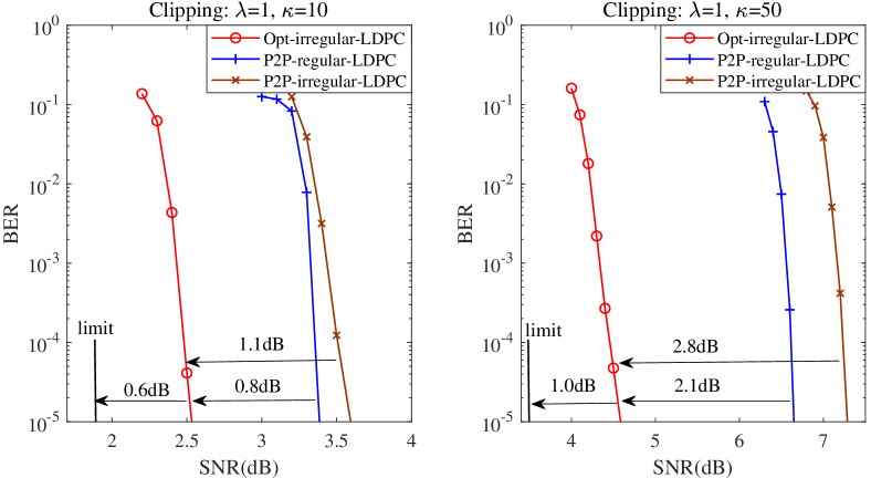
Note that the principle of optimal code design in Lemma 3 is applicable for arbitrary input distributions. Thus, we consider the practical LDPC code design for QPSK signaling with target rate $R_{\mathrm{sum}}=NR_{\mathrm{LDPC}}{\mathrm{log}}_{2}|\mathcal{S}_{\mathrm{QPSK}}|=500$, where $R_{\mathrm{LDPC}}$$=0.5$ and $|\mathcal{S}_{\mathrm{QPSK}}|$$=4$. Fig. 6 shows the gaps between BER curves at $10^{-4}$ of the optimized LDPC codes and the corresponding theoretical limits are about within $1.0$ dB, which verifies the near optimality of the proposed LDPC codes. Moreover, compared with P2P regular $(3,6)$ LDPC codes and well-designed irregular LDPC codes with $R_{\rm{LDPC}}=0.5$ [25], the optimized LDPC codes with GOAMP/GVAMP can achieve about $0.8\sim 2.8$ dB performance gains. The above comparison demonstrates that the Bayes optimal GOAMP/GVAMP cannot be guaranteed to achieve error-free performance.

References

- [1] J. Singh, O. Dabeer, and U. Madhow, “On the limits of communication with low-precision analog-to-digital conversion at the receiver,” IEEE Trans. Commun., vol. 57, no. 12, pp. 3629–3639, 2009.
- [2] S. Liang, J. Ma, and L. Ping, “Clipping can improve the performance of spatially coupled sparse superposition codes,” IEEE Commun. Lett., vol. 21, no. 12, pp. 2578–2581, 2017.
- [3] X. Yang, S. Jin, and C.-K. Wen, “Symbol detection of phase noise-impaired massive MIMO using approximate bayesian inference,” IEEE Signal Process. Lett., vol. 26, no. 4, pp. 607–611, 2019.
- [4] S. Wang, L. Zhang, and X. Jing, “Phase retrieval motivated nonlinear MIMO communication with magnitude measurements,” IEEE Trans. Wireless Commun., vol. 16, no. 8, pp. 5452–5466, 2017.
- [5] C.-J. Wang, C.-K. Wen, S.-H. Tsai, and S. Jin, “Decentralized expectation consistent signal recovery for phase retrieval,” IEEE Trans. Signal Proc., vol. 68, pp. 1484–1499, 2020.
- [6] O. Orhan, E. Erkip, and S. Rangan, “Low power analog-to-digital conversion in millimeter wave systems: Impact of resolution and bandwidth on performance,” in Proc. Inf. Theory Appl. Workshop (ITA), 2015, pp. 191–198.
- [7] L. Fan, S. Jin, C.-K. Wen, and H. Zhang, “Uplink achievable rate for massive MIMO systems with low-resolution ADC,” IEEE Commun. Lett., vol. 19, no. 12, pp. 2186–2189, 2015.
- [8] S. Liang, J. Tong, and L. Ping, “On iterative compensation of clipping distortion in OFDM systems,” IEEE Wireless Commun. Lett., vol. 8, no. 2, pp. 436–439, 2019.
- [9] S. Rangan, “Generalized approximate message passing for estimation with random linear mixing,” in Proc. IEEE Int. Symp. Inf. Theory Proc., 2011, pp. 2168–2172.
- [10] P. Schniter, S. Rangan, and A. K. Fletcher, “Vector approximate message passing for the generalized linear model,” in Proc. Asilomar Conf. on Signals, Systems, and Computers (Pacific Grove, CA), 2016, pp. 1525–1529.
- [11] P. Pandit, M. Sahraee-Ardakan, S. Rangan, P. Schniter, and A. K. Fletcher, “Inference with deep generative priors in high dimensions,” IEEE J. Sel. Areas Inf. Theory, vol. 1, no. 1, pp. 336–347, 2020.
- [12] L. Liu, S. Huang, and B. M. Kurkoski, “Memory AMP,” IEEE Trans. Inf. Theory, vol. 68, no. 12, pp. 8015–8039, 2022.
- [13] F. Tian, L. Liu, and X. Chen, “Generalized memory approximate message passing for generalized linear model,” IEEE Transactions on Signal Processing, vol. 70, pp. 6404–6418, 2022.
- [14] L. Liu, C. Liang, J. Ma, and L. Ping, “Capacity optimality of AMP in coded systems,” IEEE Trans. Inf. Theory, vol. 67, no. 7, pp. 4429–4445, 2021.
- [15] G. Reeves and H. D. Pfister, “The replica-symmetric prediction for random linear estimation with Gaussian matrices is exact,” IEEE Trans. Inf. Theory, vol. 65, no. 4, pp. 2252–2283, 2019.
- [16] J. Barbier, N. Macris, M. Dia, and F. Krzakala, “Mutual information and optimality of approximate message-passing in random linear estimation,” IEEE Trans. Inf. Theory, vol. 66, no. 7, pp. 4270–4303, 2020.
- [17] L. Liu, S. Liang, and L. Ping, “Capacity optimality of OAMP in coded large unitarily invariant systems,” Proc. 2022 IEEE Int. Symp. Inf. Theory (ISIT), arXiv preprint arXiv:2108.08503, pp. 1384–1389, 2022.
- [18] Y. Chi, L. Liu, G. Song, Y. Li, Y. L. Guan, and C. Yuen, “Constrained capacity optimal generalized multi-user MIMO: A theoretical and practical framework,” IEEE Trans. Commun., vol. 70, no. 12, pp. 8086–8104, 2022.
- [19] D. Guo, S. Shamai, and S. Verdu, “Mutual information and minimum mean-square error in Gaussian channels,” IEEE Trans. Inf. Theory, vol. 51, no. 4, pp. 1261–1282, 2005.
- [20] K. Takeuchi, “Rigorous dynamics of expectation-propagation-based signal recovery from unitarily invariant measurements,” IEEE Trans. Inf. Theory, vol. 66, no. 1, pp. 368–386, 2020.
- [21] J. R. Ebert, J.-F. Chamberland, and K. R. Narayanan, “On sparse regression LDPC codes,” arXiv preprint arXiv:2301.01899, 2023.
- [22] J. Tong, L. Ping, Z. Zhang, and V. K. Bhargava, “Iterative soft compensation for OFDM systems with clipping and superposition coded modulation,” IEEE Trans. Commun., vol. 58, no. 10, pp. 2861–2870, 2010.
- [23] A. M. Tulino and S. Verd, Random matrix theory and wireless communications. Commun.and Inf.theory, 2004.
- [24] J. Vila, P. Schniter, S. Rangan, F. Krzakala, and L. Zdeborov, “Adaptive damping and mean removal for the generalized approximate message passing algorithm,” in Proc. IEEE Int. Conf. Acoust., Speech Signal Process. (ICASSP), 2015, pp. 2021–2025.
- [25] T. Richardson, M. Shokrollahi, and R. Urbanke, “Design of capacity-approaching irregular low-density parity-check codes,” IEEE Trans. Inf. Theory, vol. 47, no. 2, pp. 619–637, 2001.
- [26] R. Berthier, A. Montanari, and P.-M. Nguyen, “State evolution for approximate message passing with non-separable functions,” Inf. Inference, A J. IMA, vol. 9, no. 1, pp. 33–79, 2020.
- [27] S. Rangan, P. Schniter, and A. K. Fletcher, “Vector approximate message passing,” IEEE Trans. Inf. Theory, vol. 65, no. 10, pp. 6664–6684, 2019.
Appendix A Orthogonality and Asymptotic IID Gaussianity
Define error vectors as