General-relativistic thin-shell
Dyson mega-spheres

Thomas Berry ¹, Alex Simpson ², Matt Visser ²

Abstract

Loosely inspired by the somewhat fanciful notion of detecting an arbitrarily advanced alien civilization, we consider a general-relativistic thin-shell Dyson mega-sphere completely enclosing a central star-like object, and perform a full general-relativistic analysis using the Israel–Lanczos–Sen junction conditions. We focus attention on the surface mass density, the surface stress, the classical energy conditions, and the quasi-local forces between hemispheres. We find that in the physically acceptable region the NEC, WEC, and SEC are always satisfied, while the DEC can be violated if the Dyson mega-sphere is sufficiently close to forming a black hole. We also demonstrate that the original quasi-local version of the maximum force conjecture, $F\leq{1\over 4}F_{Stoney}={1\over 4}F_{Planck}$ , can easily be violated if the Dyson mega-sphere is sufficiently compact, that is, sufficiently close to forming a black hole. Interestingly there is a finite region of parameter space where one can violate the original quasi-local version of the maximum force conjecture without violating the DEC. Finally, we very briefly discuss the possibility of nested thin-shell mega-spheres (Matrioshka configurations) and thick-shell Dyson mega-spheres.

Date: 6 July 2022; 16 September 2022; LaTeX-ed .

Keywords: Dyson mega-sphere; Kardashev type II civilization; general relativity; Israel–Lanczos–Sen junction conditions; classical energy conditions; Quasi-local maximum force conjecture; Matrioshka configurations; Matrioshka brain.

PhySH: Gravitation

This version accepted for publication in Physical Review D.

1 Introduction

In 1960 Freeman Dyson [1] mooted the idea that an arbitrarily advanced civilization, (at least a Kardashev type II civilization [2, 3]), might seek to control and utilize the energy output of an entire star by building a spherical mega-structure to completely enclose the star, trap all its radiant emissions, and use the energy flux to do “useful” work. Dyson’s idea has led to observational searches [4], extensive technical discussions [5], and more radical proposals such as reverse-Dyson configurations [6], (where one harvests the CMB and dumps waste heat into a central black hole), and “hairy” Dyson spheres [7], (with Gallileon “hair”). The vast majority of currently available analyses along these lines use Newtonian gravity, but herein we shall seek to perform an analysis in the thin-shell (Israel–Lanczos–Sen [8, 9, 10, 11, 12] junction condition) limit using standard general relativity.¹¹1Much more rarely one may sometimes encounter analyses using nonstandard theories of modified gravity [7]. For the current article, in the interests of tractability, we shall restrict attention to investigating systems with spherical symmetry.

For calculations we adopt geometrodynamic units where $G_{N}\to 1$ and $c\to 1$ , see for instance [13, 14]. Sometimes we will present key results in physical SI units, but when we do we shall explicitly say so. We furthermore adopt the sign conventions of [13, 14].

2 Spacetime metric ansatz

To set the stage, let the central star have mass $m$ , and take the mega-sphere to have a radius $a$ larger than the radius of the star; in fact for almost all purposes we may safely idealize the radius of the central star to be zero. Let the total mass of the (star)+(mega-sphere) system be $M$ . Then, outside the mega-sphere, the spacetime geometry can be described by

{\mathrm{d}}s^{2}=-\left(1-{2M\over r}\right){\mathrm{d}}t^{2}+{{\mathrm{d}}r^{2}\over 1-2M/r}+r^{2}\;{\mathrm{d}}\Omega^{2};\qquad(r>a);

(2.1)

while inside the mega-sphere

{\mathrm{d}}s^{2}=-\xi^{2}\left(1-{2m\over r}\right){\mathrm{d}}t^{2}+{{\mathrm{d}}r^{2}\over 1-2m/r}+r^{2}\;{\mathrm{d}}\Omega^{2}.\qquad(r<a);

(2.2)

Here to maintain continuity of the $t$ coordinate as one crosses the mega-sphere at $r=a$ it is useful to set

\xi^{2}={1-2M/a\over 1-2m/a}.

(2.3)

Physically we must demand $0\leq m\leq M<a/2$ . First we demand $m<a/2$ and $M<a/2$ to prevent horizon formation from enclosing the mega-sphere. Then we demand $M\geq m$ so that the total mass is not smaller than the mass of the central object. Finally $m\geq 0$ so that the central object does not have negative mass. Putting this all together we have $0\leq m\leq M<a/2$ , so that $0\leq\xi^{2}\leq 1$ .

It is furthermore useful to define a proper distance radial coordinate, normalized so that $\ell=0$ on the shell at $r=a$ :

\ell(r)=\left\{\begin{array}[]{l l}\displaystyle{+\int_{a}^{r}{{\mathrm{d}}r\over\sqrt{1-2M/r}}}&\qquad(r>a);\\[20.0pt] \displaystyle{-\int_{r}^{a}{{\mathrm{d}}r\over\sqrt{1-2m/r}}}&\qquad(r<a).\end{array}\right.

(2.4)

Then $n_{a}=\nabla_{a}\ell$ is by construction a unit outward-pointing spacelike vector, which we can use to define the projection operator

h_{ab}=g_{ab}-n_{a}\;n_{b}.

(2.5)

Finally, formally inverting $\ell(r)$ to implicitly extract $r(\ell)$ , one can re-express the spacetime geometry as

{\mathrm{d}}s^{2}=-\left(1-{2M\over r(\ell)}\right){\mathrm{d}}t^{2}+{{\mathrm{d}}\ell^{2}}+r(\ell)^{2}\;{\mathrm{d}}\Omega^{2};\qquad(r>a);

(2.6)

{\mathrm{d}}s^{2}=-\xi^{2}\left(1-{2m\over r(\ell)}\right){\mathrm{d}}t^{2}+{{\mathrm{d}}\ell^{2}}+r(\ell)^{2}\;{\mathrm{d}}\Omega^{2};\qquad(r<a).

(2.7)

3 Israel–Lanczos–Sen junction conditions

It is now straightforward to calculate the extrinsic curvature tensors

(K^{\pm})_{ab}={1\over 2}\left.{\partial g_{ab}\over\partial\ell}\right|_{\ell=0^{\pm}}={1\over 2}\left.{\partial r\over\partial\ell}\;{\partial g_{ab}\over\partial r}\right|_{\ell=0^{\pm}}={1\over 2}\left.{1\over\sqrt{g_{rr}}}\;{\partial g_{ab}\over\partial r}\right|_{\ell=0^{\pm}}

(3.1)

just above and below the thin shell at $r=a$ . (This calculation is well-known and can be found in very many places. See for instance references [8, 9, 10, 11, 12] and the more recent references [15, 16, 17, 18, 19].)

Then in the coordinate basis the extrinsic curvatures are:

(K^{+})_{tt}=-\sqrt{1-2M/a}\;{M\over a^{2}};\qquad(K^{+})_{\theta\theta}={(K^{+})_{\phi\phi}\over\sin^{2}\theta}=\sqrt{1-2M/a}\;a;

(3.2)

and

(K^{-})_{tt}=-\xi^{2}\sqrt{1-2m/a}\;{m\over a^{2}};\qquad(K^{-})_{\theta\theta}={(K^{-})_{\phi\phi}\over\sin^{2}\theta}=\sqrt{1-2m/a}\;a.

(3.3)

Rewriting this in the natural orthonormal basis one has:

(K^{+})_{\hat{t}\hat{t}}=-{M/a^{2}\over\sqrt{1-2M/a}};\qquad(K^{+})_{\hat{\theta}\hat{\theta}}=(K^{+})_{\hat{\phi}\hat{\phi}}={\sqrt{1-2M/a}\over a};

(3.4)

and

(K^{-})_{\hat{t}\hat{t}}=-{m/a^{2}\over\sqrt{1-2m/a}};\qquad(K^{-})_{\hat{\theta}\hat{\theta}}=(K^{-})_{\hat{\phi}\hat{\phi}}={\sqrt{1-2m/a}\over a}.

(3.5)

Furthermore, the (distributional) stress-energy on the shell is then easily obtained in terms of the discontinuity $[K]_{ab}$ of the extrinsic curvatures [8, 9, 10, 11, 12, 15, 16, 17, 18, 19]

[K]_{ab}=(K_{+})_{ab}-(K_{-})_{ab}.

(3.6)

Explicitly, working in the natural orthonormal basis,

[K]_{\hat{a}\hat{b}}=\left[\begin{array}[]{cc|cc}-{M/a^{2}\over\sqrt{1-2M/a}}+{m/a^{2}\over\sqrt{1-2m/a}}&0&0&0\\[10.0pt] 0&0&0&0\\[1.0pt] \hline\cr 0&0&{\vphantom{\Bigg{|}}{\sqrt{1-2M/a}\over a}}-{\sqrt{1-2m/a}\over a}&0\\ 0&0&0&{\sqrt{1-2M/a}\over a}-{\sqrt{1-2m/a}\over a}\end{array}\right].

(3.7)

For the discontinuity in the trace of the extrinsic curvature, $K=g^{ab}K_{ab}=g^{\hat{a}\hat{b}}K_{\hat{a}\hat{b}}$ , we have

[K]=+{M/a^{2}\over\sqrt{1-2M/a}}-{m/a^{2}\over\sqrt{1-2m/a}}+2\left({\sqrt{1-2M/a}\over a}-{\sqrt{1-2m/a}\over a}\right),

(3.8)

which can be re-written as

[K]=+{1\over a}\left\{{2-3M/a\over\sqrt{1-2M/a}}-{2-3m/a\over\sqrt{1-2m/a}}\right\}.

(3.9)

By invoking the Israel–Lanczos–Sen junction conditions, ([8, 9, 10, 11, 12], see also [15, 16, 17, 18, 19]), we find the distributional stress-energy tensor:

T_{ab}=-{1\over 8\pi}\left([K]_{ab}-[K]h_{ab}\right)\,\delta(\ell)=S_{ab}\;\delta(\ell),

(3.10)

or better yet, its orthonormal form:

T_{\hat{a}\hat{b}}=-{1\over 8\pi}\left([K]_{\hat{a}\hat{b}}-[K]h_{\hat{a}\hat{b}}\right)\,\delta(\ell)=S_{\hat{a}\hat{b}}\;\delta(\ell).

(3.11)

Here $\ell$ is the proper radial distance from the shell, as defined in equation (2.4). Furthermore we define the surface energy density $\sigma$ , and surface stress $\Pi$ (this is the negative of what is usually called the surface tension $\vartheta$ , that is, $\Pi=-\vartheta$ ) by

S_{\hat{a}\hat{b}}=\left[\begin{array}[]{cc|cc}\sigma&0&0&0\\ 0&0&0&0\\ \hline\cr 0&0&\Pi&0\\ 0&0&0&\Pi\end{array}\right].

(3.12)

Thence

\sigma={1\over 4\pi\,a}\;\left(\sqrt{1-2m/a}-\sqrt{1-2M/a}\right),

(3.13)

and

\Pi={1\over 8\pi\,a}\left({1-M/a\over\sqrt{1-2M/a}}-{1-m/a\over\sqrt{1-2m/a}}\right).

(3.14)

Now, as long as $M\geq m$ , it is immediate that the surface energy density is positive, $\sigma\geq 0$ . To bound the surface stress $\Pi$ , we note that

{\partial\Pi\over\partial M}={M\over 8\pi\,a^{3}(1-2M/a)^{3/2}}>0.

(3.15)

Thence, as long as we satisfy the physically motivated constraint that $M\geq m$ , (the total mass of the system is greater than the mass of the central star), it is immediate that $\Pi\geq 0$ . So in the physically relevant regime, where $a>2M\geq 2m\geq 0$ , all the surface stress-energy components are guaranteed non-negative.

Somewhat similar calculations are relevant to thin-shell gravastar models [20, 21, 22, 23], though in that context many of the technical details, and all of the physics goals, are very different.

4 Classical energy conditions

4.1 Definitions

For any type I stress energy tensor [24], (which is certainly and explicitly the case in the current spherically symmetric situation), the standard classical energy conditions are based on considering various linear combinations of the energy density $\rho$ and the principal pressures $p_{i}$ . (See primarily references [25, 26, 27, 28, 29, 30], but see also references [31, 32, 33, 34] and [35, 36, 37, 38, 39, 40, 41, 42].)

NEC:: $\rho+p_{i}\geq 0$ .
WEC:: $\rho\geq 0$ and $\rho+p_{i}\geq 0$ .
SEC:: $\rho+\sum_{i}p_{i}\geq 0$ and $\rho+p_{i}\geq 0$ .
DEC:: $|p_{i}|\leq\rho$ .

Thence, in this specific thin-shell configuration, with principal stresses of the form $\mathrm{diag}\{\sigma,0,\Pi,\Pi\}$ , these standard classical energy conditions will specialize to:

NEC:: $\sigma\geq 0$ and $\sigma+\Pi\geq 0$ .
WEC:: Equivalent to NEC.
SEC:: NEC and $\sigma+2\Pi\geq 0$ .
DEC:: NEC and $\sigma-\Pi\geq 0$ . (That is, $|\Pi|\leq\sigma$ .)

We shall now analyze these energy conditions in detail.

4.2 Null, weak, and strong energy conditions

In the physically relevant regime, $M\geq m$ , both $\sigma$ and $\Pi$ are guaranteed non-negative, so all three of the NEC, WEC, and SEC are automatically satisfied.

4.3 Dominant energy condition

To investigate the DEC it is useful to define the dimensionless quantity

w={\Pi\over\sigma},

(4.1)

and ask whether or not $w\leq 1$ . (We already know $w\geq 0$ .)

Explicitly, to investigate the DEC we see that we need to consider the dimensionless parameter

w={1\over 2}{\left({1-M/a\over\sqrt{1-2M/a}}-{1-m/a\over\sqrt{1-2m/a}}\right)\over\left(\sqrt{1-2m/a}-\sqrt{1-2M/a}\right)}

(4.2)

This quantity is more easily analyzed in terms of two dimensionless “compactness” parameters $\mbox{\Large$\chi$}=2M/a$ and $\chi=2m/a$ , where now the physically acceptable range corresponds to $0\leq\chi\leq\mbox{\Large$\chi$}\leq 1$ . Then,

w={1\over 2}{\left({1-\mbox{\Large$\chi$}/2\over\sqrt{1-\mbox{\Large$\chi$}}}-{1-\chi/2\over\sqrt{1-\chi}}\right)\over\left(\sqrt{1-\chi}-\sqrt{1-\mbox{\Large$\chi$}}\right)}={1\over 4}\left\{{1\over\sqrt{1-\chi}\sqrt{1-\mbox{\Large$\chi$}}}-1\right\}.

(4.3)

Saturation of the DEC, the condition $w=1$ , then easily translates to

(1-\mbox{\Large$\chi$})(1-\chi)={1\over 25}.

(4.4)

Less symmetrically, but perhaps more usefully, this can be rewritten as

\chi=1-{1\over 25(1-\mbox{\Large$\chi$})};\qquad\qquad\mbox{\Large$\chi$}=1-{1\over 25(1-\chi)}.

(4.5)

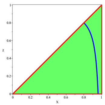
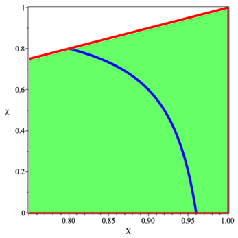
For a thin-shell Dyson mega-sphere on the verge of violating the DEC we have

\sigma=\Pi={1\over 4\pi\,a}\;\left(\sqrt{1-\chi}-\sqrt{1-\mbox{\Large$\chi$}}\right)={1\over 4\pi\,a}\;\left({1\over 5\sqrt{1-\mbox{\Large$\chi$}}}-\sqrt{1-\mbox{\Large$\chi$}}\right).

(4.6)

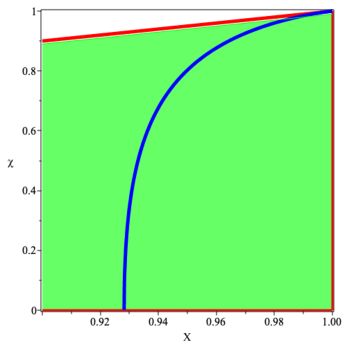
To enforce $\sigma\geq 0$ while saturating the DEC one needs $\mbox{\Large$\chi$}\geq 4/5$ , (and $\mbox{\Large$\chi$}<1$ ).

Furthermore, the DEC-violating region is easily seen to be

1-{1\over 25(1-\mbox{\Large$\chi$})}<\chi<\mbox{\Large$\chi$}\leq 1.

(4.7)

That is

{{24\over 25}-\mbox{\Large$\chi$}\over 1-\mbox{\Large$\chi$}}<\chi<\mbox{\Large$\chi$}\leq 1.

(4.8)

Thus violations of the DEC are relatively easy to arrange. (At least theoretically; the implied construction materials would be somewhat outré.) It should be emphasized that violations of the classical energy conditions are not absolute prohibitions on “interesting physics”, see [25, 26, 27] and specifically [41, 42, 43], but they certainly are invitations to think very carefully about the underlying physics.

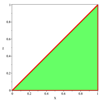
The three regions where $w<1$ , $w=1$ , and $w>1$ in the physically acceptable part of the $(\chi,\mbox{\Large$\chi$})$ plane, $0\leq\chi\leq\mbox{\Large$\chi$}\leq 1$ , are plotted in figures 1–3.

Refer to caption — Figure 1: Boundary and interior of the physically acceptable region $0\leq\chi\leq\mbox{\Large$\chi$}<1$ .

5 Quasi-local forces

Whenever one is dealing with an extended object in general relativity, (star, planet, Dyson mega-sphere), the notion of “force” is at best a quasi-local concept associated with some region and its boundary. For a static bulk region with boundary 2-surface $\Sigma$ it is natural to use the induced 2-metric $(g_{2})_{ij}$ , and the normal $n^{a}$ to $\Sigma$ , to define

F_{\Sigma}=\int_{\Sigma}(T_{ab}\,n^{a}n^{b})\,\sqrt{g_{2}}\,{\mathrm{d}}^{2}x=\int_{\Sigma}p_{\perp}\;{\mathrm{d}}A.

(5.1)

For a static thin-shell region (a 2-surface) with boundary 1-surface $L$ it is natural to use the induced 1-metric $(g_{1})$ on $L$ , and the within-shell normal $n^{a}$ to the curve $L$ , to define

F_{L}=\int_{L}(T_{ab}\,n^{a}n^{b})\,\sqrt{g_{1}}\,{\mathrm{d}}x=\int_{L}\Pi_{\perp}\;{\mathrm{d}}L.

(5.2)

These quasi-local forces were the impetus for original quasi-local versions of the maximum force conjecture, now thoroughly disproved by a number of explicit counter-examples [44]. It is only for point-like objects that any “ultra-local” notion of force can meaningfully be formulated, and in the current context (working with Dyson mega-spheres) it is clear that the quasi-local notion of force is primary.

5.1 Quasi-local force between two hemispheres

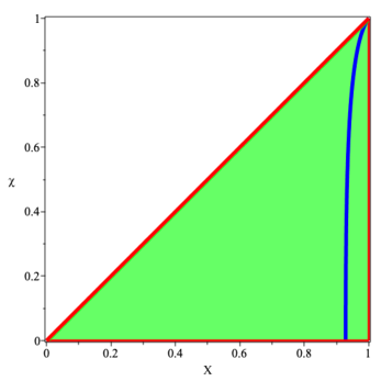
The quasi-local force between any two hemispheres separated by a great circle on the Dyson mega-sphere is simply given (in the usual geometrodynamic units) by the dimensionless quantity

F=\Pi\times(2\pi a)={1\over 4}\left({1-M/a\over\sqrt{1-2M/a}}-{1-m/a\over\sqrt{1-2m/a}}\right).

(5.3)

We first rewrite this in terms of the two dimensionless compactness parameters, $\mbox{\Large$\chi$}=2M/a$ and $\chi=2m/a$ , as

F={1\over 4}\left({1-\mbox{\Large$\chi$}/2\over\sqrt{1-\mbox{\Large$\chi$}}}-{1-\chi/2\over\sqrt{1-\chi}}\right).

(5.4)

This can further be recast as

F={1\over 8}\left({1\over\sqrt{1-\mbox{\Large$\chi$}}}+\sqrt{1-\mbox{\Large$\chi$}}-{1\over\sqrt{1-\chi}}-\sqrt{1-\chi}\right).

(5.5)

The maximum original quasi-local force conjecture, in its strong form, would require $F\leq 1/4$ . But this is easily seen to be generically violated; see discussion below.

5.2 Physical units

To rephrase this discussion in physical units, let us consider the Stoney force [45, 46, 47], (also known as the Planck force, though the analysis by Stoney pre-dates that of Planck by some 20 years [48]). This is defined by

F_{Stoney}=F_{Planck}={c^{4}\over G_{N}}\approx 1.2\times 10^{44}\hbox{ N},

(5.6)

in terms of which, re-inserting the factors of $c$ and $G_{N}$ as in (5.6), one has

F_{physical}={1\over 4}\left({1-\mbox{\Large$\chi$}/2\over\sqrt{1-\mbox{\Large$\chi$}}}-{1-\chi/2\over\sqrt{1-\chi}}\right)F_{Stoney}.

(5.7)

Alternatively,

F_{physical}={1\over 8}\left({1\over\sqrt{1-\mbox{\Large$\chi$}}}+\sqrt{1-\mbox{\Large$\chi$}}-{1\over\sqrt{1-\chi}}-\sqrt{1-\chi}\right)F_{Stoney}.

(5.8)

5.3 Special case $m=0$

We first note that

{\partial F\over\partial M}={M\over 4a^{2}(1-2M/a)^{3/2}}>0;

(5.9)

and

{\partial F\over\partial m}=-{m\over 4a^{2}(1-2m/a)^{3/2}}<0.

(5.10)

So to maximize the quasi-local force between any two hemispheres one should maximize $M$ , (without forming a black hole, so one requires $M<a/2$ ), and minimize $m$ , (for instance by setting $m\to 0$ , so that the Dyson mega-sphere is empty, there is no central star).

It is then easy to check that for the special case $m=0$ we have

F_{m=0}={1\over 4}\left({1-M/a\over\sqrt{1-2M/a}}-1\right)={1\over 4}\left({1-\mbox{\Large$\chi$}/2\over\sqrt{1-\mbox{\Large$\chi$}}}-1\right).

(5.11)

Therefore, when forcing $m=0$ , we certainly have $F_{m=0}>1/4$ over the entire range

\mbox{\Large$\chi$}\in\Big{(}\left\{4\sqrt{3}-6\right\},1\Big{)}=\Big{(}0.928203232...,1\Big{)}.

(5.12)

Thence, in this Dyson mega-sphere setting, sufficiently close to black hole formation the original quasi-local form of the maximum force conjecture is manifestly false. If one desires to rescue the the maximum force conjecture one needs to redefine the notion of force in an “ultra-local” manner, by carefully (and somewhat artificially) restricting the domain of discourse to only include certain “ultra-local” forces relevant to point-particle situations, and not relevant for extended objects. It is only for such a redefined “ultra-local” maximum force conjecture that there is any chance of getting it to work. See related discussion in references [44, 49, 50], with countervailing opinions in references [51, 52].

5.4 General case

More generally in terms of the two compactness parameters $\chi$ and $\chi$ , we have already seen:

	$\displaystyle F$	$\displaystyle=$	$\displaystyle{1\over 4}\left({1-\mbox{\Large$\chi$}/2\over\sqrt{1-\mbox{\Large$\chi$}}}-{1-\chi/2\over\sqrt{1-\chi}}\right)$		(5.13)
		$\displaystyle=$	$\displaystyle{1\over 8}\left({1\over\sqrt{1-\mbox{\Large$\chi$}}}+\sqrt{1-\mbox{\Large$\chi$}}-{1\over\sqrt{1-\chi}}-\sqrt{1-\chi}\right).$		(5.14)

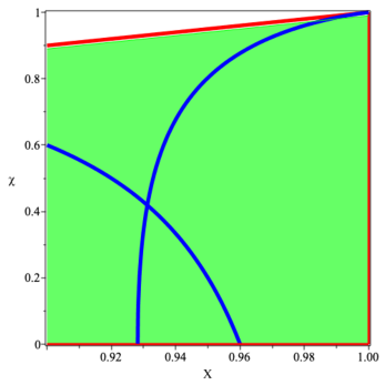
For any fixed value of $\chi$ , this force $F$ becomes arbitrarily large as $\mbox{\Large$\chi$}\to 1$ . Specifically, the boundary of the region satisfying both $F<1/4$ and the physicality constraints $0\leq\chi\leq\mbox{\Large$\chi$}\leq 1$ is plotted in figures 4 and 5.²²2 To obtain the curved line in figures 4 and 5 one sets $F=1/4$ and solves resulting quadratic for $\chi$ as a function of $\chi$ . This quadratic yields two somewhat messy roots, only one of which is physical. Even then, one has to be careful to restrict attention to the physically relevant region.

Again, we see that the original quasi-local form of the maximum force conjecture is manifestly false. For this quasi-local maximum force violation to occur one must be “close” to black hole formation $\chi\lesssim\mbox{\Large$\chi$}\lesssim 1$ .

6 Violating the quasi-local maximum force conjecture — without violating the DEC

By superimposing the parts of the physical regime $0\leq\chi\leq\mbox{\Large$\chi$}\leq 1$ where both $w<1$ and $F>1/4$ one easily sees that it is possible to violate the (strong) maximum force conjecture without violating the DEC. See figure 6. It is also possible to violate the DEC while satisfying the (strong) maximum force conjecture. For this to occur one must be “close” to black hole formation $\chi\lesssim\mbox{\Large$\chi$}\lesssim 1$ .

7 Weak-gravity regime

In the weak-gravity regime, (where both $\mbox{\Large$\chi$}=2M/a\ll 1$ and $\chi=2m/a\ll 1$ ), we have

\sigma\approx{1\over 4\pi}{M-m\over a^{2}}\geq 0,

(7.1)

and

\Pi\approx{1\over 16\pi}{M^{2}-m^{2}\over a^{3}}\geq 0.

(7.2)

So in the weak-gravity regime one has the physically plausible result that

M\approx m+4\pi\sigma\,a^{2},

(7.3)

while the surface stress is

\Pi\approx{1\over 4}\;{(M+m)\over a}\;\sigma\;\ll\;\sigma.

(7.4)

That is

w={\Pi\over\sigma}\approx{1\over 4}\;{(M+m)\over a}={\mbox{\Large$\chi$}+\chi\over 8}\;\;\ll\;1.

(7.5)

So all the classical energy conditions, including the DEC, are automatically satisfied in the weak-gravity regime.

Finally note that in the weak gravity regime the force between two hemispheres is

F\approx{1\over 8}\;{M^{2}-m^{2}\over a^{2}}={1\over 2}(\mbox{\Large$\chi$}^{2}-\chi^{2})\ll 1.

(7.6)

However, we have seen above that we have much more general and precise results available, fully applicable to the highly relativistic strong-gravity regime.

8 Low-mass thin-shell configurations

Another interesting approximation is that of a low-mass thin-shell, where

M-m\ll m.

(8.1)

We can then approximate

\sigma(m,M;a)={M-m\over 4\pi a^{2}\sqrt{1-2M/a}}+\mathcal{O}([M-m]^{2}),

(8.2)

while

\Pi(m,M;a)={m(M-m)\over 8\pi a^{3}\sqrt{1-2M/a}}+\mathcal{O}([M-m]^{2}).

(8.3)

Partially eliminating $M-m$ between these two equations we see

\Pi(m,M;a)={1\over 4}\;{2m\over a}\;\sigma(m,M;a)+\mathcal{O}([M-m]^{2}).

(8.4)

Trivially,

w(m,M;a)={m/a\over 2(1-2m/a)}+\mathcal{O}([M-m]),

(8.5)

and

F(m,M;a)={m(M-m)\over a^{2}\sqrt{1-2M/a}}+\mathcal{O}([M-m]^{2}),

(8.6)

while with a little more work we can obtain

w(m,M;a)={m/a\over 2(1-2m/a)}+{(M-m)\over 4a(1-2m/a)^{2}}+\mathcal{O}([M-m]^{2}).

(8.7)

Thus even for a low mass shell, $M-m\ll m$ , by driving $\chi\to 1$ , one can still easily arrange violations of the DEC and the original form of the maximum force conjecture.

To calibrate the approximate size of these quantities note that in geometrodynamic units the mass of our Sun is $M_{\odot}\approx 1.5\;\hbox{km}$ , while the mass of Jupiter is $M_{\text{\char 88\relax}}\approx 1.1\;\hbox{m}$ . The astronomical unit is $1\;\hbox{AU}\approx 1.5\times 10^{8}\;\hbox{km}$ . Then disassembling Jupiter to build a mega-sphere with radius 1 AU leads to the dimensionless estimates

w\approx 5\times 10^{-9};\qquad F\approx 7.333\times 10^{-20}.

(8.8)

That is, solar system scale Dyson mega-spheres would be well into the Newtonian regime. For general relativistic effects to be appreciable one must be “close” to black hole formation $\chi\lesssim\mbox{\Large$\chi$}\lesssim 1$ .

Furthermore in physical units we have $M_{\text{\char 88\relax}}\approx 1.898\times 10^{27}\;\hbox{kg}$ , so that for the surface energy density

\sigma\approx{M_{\text{\char 88\relax}}\over(4\pi\,1\,{\hbox{AU}}^{2})}\approx 7003\;\hbox{kg/m}^{2}.

(8.9)

Locally, this is actually human scale — since the density of iron is $\approx 7800\;\hbox{kg/m}^{3}$ , this would correspond to a Dyson mega-sphere a little under 1 metre thick. Globally speaking however, this is well beyond human technology, and would at the very least require the intervention of a Kardashev type II civilization [2, 3].

9 Possible generalizations

9.1 Matrioshka configurations

It would in principle be possible to extend the current discussion to deal with the more general Matrioshka configurations (multiply nested thin-shell Dyson mega-spheres). Such configurations have been mooted in the context of Matrioshka brains [53]. No really new matters of principle would be involved, but the algebra would become considerably more complex. We put such issues aside for now.

9.2 Thick-shell Dyson mega-spheres

In contrast potential consideration of thick-shell Dyson mega-spheres would require a completely different set of techniques — one would need to study the anisotropic Tolman–Oppenheimer–Volkoff (TOV) equation, paying careful attention to suitable boundary conditions and equations of state. We put such issues aside for now.

9.3 Adding rotation

Adding rotation to these Dyson mega-sphere configurations would likely be extremely tedious, if not outright impractical. Even if the angular momentum of the central object and Dyson mega-sphere are parallel, the required calculations would be daunting. One could either try to work with the full Kerr geometry [54, 55, 56, 57, 58, 59], or with the Lense–Thirring slow rotation approximation [60, 61, 62, 63, 64, 65]. We put such issues aside for now.

10 Conclusions

Arbitrarily advanced alien civilizations are the sine qua non of much speculative physics — developed with a view to testing the ultimate limitations of putative technological advancement. Notable examples of speculative physics are Dyson mega-structures, (specifically the Dyson mega-spheres of the current article), Lorentzian wormholes, warp drives, and tractor/pressor/stressor beams. A common theme arising in such speculative physics is the violation of some or all of the classical energy conditions, and/or violations of the original strong form of the maximum force conjecture. Such violations are not the absolute prohibition they were once thought to be, but they are certainly invitations to think deeply about the underlying physics.

The Dyson mega-structures in particular, are in principle accessible to astronomical observational tests. In the current article we have analyzed the simple spherically symmetric thin-shell Dyson mega-sphere, and have done so in a fully general relativistic manner using the Israel–Lanczos–Sen thin-shell formalism. We have seen that there are regions in parameter-space where either, both, or neither of the DEC and strong maximum quasi-local force conjecture are violated.

Acknowledgements

TB was indirectly supported by the Marsden Fund, via a grant administered by the Royal Society of New Zealand.
AS was supported by a Victoria University of Wellington PhD scholarship, and was also indirectly supported by the Marsden Fund, via a grant administered by the Royal Society of New Zealand.
MV was directly supported by the Marsden Fund, via a grant administered by the Royal Society of New Zealand.

References

[1] F. J. Dyson, “Search for Artificial Stellar Sources of Infrared Radiation”,
Science 131 # 3414 (1960) 1667–1668. doi:10.1126/science.131.3414.1667
[2] Nikolai Kardashev, “Transmission of Information by Extraterrestrial Civilizations”, Soviet Astronomy. 8 (1964) 217–221.
[3] Kardashev scale. See https://en.wikipedia.org/wiki/Kardashev_scale
[4] R. A. Carrigan, Jr., “IRAS-based whole-sky upper limit on Dyson Spheres”, Astrophys. J. 698 (2009), 2075-2086 doi:10.1088/0004-637X/698/2/2075 [arXiv: 0811.2376 [astro-ph]].
[5] T. Y. Y. Hsiao, T. Goto, T. Hashimoto, D. J. D. Santos, A. Y. L. On, E. Kilerci-Eser, Y. H. V. Wong, S. J. Kim, C. K. W. Wu and S. C. C. Ho, et al.
“A Dyson sphere around a black hole”, Mon. Not. Roy. Astron. Soc. 506 (2021) no.2, 1723-1732 doi:10.1093/mnras/stab1832 [arXiv: 2106.15181 [astro-ph.HE]].
[6] T. Opatrný, L. Richterek and P. Bakala, “Life under a black sun”,
Am. J. Phys. 85 (2017), 14 doi:10.1119/1.4966905 [arXiv: 1601.02897 [gr-qc]].
[7] N. Kaloper, A. Padilla and N. Tanahashi, “Galileon Hairs of Dyson Spheres, Vainshtein’s Coiffure and Hirsute Bubbles”, JHEP 10 (2011), 148 doi:10.1007/JHEP10(2011)148 [arXiv: 1106.4827 [hep-th]].
[8] W. Israel, “Singular hypersurfaces and thin shells in general relativity”, Nuovo Cim. B 44S10 (1966), 1 [erratum: Nuovo Cim. B 48 (1967), 463] doi:10.1007/BF02710419
[9] C. Barrabes and W. Israel, “Thin shells in general relativity and cosmology: The Lightlike limit”, Phys. Rev. D 43 (1991), 1129-1142 doi:10.1103/PhysRevD.43.1129
[10] Kornel Lanczos, “Flächenhafte Verteilung der Materie in der Einsteinschen Gravitationstheorie”, Annalen der Physik 379 #14 (1924) 518–540 doi:10.1002/andp.19243791403
[11] Korenel Lanczos, “Untersuching über flächenhafte verteilung der materie in der Einsteinschen Gravitationstheorie”, unpublished, 1922.
[12] Nikhilranjan Sen, Über die Grenzbedingungen des Schwerefeldes an Unstetigkeitsflächen”, Annalen der Physik 378 # 5-6 (1924) 365–396. doi:10.1002/andp.19243780505
[13] C. W. Misner, K. S. Thorne and J. A. Wheeler, Gravitation,
(Freeman, San Francisco, 1973).
[14] R. M. Wald, General Relativity, (U Chicago Press, Chicago, 1984), doi:10.7208/chicago/9780226870373.001.000.
[15] M. Visser, Lorentzian wormholes: From Einstein to Hawking,
(AIP Press; now Springer, Reading, 1996).
[16] M. Visser, “Traversable wormholes: Some simple examples”, Phys. Rev. D 39 (1989), 3182-3184 doi:10.1103/PhysRevD.39.3182 [arXiv: 0809.0907 [gr-qc]].
[17] M. Visser, “Traversable wormholes from surgically modified Schwarzschild space-times”, Nucl. Phys. B 328 (1989), 203-212 doi:10.1016/0550-3213(89)90100-4 [arXiv: 0809.0927 [gr-qc]].
[18] E. Poisson and M. Visser, “Thin shell wormholes: Linearization stability”,
Phys. Rev. D 52 (1995), 7318-7321 doi:10.1103/PhysRevD.52.7318 [arXiv: gr-qc/9506083 [gr-qc]].
[19] F. S. N. Lobo, M. Bouhmadi-López, P. Martín-Moruno, N. Montelongo-García and M. Visser, “A novel approach to thin-shell wormholes and applications,” doi:10.1142/9789813226609_0154 [arXiv: 1512.08474 [gr-qc]].
[20] M. Visser and D. L. Wiltshire, “Stable gravastars: An alternative to black holes?”, Class. Quant. Grav. 21 (2004), 1135-1152 doi:10.1088/0264-9381/21/4/027 [arXiv: gr-qc/0310107 [gr-qc]].
[21] P. Martín-Moruno, N. Montelongo-García, F. S. N. Lobo and M. Visser,
“Generic thin-shell gravastars”, JCAP 03 (2012) 034 doi:10.1088/1475-7516/2012/03/034 [arXiv: 1112.5253 [gr-qc]].
[22] F. S. N. Lobo, P. Martín-Moruno, N. Montelongo-García and M. Visser,
“Novel stability approach of thin-shell gravastars”, doi:10.1142/9789813226609_0221 [arXiv: 1512.07659 [gr-qc]].
[23] F. S. N. Lobo, P. Martín-Moruno, N. Montelongo-García and M. Visser,
“Linearised stability analysis of generic thin shells”, doi:10.1142/9789814623995_0321 [arXiv: 1211.0605 [gr-qc]].
[24] S. W. Hawking and G. F. R. Ellis, The Large Scale Structure of Space-Time, (Cambridge University Press, Cambridge, 1973), doi:10.1017/CBO9780511524646
[25] C. Barceló and M. Visser, “Twilight for the energy conditions?”,
Int. J. Mod. Phys. D 11 (2002), 1553-1560 doi:10.1142/S0218271802002888 [arXiv: gr-qc/0205066 [gr-qc]].
[26] E. Curiel, “A Primer on Energy Conditions”, Einstein Stud. 13 (2017), 43-104 doi:10.1007/978-1-4939-3210-8_3 [arXiv: 1405.0403 [physics.hist-ph]].
[27] E. A. Kontou and K. Sanders, “Energy conditions in general relativity and quantum field theory”, Class. Quant. Grav. 37 (2020) no.19, 193001 doi:10.1088/1361-6382/ab8fcf [arXiv: 2003.01815 [gr-qc]].
[28] A. D. Helfer, “Operational energy conditions”, Class. Quant. Grav. 15 (1998), 1169-1183 doi:10.1088/0264-9381/15/5/008 [arXiv: gr-qc/9709047 [gr-qc]].
[29] M. Alcubierre and F. S. N. Lobo, “Wormholes, Warp Drives and Energy Conditions”, Fundam. Theor. Phys. 189 (2017), pp.-279 doi:10.1007/978-3-319-55182-1 [arXiv: 2103.05610 [gr-qc]].
[30] F. S. N. Lobo and M. Visser, “Linearized warp drive and the energy conditions,” [arXiv: gr-qc/0412065 [gr-qc]].
(Contribution to ERE-2004, Madrid, September 2004.)
[31] M. Visser, “Energy conditions in the epoch of galaxy formation”, Science 276 (1997), 88-90 doi:10.1126/science.276.5309.88 [arXiv: 1501.01619 [gr-qc]].
[32] M. Visser, “General relativistic energy conditions: The Hubble expansion in the epoch of galaxy formation”, Phys. Rev. D 56 (1997), 7578-7587 doi:10.1103/PhysRevD.56.7578 [arXiv: gr-qc/9705070 [gr-qc]].
[33] M. Visser and C. Barceló, “Energy conditions and their cosmological implications”, doi:10.1142/9789812792129_0014, [arXiv: gr-qc/0001099 [gr-qc]].
[34] M. Visser, S. Kar and N. Dadhich, “Traversable wormholes with arbitrarily small energy condition violations”, Phys. Rev. Lett. 90 (2003), 201102 doi:10.1103/PhysRevLett.90.201102 [arXiv: gr-qc/0301003 [gr-qc]].
[35] P. Martín-Moruno and M. Visser, “Semiclassical energy conditions for quantum vacuum states”, JHEP 09 (2013), 050 doi:10.1007/JHEP09(2013)050 [arXiv: 1306.2076 [gr-qc]].
[36] P. Martín-Moruno and M. Visser, “Classical and quantum flux energy conditions for quantum vacuum states”, Phys. Rev. D 88 (2013) no.6, 061701 doi:10.1103/PhysRevD.88.061701 [arXiv: 1305.1993 [gr-qc]].
[37] P. Martín-Moruno and M. Visser, “Semi-classical and nonlinear energy conditions”, doi:10.1142/9789813226609_0126 [arXiv: 1510.00158 [gr-qc]].
(Contribution to MG14, Rome, July 2015).
[38] P. Martín-Moruno and M. Visser, “Classical and semi-classical energy conditions”, Fundam. Theor. Phys. 189 (2017), 193-213 doi:10.1007/978-3-319-55182-1_9 [arXiv: 1702.05915 [gr-qc]].
[39] P. Martín-Moruno and M. Visser, “Generalized Rainich conditions, generalized stress-energy conditions, and the Hawking-Ellis classification”, Class. Quant. Grav. 34 (2017) no.22, 225014 doi:10.1088/1361-6382/aa9039 [arXiv: 1707.04172 [gr-qc]].
[40] P. Martín-Moruno and M. Visser, “Hawking-Ellis classification of stress-energy tensors: Test fields versus backreaction”, Phys. Rev. D 103 (2021) no.12, 124003 doi:10.1103/PhysRevD.103.124003 [arXiv: 2102.13551 [gr-qc]].
[41] J. Santiago, S. Schuster and M. Visser,
“Generic warp drives violate the null energy condition”,
Phys. Rev. D 105 (2022) no.6, 064038 doi:10.1103/PhysRevD.105.064038 [arXiv: 2105.03079 [gr-qc]].
[42] J. Santiago, S. Schuster and M. Visser,
“Tractor Beams, Pressor Beams and Stressor Beams in General Relativity”,
Universe 7 (2021) no.8, 271 doi:10.3390/universe7080271 [arXiv: 2106.05002 [gr-qc]].
[43] M. Visser, J. Santiago and S. Schuster,
“Tractor beams, pressor beams, and stressor beams within the context of general relativity”, [arXiv: 2110.14926 [gr-qc]]. Contribution to MG16 (Rome, 2021).
[44] A. Jowsey and M. Visser, “Counterexamples to the Maximum Force Conjecture”, Universe 7 (2021) no.11, 403 doi:10.3390/universe7110403
[arXiv: 2102.01831 [gr-qc]].
[45] Stoney units. See https://en.wikipedia.org/wiki/Stoney_units
[46] G. Johnstone Stoney, “On The Physical Units of Nature”,
Phil.Mag. 11 (1881) 381–391.
[47] G. Johnstone Stoney, “On The Physical Units of Nature”,
Scientific Proceedings of the Royal Dublin Society, 3 (1883) 51–60.
[48] Planck units. See https://en.wikipedia.org/wiki/Planck_units
[49] A. Jowsey and M. Visser, “Reconsidering maximum luminosity”,
Int. J. Mod. Phys. D 30 (2021) no.14, 2142026 doi:10.1142/S0218271821420268 [arXiv: 2105.06650 [gr-qc]].
[50] V. Faraoni, “Maximum force and cosmic censorship”, Phys. Rev. D 103 (2021) no.12, 124010 doi:10.1103/PhysRevD.103.124010 [arXiv: 2105.07929 [gr-qc]].
[51] C. Schiller, “Comment on “Maximum force and cosmic censorship”’́,,
Phys. Rev. D 104 (2021) no.6, 068501 doi:10.1103/PhysRevD.104.068501 [arXiv: 2109.07700 [gr-qc]].
[52] C. Schiller, “Tests for maximum force and maximum power”,
Phys. Rev. D 104 (2021) no.12, 124079 doi:10.1103/PhysRevD.104.124079 [arXiv: 2112.15418 [gr-qc]].
[53] Matrioshka brain (nested Dyson mega-spheres), https://en.wikipedia.org/wiki/Matrioshka_brain.
[54] Roy Kerr,
“Gravitational field of a spinning mass as an example of algebraically special metrics”, Physical Review Letters 11 237-238 (1963).
[55] Roy Kerr,
“Gravitational collapse and rotation”,
published in: Quasi-stellar sources and gravitational collapse: Including the proceedings of the First Texas Symposium on Relativistic Astrophysics, edited by Ivor Robinson, Alfred Schild, and E.L. Schücking (University of Chicago Press, Chicago, 1965), pages 99–102.
The conference was held in Austin, Texas, on 16–18 December 1963.
[56] E. Newman, E. Couch, K. Chinnapared, A. Exton, A. Prakash and R. Torrence, “Metric of a Rotating, Charged Mass”, J. Math. Phys. 6 (1965) 918.
[57] M. Visser, “The Kerr spacetime: A brief introduction”, [arXiv: 0706.0622 [gr-qc]]. Published in [58].
[58] D. L. Wiltshire, M. Visser and S. M. Scott (editors),
The Kerr spacetime: Rotating black holes in general relativity,
(Cambridge University Press, Cambridge, 2009).
[59] Barrett O’Neill, The geometry of Kerr black holes,
(Peters, Wellesley, 1995). Reprinted (Dover, Mineloa, 2014).
[60] Hans Thirring and Josef Lense, “Über den Einfluss der Eigenrotation der Zentralkörperauf die Bewegung der Planeten und Monde nach der Einsteinschen Gravitationstheorie”, Physikalische Zeitschrift, Leipzig Jg. 19 (1918), No. 8, p. 156–163.
English translation by Bahram Mashoon, Friedrich W. Hehl, and Dietmar S. Theiss: “On the influence of the proper rotations of central bodies on the motions of planets and moons in Einstein’s theory of gravity”, General Relativity and Gravitation 16 (1984) 727–741.
[61] Herbert Pfister, “On the history of the so-called Lense–Thirring effect”, http://philsci-archive.pitt.edu/archive/00002681/01/lense.pdf
[62] Joshua Baines, Thomas Berry, Alex Simpson, and Matt Visser,
“Painleve-Gullstrand form of the Lense-Thirring spacetime”,
Universe 7 # 4 (2021) 105, doi:10.3390/universe704010 [arXiv: 2006.14258 [gr-qc]].
[63] Joshua Baines, Thomas Berry, Alex Simpson, and Matt Visser,
“Killing tensor and Carter constant for Painlevé–Gullstrand form of Lense–Thirring spacetime”, Universe 7 # 12 (2021) 473, doi:10.3390/universe7120473 [arXiv: 2110.01814 [gr-qc]].
[64] Joshua Baines, Thomas Berry, Alex Simpson, and Matt Visser,
“Geodesics for Painlevé–Gullstrand form of Lense–Thirring spacetime”,
Universe 8 #2 (2022) 115, doi:10.3390/universe8020115 [arXiv: 2112.05228 [gr-qc]].
[65] J. Baines, T. Berry, A. Simpson and M. Visser, “Constant- $r$ geodesics in the Painlevé–Gullstrand form of Lense–Thirring spacetime”,
Gen. Rel. Grav. 54 (2022) no.8, 79 doi:10.1007/s10714-022-02963-y [arXiv: 2202.09010 [gr-qc]].

General-relativistic thin-shell Dyson mega-spheres