General Relativistic Hydrodynamics on a Moving-mesh I: Static Spacetimes
Abstract
We present the moving-mesh general relativistic hydrodynamics solver for static spacetimes as implemented in the code, MANGA. Our implementation builds on the architectures of MANGA and the numerical relativity Python package NRPy+. We review the general algorithm to solve these equations and, in particular, detail the time stepping; Riemann solution across moving faces; conversion between primitive and conservative variables; validation and correction of hydrodynamic variables; and mapping of the metric to a Voronoi moving-mesh grid. We present test results for the numerical integration of an unmagnetized Tolman-Oppenheimer-Volkoff star for 24 dynamical times. We demonstrate that at a resolution of mesh generating points, the star is stable and its central density drifts downward by 2% over this timescale. At a lower resolution the central density drift increases in a manner consistent with the adopted second order spatial reconstruction scheme. These results agree well with the exact solutions, and we find the error behavior to be similar to Eulerian codes with second-order spatial reconstruction. We also demonstrate that the new code recovers the fundamental mode frequency for the same TOV star but with its initial pressure depleted by 10%.
keywords:
gravitational waves — stars: neutron — methods: numerical — hydrodynamics1 Introduction
Multimessenger observations are beginning to address some of the most important unsolved problems in gravity and astrophysics. These include testing strong field general relativity (GR), constraining the nuclear equation of state (EOS), elucidating the origin of the elements, and uncovering plausible formation scenarios for black hole and neutron star binaries. However, this promise is predicated on having detailed theoretical models of multimessenger sources, in particular of compact binary merger events.
Construction of self-consistent theoretical models remains a central problem in the theory of compact object mergers, and their complexity cannot be overstated. There are several reasons for this. First, the fluid equations in dynamical spacetimes are considerably more complex than in the Newtonian limit; both the Einstein field equations and the those of general relativistic (magneto)hydrodynamics (GR(M)HD) must be solved. Second, the equations must be evolved over many orders of magnitude in length and time, spanning from the core of the neutron star (NS) out to the far-field wave zone. Third, this is a multiphysics problem, spanning the range from hyperaccretion physics at a black hole horizon to the core of a neutron star to interstellar space and includes the physics of radiation, neutrino radiation, nuclear reactions, nuclear equations of state, gravitational waves, shocks, and accretion, just to name a few.
Fully three-dimensional numerical (magneto-)hydrodynamic simulations are required to accurately model and understand these systems. In the context of binary neutron star GR(M)HD simulations, for example, a number of numerical codes have been developed to solve the GRMHD equations. Most codes solve the Einstein field equations without approximation either on an adaptive-mesh refined (AMR) grid or (pseudo-)spectrally and solve the equations of GR(M)HD on an AMR grid (e.g., Duez et al. 2005; Anderson et al. 2006; Giacomazzo & Rezzolla 2007; Cerdá-Durán et al. 2008; Yamamoto et al. 2008; Duez et al. 2008; Dionysopoulou et al. 2013; Palenzuela 2013; Mösta et al. 2014; Etienne et al. 2015; Kidder et al. 2017). Others solve the Einstein equations in the conformally-flat approximation and solve the equations of GRHD with smoothed-particle-hydrodynamics (SPH) methods (Oechslin et al., 2002).
These two methodologies for solving the (M)HD equations—smooth particle hydrodynamics (SPH) and grid-based solvers—have their respective advantages and disadvantages111As this paper focuses on a new GRHD solver for static spacetimes, we do not contrast the dynamical GR solvers. However, future plans do include implementation of an Einstein field equation solver (without approximation) based on SENR/NRPy+, as described in the Conclusions and Future Work section.. Smooth particle hydrodynamics (SPH) is based upon the Lagrangian view of the Euler equations where the sampling of a fluid is determined from a finite number of particles, and fluid quantities like density and pressure are determined by computing a smoothing kernel over a number of neighbors. The Lagrangian nature of SPH allows it to conserve linear and angular momentum, but comes at the expense of comparatively poor resolution of shocks due to its smoothing nature. On the other hand, grid based methods have superior shock capturing abilities due to the use of Godonov schemes, but suffer from grid effects, e.g., the presence of grid direction can affect the conservation of angular momentum.
Springel (2010) developed an arbitrary Lagrangian-Eulerian (ALE)/moving-mesh (MM) scheme in an effort to capture the best characteristics of both approaches. This scheme, which is implemented in AREPO (Springel, 2010; Weinberger et al., 2019), relies on a Voronoi tessellation to generate well-defined and unique meshes for an arbitrary distribution of points that deform continuously under the movement of the mesh generating points. Springel (2010) has argued that the use of ALE schemes is important in maintaining the Galilean invariance of Eulerian schemes in the Newtonian case. It has also been argued that these schemes are superior to SPH and Eulerian grid schemes at capturing boundary layer instabilities such as Kelvin-Helmholtz instabilities (Springel 2010 but also see Lecoanet et al. 2016). In any case they do seem ideal for modeling colliding galaxies or stars. In particular, AREPO, has been used to study a number of different astrophysical problems including cosmological galaxy formation (see for instance Vogelsberger et al., 2014), disks, and stellar mergers (Zhu et al., 2015; Ohlmann et al., 2016).
Aside from AREPO, a number of MM codes have been developed based on this scheme. These include TESS (Duffell & MacFadyen, 2011), FVMHD3D (Gaburov et al., 2012), ShadowFax (Vandenbroucke & De Rijcke, 2016), RICH (Yalinewich et al., 2015), DISCO (Duffell, 2016), and MANGA (Chang et al., 2017). These MM schemes have also been extended to include magnetic fields (Pakmor et al. 2011; Mocz et al. 2014; Mocz et al. 2016), higher-order convergence (Pakmor et al., 2016a; Mocz et al., 2015), and new physics, such as cosmic rays (Pakmor et al., 2016b; Pfrommer et al., 2017). In addition, the general scheme of determining the geometry from an arbitrary collection of points has also led to derivative methods such as GIZMO (Hopkins, 2015).
We have recently developed MANGA, a MM hydrodynamic solver for ChaNGa (Chang et al., 2017), which is largely based on the Springel (2010) scheme. MANGA is geared toward the study of dynamical stellar problems, such as common envelope evolution (Prust & Chang, 2019; Prust, 2020) and tidal disruption events (Spaulding & Chang, in preparation). We have also been steadily adding new physics including radiation hydrodynamics (Chang et al., 2020), magnetic fields, and various equations of state (EOSs) such as the HELMHOLTZ EOS (Timmes & Swesty, 2000), the MESA EOS (Paxton et al., 2011; Paxton et al., 2013, 2015), and a nuclear EOS (O’Connor & Ott, 2010; Schneider et al., 2017). In addition, we have also developed moving, reactive boundary conditions (Prust, 2020) and a multi-stepping scheme (Prust & Chang, 2019).
The algorithmic advantages of the ALE scheme in its ability to capture both shocks and interface instabilities make it exceptionally well-suited for an application to GR(M)HD for the problem of compact object mergers. In this paper, we describe ongoing work toward this goal. Here, we describe our extensions to MANGA which enables it to solve the equations of GRHD on static spacetimes. Future work will tackle the problem of dynamical spacetimes. We note that this work is similar to Ryan & MacFadyen (2017), who implemented GRHD in DISCO. The difference is that the work described here is for a completely arbitary unstructured moving mesh.
This paper is organized as follows. We write the equations of GRHD in a flux-conservative form that can be solved on a moving-mesh and pictorially describe such a scheme in §2. We provide an overview of the algorithmic steps in §3 and highlight specific technical details such as the conservative-to-primitive solver, the time integrations, the Riemann solver, the metric map, and the variable validation. We describe a number of test problems in §4 including a Tolman-Oppenheimer-Volkoff (TOV) (Tolman, 1934; Oppenheimer & Volkoff, 1939) star and stellar oscillations. We conclude in §5 and close with a discussion of the road forward.
2 General Relativistic Hydrodynamics
In the following equations we adopt units and the Einstein summation convention. For expressions involving tensors, Latin indices denote the spatial components and Greek indices space and time components.
The equation of hydrodynamics in arbitrary spacetimes can be written in conservative form (see for instance Duez et al. 2005, who adopt the same formulation and variable conventions) by introducing a state vector :
| (1) |
where , , . The flux, is given by
| (5) |
where are the components of the 3-velocity ( is its vector form). The source, , is
| (9) |
where
| (10) |
The stress energy tensor for a perfect fluid is
| (11) |
where is the specific enthalpy and are the respective components of the four velocity.
The associated set of primitive variables are , which are the rest mass density, fluid 3-velocity , and internal energy (measured in the rest frame). We close the set of equations with a simple -law EOS: . In this work we pick the adiabatic index, , to be equal to the polytropic index that we select for the neutron star () discussed in § 4. In doing so, we set the initial internal energy, , using the polytopic EOS.
Springel (2010) showed that any generic flux-conservative equation (1) can be solved using a finite volume strategy on a moving unstructured mesh. For instance, the MHD equations can also be cast in this form (Pakmor et al., 2011; Duffell & MacFadyen, 2011; Gaburov et al., 2012; Mocz et al., 2014; Mocz et al., 2016). We refer the interested reader to Chang et al. (2017), Prust & Chang (2019), and Chang et al. (2020) for a more detailed discussion of the scheme in MANGA. Here, we provide a summary:
For each cell, the integral over the volume of the th cell defines the charge of the th cell, , to be
| (12) |
where is the volume of the cell. We then use Gauss’ theorem to convert the volume integral over the divergence of the flux in equation (1) to a surface integral:
| (13) |
We now take advantage of the fact that the volumes are Voronoi cells with a finite number of neighbors to define a integrated flux
| (14) |
where and are the average flux and area of the common face between cells and . The discrete time evolution of the charges in the system is given by:
| (15) |
where is an estimate of the half-timestep flux between the initial, , and final states ; is the time-averaged area of the face between and ; and is the time-averaged integrated source function. 222We note that given by the Riemann flux solved in the “rest” frame of the face and boosted back into the “lab” frame.
3 Numerical implementation
Because the GR(M)HD equations can be written in flux-conservative form as well, they can also be solved on a moving unstructured mesh. Our algorithm is outlined below:
-
1.
At the beginning of a timestep, the Voronoi cells are built and the volume integrated charges, , are mapped to the state vector, .
-
2.
A predictor step is applied to obtain the half-timestep state vector. The conservative variables in the state vector are mapped to half-timestep primitive variables, via the conservatives-to-primitives solver.
-
3.
The mesh generating point is drifted a half-timestep forward and the Voronoi mesh is rebuilt on this half-timestep.
-
4.
The primitive variables on the faces are reconstructed via slope-limited linear interpolation. This is combined with the metric to produce the state vector on the faces.
-
5.
The state vector flux across the moving faces is estimated at the half-timestep, using the relativistic version of the Harten-Lax-van Leer (HLL) approximate Riemann solver (Harten et al., 1983).
-
6.
The cells are drifted another half timestep.
-
7.
All the fluxes are summed and the source terms are included to update the of the cell to the full timestep.
-
8.
The updated charges are mapped to a state vector, and the conservative variables in the state vector are mapped to the primitive variables (via the conservatives-to-primitives solver). The physicality of the primitives is checked and prescribed fixes are applied as needed. This marks the end of a timestep; return to the top as needed until the chosen final time is reached.
We can also use the multi-stepping scheme as described in Prust & Chang (2019), which we do by default. Here the key difference is that each cell is associated with the largest timestep possible for that cell from a factor-of-two hierarchy. Each face is then integrated on the smallest timestep of two neighbors that define it. The changes to the charge of each cell over the timestep are accumulated and then applied at the end of the cell’s timestep.
Most of these steps are fairly straightforward moving-mesh methods. We discuss below a few important technical details of the algorithm that are significantly different than standard moving-mesh techniques described in the literature, including the conservative-to-primitive variable solver, details of the predictor-corrector time stepping, the solution of the Riemann problem on moving faces in GRHD, the validation of the primitive variables to ensure physically relevant states, and the mapping of the metric to arbitrary points in coordinate space.
The GRHD flux and source terms themselves are most cleanly written in Einstein notation. Expanding these equations in full by hand in, e.g., the C language directly would be both time consuming and error prone. NRPy+ 333http://nrpyplus.net (Ruchlin et al., 2018), “Python-based code generation for Numerical Relativity… and Beyond!”, converts equations written in Einstein notation into highly optimized C-code kernels. The GRHD flux and source terms, as well as equations needed for the primitives-to-conservatives variable conversion, were written within the NRPy+ framework as part of this work. The GRHD flux and source terms were validated against the hand-coded implementations within IllinoisGRMHD, and the primitive to/from conservative equations were validated by converting many physically valid sets of primitive variables to their conservative form and back (using the Newton-Raphson-based root-finder of Noble et al. 2006 for the conservatives-to-primitives step, as described below). The detailed Jupyter notebook used to generate needed GRHD equations in MANGA may be found in the NRPy+ github repo444https://github.com/zachetienne/nrpytutorial or be viewed directly via nbviewer555https://nbviewer.jupyter.org/github/zachetienne/nrpytutorial/blob/master/Tutorial-GRHD_Equations-Cartesian-c-code.ipynb.
Before proceeding, we note two important points. Previously, MANGA used only cgs units, but for GR, units are superior so the code was extended to support them. Second, although our moving mesh code is limited to periodic boundary conditions, no boundary conditions are applied to the metric (as it is static and known) so there is no “periodic gravity.” We simply ensure that the outer boundaries of our numerical domain are sufficiently far away from regions of interest, so that as outer (periodic) boundary conditions are applied to the hydrodynamic variables, they have little to no effect on the simulation.
In future work, we may as needed adopt radiation inflow and outflow boundary conditions as described in Chang et al. (2020) to the hydrodynamic variables on the boundary, to produce arbitrary boundary conditions. We note that this implementation would be similar to the boundary conditions for a “sphered cube” (Burns et al., 2019).
3.1 Time Stepping
We time integrate equation (15) as follows:
- 1.
-
2.
Estimate the half timestep state of the cell using the second-order van Leer scheme described in Chang et al. (2020). In brief, we solve the RHS of equation (15), but with the replacement of and use piecewise continuous reconstruction to get face values. We then solve for the fluxes following the methodology described below and include the source terms on a half-timestep.
-
3.
Drift the mesh generating points by a half-timestep and recompute the half-timestep tessellation to provide second order convergence in time (e.g., provide an estimate for ).
-
4.
Use the half-timestep states and use full linear reconstruction to derive face values to compute the half-timestep fluxes, (described below). Then apply the full step including the source terms (using the half-step values), e.g., .
-
5.
Update the state of the cell to the full step.
As stated in Chang et al. (2020), the use of the van Leer half-step prediction allows the source terms to be automatically included at second order. It also simplifies the code as the equations are only written once. Moreover, the van Leer method can be easily adapted to multi-stepping schemes as we have done here. The only change is that the half-timestep estimate must be taken from the cell’s initial state.
MANGA was originally designed to reconstruct the conserved values at cell faces. For Newtonian codes, this is a reasonable choice, but modeling highly relativistic flows common in GRHD requires reconstructing the primitive variables instead. This is the scheme that we have now implemented in MANGA. The reconstruction of these primitive variables follows the linear reconstruction scheme described in Chang et al. (2017). After reconstruction, we validate our face primitive values as outlined in § 3.3. We note that an even better scheme would be to reconstruct the modified state vector , e.g., replacing the fluid 3-velocity with the 3 component of the four-velocity (Aloy et al., 1999; Lamberts et al., 2013). Reconstruction along this choice guarantees that the reconstructed and are valid (though one still must be careful to ensure Lorentz factors do not get too large).
3.2 Riemann Solution across Moving Faces
The half-timestep flux across each face, , is estimated using an approximate Riemann solver. Previously, the 1-D fluxes are computed across each face in the Galilean rest frame of that face and then collectively applied each timestep (Chang et al., 2017). In short, the steps involved are:
- 1.
-
2.
Estimate the half-timestep state vector (in the rest frame of the moving face) at the face center () between the neighboring and cells via linear reconstruction.
-
3.
Boost the state vector from the “lab” frame to the rest frame of the face center and rotate the state vector such that the x-axis points along the outward normal of the face, i.e., in the direction from to . Note that these boosts are Galilean in the coordinate space (See in particular Duffell & MacFadyen, 2011)
-
4.
Estimate the flux using a 1-D Riemann solver.
-
5.
Boost the solved flux back into the “lab” frame.
These steps are clear in a Newtonian contexts as the Galilean boosts involve only upper index vectors. However, the action of changing reference frames is far less trivial in an arbitrary spacetime geometry. Thus, we are forced to return to the basic equations to derive a new (simpler) scheme. To do this, consider the integral of the flux over a Voronoi cell:
| (17) |
Taking the direction of to denote the “left” and “right” states of a face, we can write the “left” and “right” states of a face to be and . Following the methodology of Duffell & MacFadyen (2011), we solve the Riemann flux and state in the “lab” frame. The flux across the moving face is then ., where and are the Riemann flux and state in the “lab” frame, respectively. Written in this way, we avoid the issues with boosting to a face-oriented coordinate system and the overall code is simpler.
We are finally left with the choice of the Riemann solver. For our purposes, the relativistic generalization of the HLL solver (Harten et al., 1983; Toro, 2009; Duez et al., 2005)
| (18) |
is adopted, where the wave speeds are defined as
| (19) |
The estimated L,R wave speeds are given by the quadratic equation:
| (20) |
where the ’s are given by
| (21) | |||||
| (22) | |||||
| (23) |
Here, the upper index of denotes the component along the face’s normal direction. Note that in the case of MHD, there is a replacement of , where is the Alfvén velocity. We will note that the Duffell & MacFadyen (2011) uses an HLLC solver instead of the HLL solver used here, which has the advantage that when the cells are moving close to the fluid velocity, the advective flux is nearly exactly canceled by the face velocity term. Thus the HLLC solver has the advantage of preserving contact discontinuties.
3.3 Conversion and Validation of Hydrodynamic Quantities
All GRHD quantities can be constructed from the primitive variables, which include density , velocity , and internal energy . The conversion to the conservative variables is algebraically straightforward provided the local metric quantities are known. However, the conversion from the conservative to primitive variables cannot generally be accomplished in GRHD by simple algebraic means and must be solved using an algebraic or numerical root-finding algorithm. Here we use the publicly available conservatives-to-primitives solver by Noble et al. (2006).
Prior to each conservatives-to-variables conversion, conserved variables are checked so that they are physically valid. The checks that we employ are and . Cells that violate these physical checks have their primitive variables reset above the floor and new conserved variables are calculated. For such cells this represents the entirety conservatives-to-primitives conversion process.
For cells with physically valid conservative variables, the Noble et al. (2006) conservatives-to-primitives solver is called. Immediately after the conservatives-to-primitives conversion, we reset the density if it falls beneath a value, (i.e., we impose a low-density atmosphere). We also ensure that the velocities do not become unphysically large by capping Lorentz factor to a maximum, .
We expand on this point by considering the Valencia 3-velocity :
| (24) |
where and is the four velocity. The Lorentz factor in this case is:
| (25) |
Numerical errors especially near large density gradients will occasionally drive the denominator in the radical to negative or very tiny values. Thus, to ensure that the values remain physical, we limit the potentially offending term to be:
| (26) |
and adjust the corresponding 3-velocity when the above condition is violated to be:
| (27) |
3.4 Metric Quantities
In this paper, we assume only static spacetime metrics. Many static metrics of great astrophysical interest have closed-form expressions, e.g., Kerr and Schwarzschild. However, in this paper we will focus on the TOV metric, which does not possess such a solution. However, as the TOV metric is spherically symmetric and static, it can be computed from the solution of a set of simple ordinary differential equations on a radial grid at extremely high resolution. For the TOV metric, the Arnowitt-Deser-Misner (ADM) 3+1 line element can be represented by:
| (28) |
where , and . The other two functions and can be interpolated from the TOV solution on the dense radial grid. As all our evolutions are in the Cartesian basis, we must in addition perform the necessary spherical-to-Cartesian basis transformation for each tensor.
4 TOV Star Code Tests
We validate our GRHD extensions to MANGA with a set of two very challenging code tests in full 3D. In the first test, we evolve TOV initial data (§ 4.1) with a fixed background spacetime (§ 4.2). This is a useful code test, as the exact solution is stationary; thus any dynamics in time are purely a result of numerical errors. We apply this fact to directly measure the rate at which our numerical errors converge to zero with increased numerical resolution. In the second test, we evolve the same initial data but with the initial pressure in the TOV star depleted by 10% (§ 4.3), and compare the oscillations induced with those observed in a trusted code IllinoisGRMHD at very high resolution.
We performed these computations on the Stampede 2 supercomputer at the Texas Advanced Computing Center, the Niagara supercomputer at the University of Toronto (Loken et al., 2010; Ponce et al., 2019), and Thorny Flat HPC System at West Virginia University.
4.1 TOV Initial Data
The TOV equations are
| (29) | |||||
| (30) |
The system of equations is closed by choosing a polytropic EOS (consistent with cold, degenerate nuclear matter). In setting up the initial conditions with MANGA’s -law EOS (), we simply set and .
The above is the rest mass measured outside the star (i.e., at ). Note this is different from the mass measured by integrating the mass-energy density over the proper volume
| (31) |
We note (with caution) that much of current literature uses to denote the mass-energy density , which can be potentially confusing.
We numerically solve these ordinary differential equations to set up TOV initial data for our simulations, as follows. First we pick a central baryonic mass density , then we compute a central pressure and central mass-energy density . At , we assume that is a constant and numerically integrate outward until the pressure is of the central pressure.


We must also compute the associated metric for the TOV equation, which is
| (32) |
The equation for is
| (33) |
with the boundary condition
| (34) |
Looking at the Arnold, Dewitt, and Misner (ADM) 3+1 line element for this diagonal metric (28), we immediately read off the ADM quantities: , , , , and .
4.2 Evolution of Equilibrium TOV Star
We output TOV solution for both the metric and GRHD quantities on a dense radial grid with significantly higher resolution than the 3D model to be constructed to set metric and GRHD initial conditions on our mesh. We adopt two meshes for simulations presented here, with and mesh generating points, so that a total of and mesh generating points are used, respectively, when the atmosphere is included. We construct the mesh generating points on a nearly regular grid for the star, but increase the spacing in a continuous manner in the atmosphere, which is set to be of the central density, away from the star, similar to the initial conditions described in Prust & Chang (2019). As a result, we maintain high resolution around the TOV star, but reduce the resolution in a continuous manner in the atmosphere.
Figure 1, shows plane density colormaps and density-versus-radius plots for the high resolution simulation at (left), 10.5 (middle), and 21 (right) dynamical times, ; or equivalently 0.1, 30, and 60 light-crossing times, . Over this timescale, we see that the pressure of the star is roughly balanced by the “gravitational” acceleration (determined by the appropriate derivatives of the static metric). This balancing is evident in the stable nature of the star’s interior in the upper projection plots and the relativity static nature of the lower density-versus-radius plots. We conclude the star is stable.
However, we note that the boundary of the star suffers from diffusive smearing at later times. This is evident both in the projection plots (top row) and profile plots (bottom row) of Figure 1. This is perhaps unsurprising as the gradients in density are large near the surface, our spatial reconstruction scheme is only second order, and we use the HLL Riemann solver. Both higher order reconstruction schemes and a less diffusive Riemann solver will likely alleviate the situation (though see Radice et al. 2014).
In Figure 2, we plot the central density as a function of dynamical time and find the central density is accurately maintained to 2% for 24 dynamical times at high resolution, confirming the stability of the star. However, the central density for the lower resolutions runs suffers a drift that is about 8% at 24 dynamical times. In particular, throughout the bulk of the star the GRHD fields are smooth and the scheme should converge at second order with increased resolution. Contrast this with the extremely sharp density gradient at the surface initially, where we would expect the scheme to drop to first-order convergent. As the evolution spans many sound-crossing times, it is possible for first-order convergent behavior to influence the center of the star. Thus we would expect the central density drift to converge to zero somewhere between first and second-order with increased numerical resolution.
In earlier Newtonian simulations (Chang et al., 2020), the measured convergence in MANGA of the L1 norm, , for weak acoustic 1D sound waves as a function of linear resolution was found to be . For a 3D distribution of points, we would therefore expect the convergence to scale at best like , where is the number of mesh generating points. For the mesh generating point ratio between the high and low resolution simulations of 10, the convergence is then expected to be which agrees with the central density drift at 24 dynamical times: .
We note that the observed variations in are substantially worse than the results at similar resolution in Etienne et al. (2015). However, it is comparable to the high resolution case of Mösta et al. (2014) (65 grid point across the diameter of the star) though we are essentially at double the resolution and our variations are larger. There may be a few reasons for this. First, our reconstruction is linear, with error term appearing at second order. Etienne et al. (2015) uses the piecewise parabolic method (PPM) (Colella & Woodward, 1984), which is a reconstruction method accurate to third-order in the numerical error and thus may be substantially better in static regions with large gradients. Indeed the observed drift at lower resolutions is comparable to second-order reconstruction results presented in Duez et al. (2005) on a Cartesian grid. It is well-known that higher-order spatial reconstruction and time integration are crucial to minimizing central density drift in static stars (Duez et al., 2005). However, adapting higher order methods to moving-mesh algorithms such as MANGA remains an open research problem. Implementation of a less diffusive Riemann solver, e.g., relativistic HLLC (Mignone & Bodo, 2005; White et al., 2016) may also alleviate the situation and we plan to implement this in future work.

4.3 Evolution of Pressure-Depleted TOV Star
As another test of our code, we use precisely the same TOV star initial data as the previous section, except we reduce the pressure at every point by 10%. The reduction in the pressure ensures the star is no longer in hydrostatic equilibrium and will undergo radial oscillations. By plotting the central density as a function of time, we can observe the oscillation of the star about its fundamental mode. This is shown in Figure 3. Here we plot for mesh generating points in the star the case where the mesh is moving with multiple timesteps (solid line) and the case where the mesh is static with a single timestep (dashed-line). For comparison, we also plot the same calculation run with IllinoisGRMHD at very high accuracy (126 points across the stellar diameter, as compared to 58 points with MANGA). The multiple-timestep approach gives a (slightly) less smooth evolution, but it is notably faster (by a factor of 10 in this case) and still produces a similar evolution in terms of frequency and amplitude. Both of these runs agree with the evolution of IllinoisGRMHD.

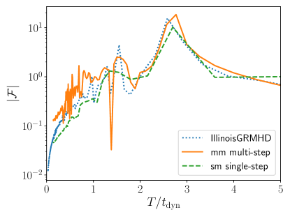
A Fourier transform of the fractional variation in central density further confirms qualitative agreement between IllinoisGRMHD and MANGA. Here we apply a Gaussian window function of the form to and take a Fourier power of , where . Changing the value of between 5 and 20 do not change our results significantly. In Figure 4, we plot the Fourier power, , as a function of the period, , in units of with arbitarily normalization. The crucial feature of this plot is that three runs agree on the position of the fundamental peak at , though it is less clear in the MANGA run with the static mesh and single timestep due to the shorter time series.
5 Conclusions and Future Work
We have reviewed the structure and implementation of a moving-mesh general relativistic hydrodynamics solver for static spacetimes in MANGA. Taking advantage that any flux-conservative equation can be solved on a moving, unstructured Voronoi mesh, we briefly describe the general algorithm to solve the GRHD equations. We then elaborate on a number of technical points including implementation of the van Leer method of second-order time integration, strategy for solving the Riemann problem across moving faces, transformation of primitives to/from conservatives variables, validation and correction of hydrodynamic variables, and mapping a spherically symmetric metric to a Voronoi grid.
We then apply our code to the analytic solution of a TOV star and show that our algorithm integrates the star stably as expected. In particular, we show that at high resolution ( mesh generating points inside the star) that the star is stable and the central density varies by at most 2% over 24 dynamical times. At lower resolution ( mesh generating points inside the star), the central density suffers a systematic drift toward lower density similar to that observed by Duez et al. (2005) on Eulerian (Cartesian) grids at low resolution with second order spatial reconstruction. Because our current MM method is limited to second-order reconstruction, we find that our results are consistent with that of Duez et al. (2005). Moreover, we also find that we can mitigate this effect in large part by going to higher resolution. Finally we demonstrate that when evolving the same star, but with its initial pressure depleted by 10%, we recover the same fundamental frequency of ensuing oscillations.
This paper is the first in a series that will describe the eventual implementation of a moving-mesh GRHD code on dynamical spacetimes. While the code can already be used to study flows around black holes and neutron stars, this is not our primary interest. Instead we aim to study the mergers of compact binaries with matter. Toward that end a number of future improvements are planned and will be described in future work. These are listed in order of priority:
-
1.
Incorporation of a full dynamical spacetime solver. While there are many applications of a moving-mesh GRHD solver in static spacetimes, our main interest is adapting our moving-mesh GRHD to NS-NS and NS-BH mergers. As such, we are incorporating the dynamical spacetime solver SENR/NRPy+ in MANGA. Here the major challenge is to couple the MANGA and SENR/NRPy+ codes, and get them to pass information between one another. We note that although SENR/NRPy+ is currently geared toward solving the binary BH problem (for which ), all source terms were recently added to Einstein’s equations within SENR/NRPy+ and validated666https://nbviewer.jupyter.org/github/zachetienne/nrpytutorial/blob/master/Tutorial-Start_to_Finish-BSSNCurvilinear-Neutron_Star-Hydro_without_Hydro.ipynb; download here: https://github.com/zachetienne/nrpytutorial for the case of a TOV star with a fixed stress-energy tensor but an evolving spacetime metric (the so-called “hydro without hydro” test of numerical relativity; Baumgarte et al. 1999).
-
2.
Implementation of piecewise-polytropic and tabulated equations of state. As part of our strategy to create realistic simulations of NS-NS and NS-BH mergers, we plan to implement realistic equations of state into MANGA with the GRHD solver. In this regard, we plan to both implement piecewise-polytropic and tabulated equations of state in MANGA. In fact, a nuclear equation of state has already been implemented (Schneider et al., 2017) in the Newtonian version of MANGA. The framework for implementation of generic equations of state is general and can be used (in the Newtonian case) for both the moving-mesh solver and the SPH solver (if required) of MANGA without modification. Here we plan to modify the framework to support the GRHD solver.
-
3.
Implementation of GRMHD. Magnetic fields play an important dynamical role in compact binary mergers with matter. Toward that end, we plan on implementing GRMHD in MANGA. To do this, we will need to modify the equation of hydrodynamics to include magnetic fields and include an evolution equation for the magnetic field. In moving, unstructured meshes, two different schemes have emerged for evolving the magnetic field while maintaining the divergence-free condition, , where is the magnetic field. These schemes are the divergence cleaning/diffusion methods, e.g., Dedner scheme (Dedner et al., 2002; Pakmor et al., 2011) and vector potential methods (Mocz et al., 2016). We have implemented an MHD scheme in MANGA based on the vector potential scheme of Mocz et al. (2016) and plan to adapt the scheme to the general relativistic case. As this method is similar to the currently implemented method in IllinoisGRMHD, we do not anticipate major technical challenges.
-
4.
Implementation of neutrino physics/radiation. Neutrinos affect the outflows and eventual r-process yields of NS-NS and NS-BH mergers, and can act as energizers of the outflows as well as changing the of the resulting outflowing material to change both the total mass of the outflow and its composition. To capture this physics, we plan to adapt our recent time-dependent radiative transfer algorithm (Chang et al., 2020) to include neutrino radiation. In particular, if we ignore metric effects on the radiation, e.g., straight-line propagation, the adaption of our current radiation methods would require the expansion from one photon species to the number of neutrino species and the addition of an evolution equation and source terms for the electron fraction (see for instance Müller et al., 2010; Skinner et al., 2019).
Acknowledgments
We acknowledge Charles Gammie, Andrew MacFadyen, Philipp Moesta, Kenta Hotokezaka, and Chris White for useful discussions. We thank Paul Duffell and Francois Foucart for crucial insights on the computation of the Riemann flux on unstructured grids. We also thank Scott Noble for providing a thread-safe version of his conservative-to-primitive solver. We thank the anonymous reviewer for helpful comments and criticisms. PC is supported by the NASA ATP program through NASA grant NNH17ZDA001N-ATP. PC acknowledges the support and hospitality of the Center for Computational Astrophysics at the Flatiron Institute where much of this work was carried out. ZBE gratefully acknowledges the NSF for financial support from awards OIA-1458952 and PHY-1806596; and NASA for financial support from awards ISFM-80NSSC18K0538 and TCAN-80NSSC18K1488. The authors acknowledge the Texas Advanced Computing Center (TACC) at The University of Texas at Austin for providing HPC resources that have contributed to the research results reported within this paper, http://www.tacc.utexas.edu. Computations were performed on the Niagara supercomputer at the SciNet HPC Consortium. SciNet is funded by: the Canada Foundation for Innovation; the Government of Ontario; Ontario Research Fund - Research Excellence; and the University of Toronto. IllinoisGRMHD simulations were completed on the Thorny Flat HPC System at West Virginia University (WVU), which was funded in part by the National Science Foundation (NSF) Major Research Instrumentation Program (MRI) Award #1726534, and WVU. We also use the yt software platform for the analysis of the data and generation of plots in this work (Turk et al., 2011). The Flatiron Institute is supported by the Simons Foundation.
References
- Aloy et al. (1999) Aloy M. A., Ibáñez J. M., Martí J. M., Müller E., 1999, ApJS, 122, 151
- Anderson et al. (2006) Anderson M., Hirschmann E., Liebling S. L., Neilsen D., 2006, Classical and Quantum Gravity, 23, 6503
- Baumgarte et al. (1999) Baumgarte T. W., Hughes S. A., Shapiro S. L., 1999, Phys. Rev., D60, 087501
- Burns et al. (2019) Burns K. J., Lecoanet D., Vasil G. M., Oishi J. S., Brown B. P., 2019, arXiv e-prints, p. arXiv:1903.12642
- Cerdá-Durán et al. (2008) Cerdá-Durán P., Font J. A., Antón L., Müller E., 2008, A&A, 492, 937
- Chang et al. (2017) Chang P., Wadsley J., Quinn T. R., 2017, MNRAS, 471, 3577
- Chang et al. (2020) Chang P., Davis S. W., Jiang Y., 2020, submitted to MNRAS
- Colella & Woodward (1984) Colella P., Woodward P. R., 1984, Journal of Computational Physics, 54, 174
- Dedner et al. (2002) Dedner A., Kemm F., Kröner D., Munz C. D., Schnitzer T., Wesenberg M., 2002, Journal of Computational Physics, 175, 645
- Dionysopoulou et al. (2013) Dionysopoulou K., Alic D., Palenzuela C., Rezzolla L., Giacomazzo B., 2013, Phys.Rev., D88, 044020
- Duez et al. (2005) Duez M. D., Liu Y. T., Shapiro S. L., Stephens B. C., 2005, Phys. Rev. D, 72, 024028:1
- Duez et al. (2008) Duez M. D., Foucart F., Kidder L. E., Pfeiffer H. P., Scheel M. A., Teukolsky S. A., 2008, Phys. Rev. D, 78, 104015
- Duffell (2016) Duffell P. C., 2016, ApJS, 226, 2
- Duffell & MacFadyen (2011) Duffell P. C., MacFadyen A. I., 2011, ApJS, 197, 15
- Etienne et al. (2015) Etienne Z. B., Paschalidis V., Haas R., Mösta P., Shapiro S. L., 2015, Classical and Quantum Gravity, 32, 175009:1
- Gaburov et al. (2012) Gaburov E., Johansen A., Levin Y., 2012, ApJ, 758, 103
- Giacomazzo & Rezzolla (2007) Giacomazzo B., Rezzolla L., 2007, Classical and Quantum Gravity, 24, S235
- Harten et al. (1983) Harten A., Lax P. D., van Leer B. J., 1983, SIAM Rev., 25, 35
- Hopkins (2015) Hopkins P. F., 2015, MNRAS, 450, 53
- Kidder et al. (2017) Kidder L. E., et al., 2017, Journal of Computational Physics, 335, 84
- Lamberts et al. (2013) Lamberts A., Fromang S., Dubus G., Teyssier R., 2013, A&A, 560, A79
- Lecoanet et al. (2016) Lecoanet D., et al., 2016, MNRAS, 455, 4274
- Loken et al. (2010) Loken C., et al., 2010, Journal of Physics: Conference Series, 256, 012026
- Mignone & Bodo (2005) Mignone A., Bodo G., 2005, MNRAS, 364, 126
- Mocz et al. (2014) Mocz P., Vogelsberger M., Hernquist L., 2014, MNRAS, 442, 43
- Mocz et al. (2015) Mocz P., Vogelsberger M., Pakmor R., Genel S., Springel V., Hernquist L., 2015, MNRAS, 452, 3853
- Mocz et al. (2016) Mocz P., Pakmor R., Springel V., Vogelsberger M., Marinacci F., Hernquist L., 2016, MNRAS, 463, 477
- Mösta et al. (2014) Mösta P., et al., 2014, Classical and Quantum Gravity, 31, 015005
- Müller et al. (2010) Müller B., Janka H.-T., Dimmelmeier H., 2010, ApJS, 189, 104
- Noble et al. (2006) Noble S. C., Gammie C. F., McKinney J. C., Del Zanna L., 2006, ApJ, 641, 626
- O’Connor & Ott (2010) O’Connor E., Ott C. D., 2010, Classical and Quantum Gravity, 27, 114103
- Oechslin et al. (2002) Oechslin R., Rosswog S., Thielemann F.-K., 2002, Phys. Rev. D, 65, 103005
- Ohlmann et al. (2016) Ohlmann S. T., Röpke F. K., Pakmor R., Springel V., 2016, ApJ, 816, L9
- Oppenheimer & Volkoff (1939) Oppenheimer J. R., Volkoff G. M., 1939, Physical Review, 55, 374
- Pakmor et al. (2011) Pakmor R., Bauer A., Springel V., 2011, MNRAS, 418, 1392
- Pakmor et al. (2016a) Pakmor R., Springel V., Bauer A., Mocz P., Munoz D. J., Ohlmann S. T., Schaal K., Zhu C., 2016a, MNRAS, 455, 1134
- Pakmor et al. (2016b) Pakmor R., Pfrommer C., Simpson C. M., Kannan R., Springel V., 2016b, MNRAS, 462, 2603
- Palenzuela (2013) Palenzuela C., 2013, MNRAS, 431, 1853
- Paxton et al. (2011) Paxton B., Bildsten L., Dotter A., Herwig F., Lesaffre P., Timmes F., 2011, ApJS, 192, 3
- Paxton et al. (2013) Paxton B., et al., 2013, ApJS, 208, 4
- Paxton et al. (2015) Paxton B., et al., 2015, ApJS, 220, 15
- Pfrommer et al. (2017) Pfrommer C., Pakmor R., Schaal K., Simpson C. M., Springel V., 2017, MNRAS, 465, 4500
- Ponce et al. (2019) Ponce M., et al., 2019, in Proceedings of the Practice and Experience in Advanced Research Computing on Rise of the Machines (Learning). PEARC ’19. Association for Computing Machinery, New York, NY, USA, doi:10.1145/3332186.3332195, https://doi.org/10.1145/3332186.3332195
- Prust (2020) Prust L., 2020, submitted to MNRAS
- Prust & Chang (2019) Prust L. J., Chang P., 2019, MNRAS, 486, 5809
- Radice et al. (2014) Radice D., Rezzolla L., Galeazzi F., 2014, Classical and Quantum Gravity, 31, 075012
- Ruchlin et al. (2018) Ruchlin I., Etienne Z. B., Baumgarte T. W., 2018, Phys. Rev. D, 97, 064036
- Ryan & MacFadyen (2017) Ryan G., MacFadyen A., 2017, ApJ, 835, 199
- Schneider et al. (2017) Schneider A. S., Roberts L. F., Ott C. D., 2017, Phys. Rev. C, 96, 065802
- Skinner et al. (2019) Skinner M. A., Dolence J. C., Burrows A., Radice D., Vartanyan D., 2019, ApJS, 241, 7
- Springel (2010) Springel V., 2010, MNRAS, 401, 791
- Timmes & Swesty (2000) Timmes F. X., Swesty F. D., 2000, ApJS, 126, 501
- Tolman (1934) Tolman R. C., 1934, Relativity, Thermodynamics, and Cosmology
- Toro (2009) Toro E., 2009, Riemann Solvers and Numerical Methods for Fluid Dynamics: A Practical Introduction. Springer Berlin Heidelberg
- Turk et al. (2011) Turk M. J., Smith B. D., Oishi J. S., Skory S., Skillman S. W., Abel T., Norman M. L., 2011, The Astrophysical Journal Supplement Series, 192, 9
- Vandenbroucke & De Rijcke (2016) Vandenbroucke B., De Rijcke S., 2016, Astronomy and Computing, 16, 109
- Vogelsberger et al. (2014) Vogelsberger M., et al., 2014, MNRAS, 444, 1518
- Weinberger et al. (2019) Weinberger R., Springel V., Pakmor R., 2019, arXiv e-prints, p. arXiv:1909.04667
- White et al. (2016) White C. J., Stone J. M., Gammie C. F., 2016, ApJS, 225, 22
- Yalinewich et al. (2015) Yalinewich A., Steinberg E., Sari R., 2015, ApJS, 216, 35
- Yamamoto et al. (2008) Yamamoto T., Shibata M., Taniguchi K., 2008, Phys. Rev. D, 78, 064054
- Zhu et al. (2015) Zhu C., Pakmor R., van Kerkwijk M. H., Chang P., 2015, ApJ, 806, L1