This paper was converted on www.awesomepapers.org from LaTeX by an anonymous user.
Want to know more? Visit the Converter page.

General condition of quantum teleportation
by one-dimensional quantum walks

Tomoki Yamagami Department of Information Physics and Computing, Graduate School of Information Science and Technology, The University of Tokyo, Tokyo, 113-8656, Japan.    Etsuo Segawa Graduate School of Environment and Information Sciences, Yokohama National University Yokohama, 240-8501, Japan.    Norio Konno Department of Applied Mathematics, Faculty of Engineering, Yokohama National University, Yokohama, 240-8501, Japan.

Abstract We extend the scheme of quantum teleportation by quantum walks introduced by Wang et al. (2017). First, we introduce the mathematical definition of the accomplishment of quantum teleportation by this extended scheme. Secondly, we show a useful necessary and sufficient condition that the quantum teleportation is accomplished rigorously. Our result classifies the parameters of the setting for the accomplishment of quantum teleportation.

1 Introduction

Quantum walk is considered as a quantum analogue of random walk. This model was first introduced in the context of quantum information theory such as Aharonov et al. [1] and Ambainis et al. [2]. Since then, quantum walk is treated as an interesting model in the field of mathematics and information theory [3, 4, 5, 6, 7] and expected of its application [8, 9]. Quantum walk is capable of universal quantum computation and able to be implemented by the physical system in various ways [10, 11, 12, 13], which is why the model is considered to be expectable one.

On the other hand, quantum teleportation is a communication protocol that transmits a quantum state from one place to another. It is first introduced by Bennett et al. [15] and regarded as not only a system for communication but also the basis of quantum computation [16].

Recently, the works on applications of quantum walks to quantum teleportation [17, 18, 19, 20] appear. In previous quantum teleportation systems, they had to produce prior entangled states and carried on transmission with it. However, by using quantum walks, the walk itself has a role of entanglement, which makes teleportation simpler. In the previous study [17], the concrete models of teleportation by quantum walks are shown, but the general condition where the scheme of teleportation succeeds is not shown. In this paper, we extend the scheme of quantum teleportation by quantum walks introduced by Wang et al. [17]. We introduce the mathematical definition of the accomplishment of quantum teleportation by this extended scheme. Then, we show a useful necessary and sufficient condition for it. Our result classifies the parameters of the setting for the accomplishment of the quantum teleportation including Wang et al.’s settings.

The rest of the paper is organized as follows. Section 2 gives the definition of our quantum walk model, and in Sect. 3 we give the scheme of teleportation by the quantum walk model. In Sect. 4, we present our main theorem of this paper and demonstrate some examples of the theorem. Furthermore, Sect. 5 is devoted to the proof of the result. Finally, we give a summary and discussion in Sect. 6.

2 Quantum Walks

Here, we introduce the quantum walks (QWs). First, we review a basic model of discrete QW and then introduce the QW applied to the scheme of quantum teleportation.

2.1 The One-Coin Quantum Walks on One-Dimensional Lattice

The one-dimensional quantum walk with one coin is defined in a compound Hilbert space of the position Hilbert space P=span{|x|x}\mathcal{H}_{\rm P}={\rm span}\{\ket{x}|x\in\mathbb{Z}\} and the coin Hilbert space C=span{|R,|L}\mathcal{H}_{\rm C}={\rm span}\{\ket{R},\,\ket{L}\} with

|R=[10],|L=[01].\displaystyle\ket{R}=\left[\begin{array}[]{c}1\\ 0\end{array}\right],\quad\ket{L}=\left[\begin{array}[]{c}0\\ 1\end{array}\right]. (5)

Note that C\mathcal{H_{\rm C}} is equivalent to 2\mathbb{C}^{2}. Then, the whole system is described by =PC\mathcal{H}=\mathcal{H}_{\rm P}\otimes\mathcal{H}_{\rm C}.

Now, we define one-step time evolution of the quantum walk as W=S^C^W=\hat{S}\cdot\hat{C}, where S^\hat{S} is a shift operator described by

S^=S|RR|+S1|LL|\displaystyle\hat{S}=S\otimes\ket{R}\bra{R}+S^{-1}\otimes\ket{L}\bra{L}

with

S=x|x+1x|,\displaystyle S=\sum_{x\in\mathbb{Z}}\ket{x+1}\bra{x},

and C^\hat{C} is a coin operator defined by

C^=I2C,\displaystyle\hat{C}=I_{2}\otimes C,

with

I2=[ 1 0 0 1],CU(2).\displaystyle I_{2}=\left[\begin{array}[]{cc}\,1&\,0\\ \,0&\,1\end{array}\right],\quad C\in{\rm U}(2). (8)

Here, U(nn) is the set of n×nn\times n unitary matrices.

2.2 mm-Coin Quantum Walks on One-Dimensional Lattice

To implement schemes of quantum teleportation based on quantum walks, we need to define quantum walks with many coins, which are determined on the whole system =PCm\mathcal{H}=\mathcal{H_{\rm P}}\otimes\mathcal{H_{\rm C}}^{\otimes m} with mnm\geq n (the previous case was one coin QW).

Now, we define one-step time evolution of the mm-coin quantum walk at time nn as Wn=S^nC^nW_{n}=\hat{S}_{n}\cdot\hat{C}_{n}, where S^n\hat{S}_{n} is a shift operator described by

S^n\displaystyle\hat{S}_{n} =\displaystyle= S(I2I2|RR|nI2I2)\displaystyle S\otimes\left(I_{2}\otimes\cdots\otimes I_{2}\otimes\overbrace{\ket{R}\bra{R}}^{n}\otimes I_{2}\otimes\cdots\otimes I_{2}\right)
+S1(I2I2|LL|nI2I2),\displaystyle+S^{-1}\otimes\left(I_{2}\otimes\cdots\otimes I_{2}\otimes\overbrace{\ket{L}\bra{L}}^{n}\otimes I_{2}\otimes\cdots\otimes I_{2}\right),

and C^n\hat{C}_{n} is the coin operator described by

C^n=I(I2I2CnnI2I2).\displaystyle\hat{C}_{n}=I_{\infty}\otimes\left(I_{2}\otimes\cdots\otimes I_{2}\otimes\overbrace{C_{n}}^{n}\otimes I_{2}\otimes\cdots\otimes I_{2}\right).

Here, “n\overbrace{}^{n}” means that the matrix corresponds to nnth C\mathcal{H_{\rm C}} and CnU(2)C_{n}\in{\rm U}(2).

Moreover, we put

Pn=|LL|Cn,Qn=|RR|Cn.\displaystyle P_{n}=\ket{L}\bra{L}C_{n},\quad Q_{n}=\ket{R}\bra{R}C_{n}.

We should note that Cn=Pn+QnC_{n}=P_{n}+Q_{n}. Then, a quantum walker at time nn moves one unit to the left with the weight

I2I2PnnI2I2,\displaystyle I_{2}\otimes\cdots\otimes I_{2}\otimes\overbrace{P_{n}}^{n}\otimes I_{2}\otimes\cdots\otimes I_{2},

or to the right with weight

I2I2QnnI2I2.\displaystyle I_{2}\otimes\cdots\otimes I_{2}\otimes\overbrace{Q_{n}}^{n}\otimes I_{2}\otimes\cdots\otimes I_{2}.

In other words, for nn\in\mathbb{Z}_{\geq} and |Ψn\ket{\varPsi_{n}}, the state of the system at time nn, the relationship between the states |Ψn\ket{\varPsi_{n}} and |Ψn+1\ket{\varPsi_{n+1}} is described as

|Ψn+1=Wn+1|Ψn.\displaystyle\ket{\varPsi_{n+1}}=W_{n+1}\ket{\varPsi_{n}}.

3 Schemes of Teleportation

Let us set PC(A)\mathcal{H_{\rm P}}\otimes\mathcal{H_{\rm C}^{\rm(\rm A)}} and C(B)\mathcal{H_{\rm C}^{\rm(\rm B)}} as the Alice and Bob’s spaces, respectively after the fashion of the proposed idea by [17]. Here, C(A)\mathcal{H_{\rm C}^{\rm(\rm A)}}, C(B)2\mathcal{H_{\rm C}^{\rm(\rm B)}}\cong\mathbb{C}^{2}. In this section, we consider quantum teleportation described in Figure 1. Now, the sender Alice wants to send |ϕC(A)(2)\ket{\phi}\in\mathcal{H_{\rm C}^{\rm(\rm A)}}(\cong\mathbb{C}^{2}) with ϕ=1\|\phi\|=1 to the receiver Bob. We call |ϕ\ket{\phi} the target state.

The space of this quantum teleportation is denoted by =PC(A)C(B)\mathcal{H}=\mathcal{H_{\rm P}}\otimes\mathcal{H_{\rm C}^{\rm(A)}}\otimes\mathcal{H_{\rm C}^{\rm(B)}}. We set the initial state as

|Ψ0=|0|ϕ|ψ.\displaystyle\ket{\varPsi_{0}}=\ket{0}\otimes\ket{\phi}\otimes\ket{\psi}\in\mathcal{H}.

Here, |ψ\ket{\psi} satisfies ψ=1\|\psi\|=1. In the framework of quantum walk, the total state space of quantum teleportation is isomorphic to a two-coin quantum walk whose position Hilbert space is P\mathcal{H_{\rm P}} and whose coin Hilbert space is C(A)C(B)\mathcal{H_{\rm C}^{\rm(A)}}\otimes\mathcal{H_{\rm C}^{\rm(B)}}. On the other hand, from the point of view of quantum teleportation, Alice has two initial states |0|ϕPC(A)\ket{0}\otimes\ket{\phi}\in\mathcal{H_{\rm P}}\otimes\mathcal{H_{\rm C}^{\rm(A)}} and Bob has an initial state |ψC(B)\ket{\psi}\in\mathcal{H_{\rm C}^{\rm(B)}}, and the goal of the teleportation is that Bob obtains the state |ϕ\ket{\phi} as the element of C(B)\mathcal{H_{\rm C}^{\rm(B)}}.

Refer to caption
Figure 1: Circuit diagram of quantum teleportation by 2-coin quantum walks

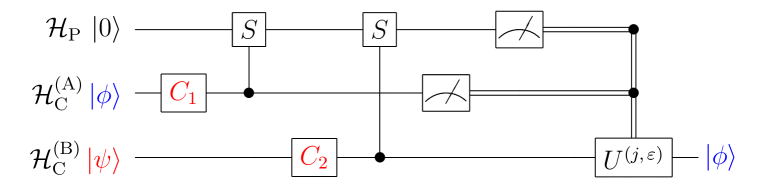
Then, we provide three stages: (1) time evolution, (2) measurement and (3) transformation.

3.1 Time Evolution by QW

In the first stage, we take 2 steps of QWs with two coins; we describe the time evolution operator at the first and second steps W1W_{1}, W2W_{2} as

W1=S1^C1^=(S|RR|I2+S1|LL|I2)(IC1I2),\displaystyle W_{1}=\hat{S_{1}}\cdot\hat{C_{1}}=(S\otimes\ket{R}\bra{R}\otimes I_{2}+S^{-1}\otimes\ket{L}\bra{L}\otimes I_{2})(I_{\infty}\otimes C_{1}\otimes I_{2}),
W2=S2^C2^=(SI2|RR|+S1I2|LL|)(II2C2),\displaystyle W_{2}=\hat{S_{2}}\cdot\hat{C_{2}}=(S\otimes I_{2}\otimes\ket{R}\bra{R}+S^{-1}\otimes I_{2}\otimes\ket{L}\bra{L})(I_{\infty}\otimes I_{2}\otimes C_{2}),

respectively. Suppose |Ψn\ket{\varPsi_{n}}\in\mathcal{H} (n=0,1,2)(n=0,1,2) is the state after the nn-th time evolution of the QW, and we regard the initial state of |Ψ0\ket{\varPsi_{0}} of the quantum teleportation as the initial state of the QW. We run this QW for two steps, that is,

|Ψ0W1|Ψ1W2|Ψ2.\displaystyle\ket{\varPsi_{0}}\stackrel{{\scriptstyle W_{1}}}{{\longmapsto}}\ket{\varPsi_{1}}\stackrel{{\scriptstyle W_{2}}}{{\longmapsto}}\ket{\varPsi_{2}}.

3.2 Measurement

In the second stage, to carry out the measurement on the Alice’s state, we introduce the observables denoted by self-adjoint operators M1M_{1} and M2M_{2} on C(A)\mathcal{H_{\rm C}^{\rm(A)}} and P\mathcal{H_{\rm P}}, respectively, as follows:

M1\displaystyle M_{1} =\displaystyle= (+1)|ηRηR|+(1)|ηLηL|,\displaystyle(+1)\ket{\eta_{R}}\bra{\eta_{R}}+(-1)\ket{\eta_{L}}\bra{\eta_{L}},
M2\displaystyle M_{2} =\displaystyle= jj2|ξjξj|,\displaystyle\sum_{j\in\mathbb{Z}}\frac{\,j\,}{2}\ket{\xi_{j}}\bra{\xi_{j}},

where |ηε=H1|ε(ε{R,L})\ket{\eta_{\varepsilon}}=H_{1}\ket{\varepsilon}\,(\varepsilon\in\{R,\,L\}), and |ξj=H2|j(j)\ket{\xi_{j}}=H_{2}\ket{j}\,(j\in\mathbb{Z}). Here, H1H_{1} and H2H_{2} are unitary operators on C(A)(2)\mathcal{H_{\rm C}^{\rm(A)}}(\cong\mathbb{C}^{2}) and P(2())\mathcal{H_{\rm P}}(\cong\ell^{2}({\mathbb{Z}})), respectively. Especially, H2H_{2} is described as follow:

H2[α22α20α2(2)α02α00α0(2)Oα(2)2α(2)0α(2)(2)OI]=[H~2OOI],\displaystyle H_{2}\simeq\left[\begin{array}[]{ccc|ccc}\alpha_{22}&\alpha_{20}&\alpha_{2{(-2)}}&&&\\ \alpha_{02}&\alpha_{00}&\alpha_{0{(-2)}}&\lx@intercol\hfil\raisebox{-3.0pt}[0.0pt][0.0pt]{\LARGE$\,\,\,O$}\hfil\lx@intercol&\\ \alpha_{{(-2)}2}&\alpha_{{(-2)}0}&\alpha_{{(-2)}{(-2)}}&&&\\ \hline\cr&&&&&\\ \lx@intercol\hfil\raisebox{3.0pt}[0.0pt][0.0pt]{\LARGE$\,\,\,\,\,\,O$}\hfil\lx@intercol&&\lx@intercol\hfil\raisebox{3.0pt}[0.0pt][0.0pt]{\LARGE$\,\,\,I$}\hfil\lx@intercol&\end{array}\right]=\left[\begin{array}[]{ccc|ccc}&&&&&\\ \lx@intercol\hfil\raisebox{3.0pt}[0.0pt][0.0pt]{\LARGE$\,\,\tilde{H}_{2}$}\hfil\lx@intercol&&\lx@intercol\hfil\raisebox{3.0pt}[0.0pt][0.0pt]{\LARGE$\,\,O$}\hfil\lx@intercol&\\ \hline\cr&&&&&\\ \lx@intercol\hfil\raisebox{3.0pt}[0.0pt][0.0pt]{\LARGE$\,\,O$}\hfil\lx@intercol&&\lx@intercol\hfil\raisebox{3.0pt}[0.0pt][0.0pt]{\LARGE$\,\,I$}\hfil\lx@intercol&\end{array}\right], (18)

where

H~2=[α22α20α2(2)α02α00α0(2)α(2)2α(2)0α(2)(2)].\displaystyle\tilde{H}_{2}=\left[\begin{array}[]{ccc}\alpha_{22}&\alpha_{20}&\alpha_{2{(-2)}}\\ \alpha_{02}&\alpha_{00}&\alpha_{0{(-2)}}\\ \alpha_{{(-2)}2}&\alpha_{{(-2)}0}&\alpha_{{(-2)}{(-2)}}\end{array}\right]. (22)

The computational basis of H2H_{2} in RHS is {|2,|0,|2,}\{\ket{2},\,\ket{0},\,\ket{-2},\,\ldots\} by this order. The observed values of the observable M1M_{1} are ε{±1}\varepsilon\in\{\pm 1\} after the description of [17], but in this paper, we describe the observed values of M1M_{1} by R,LR,L by the bijection map

R+1 and L1.R\leftrightarrow+1\text{ and }L\leftrightarrow-1.

In the same way, we describe the observed values of M2M_{2} as {2,0,2}\{-2,0,2\} by the bijection map

2kk(k=1,0,1).2k\leftrightarrow k\;(k=-1,0,1).

Furthermore, we extend the domains of operators M1M_{1} and M2M_{2} to the whole system \mathcal{H} by putting M1(s)M_{1}^{\rm(s)} and M2(s)M_{2}^{\rm(s)} as follows:

M1(s)\displaystyle M_{1}^{\rm(s)} :=IM1IC(B),\displaystyle:=I_{\infty}\otimes M_{1}\otimes I_{\mathcal{H_{\rm C}^{\rm(B)}}},
M2(s)\displaystyle M_{2}^{\rm(s)} :=M2IC(A)IC(B).\displaystyle:=M_{2}\otimes I_{\mathcal{H_{\rm C}^{\rm(A)}}}\otimes I_{\mathcal{H_{\rm C}^{\rm(B)}}}.

This means that Alice carries out projection measurements on C(A)\mathcal{H_{\rm C}^{\rm(A)}} and P\mathcal{H_{\rm P}} with the eigenvectors 1={|ηε|ε{R,L}}\mathcal{B}_{1}=\{\ket{\eta_{\varepsilon}}|\varepsilon\in\{R,\,L\}\} of M1M_{1} and 2={|ξj|j}\mathcal{B}_{2}=\{\ket{\xi_{j}}|j\in\mathbb{Z}\} of M2M_{2}, respectively. If Alice gets the observed values ε\varepsilon by M1M_{1} and jj by M2M_{2}, respectively, then the states collapse to |ηεC(A)\ket{\eta_{\varepsilon}}\in\mathcal{H}_{C}^{(A)} and |ξjP\ket{\xi_{j}}\in\mathcal{H}_{P}, respectively.

Through the measurements, if the state of C(A)\mathcal{H_{\rm C}^{\rm(A)}} collapses to |ηε1\ket{\eta_{\varepsilon}}\in\mathcal{B}_{1} by M1M_{1} and the state of P\mathcal{H_{\rm P}} collapses to |ξj2\ket{\xi_{j}}\in\mathcal{B}_{2} by M2M_{2}, the degenerate state on the whole state is denoted by |Ψ(j,ε)\ket{\varPsi_{*}^{(j,\,\varepsilon)}}\in\mathcal{H}. So, the state |Ψ(j,ε)\ket{\varPsi_{*}^{(j,\,\varepsilon)}} can be described explicitly as follows. The proof is given in Sect. 5.

Proposition 1.

The state |Ψ(j,ε)\ket{\varPsi_{*}^{(j,\,\varepsilon)}} can be described as

|Ψ(j,ε)=|ξj|ηε|Φ(j,ε),\displaystyle\ket{\varPsi_{*}^{(j,\,\varepsilon)}}=\ket{\xi_{j}}\otimes\ket{\eta_{\varepsilon}}\otimes\ket{\varPhi_{*}^{(j,\,\varepsilon)}}, (23)

where |Φ(j,ε)=V(j,ε)|ϕ\ket{\varPhi_{*}^{(j,\,\varepsilon)}}=V^{(j,\,\varepsilon)}\ket{\phi} and V(j,ε)V^{(j,\,\varepsilon)} is a linear map on C(B)\mathcal{H_{\rm C}^{\rm(B)}} (See (37) for the detailed expression for V(j,ε)V^{(j,\,\varepsilon)}).

Then, our problem is converted to finding a practical necessary and sufficient condition for the unitarity of V(j,ε)V^{(j,\,\varepsilon)}.

3.3 Transformation

In the final stage, Bob should convert his state |Φ(j,ε)C(B)\ket{\varPhi_{*}^{(j,\,\varepsilon)}}\in\mathcal{H_{\rm C}^{\rm(B)}} to the state |ϕ\ket{\phi}. After the measurements, Alice sends the outcomes ε{L,R}\varepsilon\in\{L,R\} and j{2,0,2}j\in\{-2,0,2\} to Bob. Then, Bob acts a unitary operator U(j,ε)U^{(j,\,\varepsilon)} on C(B)\mathcal{H_{\rm C}^{\rm(B)}} to |Φ(j,ε)\ket{\varPhi_{*}^{(j,\,\varepsilon)}}, depending on a pair of observed results (j,ε)(j,\,\varepsilon). Finally, Bob obtains a state |Φ:=U(j,ε)|Φ(j,ε)C(B)\ket{\varPhi}:=U^{(j,\,\varepsilon)}\ket{\varPhi_{*}^{(j,\,\varepsilon)}}\in\mathcal{H_{\rm C}^{\rm(B)}}. If |Φ=|ϕ\ket{\varPhi}=\ket{\phi}, we can regard that the teleportation is “accomplished” (we define this clearly below).

3.4 A mathematical formulation of schemes of teleportation

In the above subsections, we introduced the notion of quantum teleportation driven by quantum walk. As we have seen, the factors to determine the scheme of this teleportation are Bob’s initial state |ψ\ket{\psi}, the coin operators C1C_{1} and C2C_{2}, and the measurement operator H1H_{1} and H2H_{2}. Then, for convenience, we define the set of them as the parameter of the teleportation as follows:

Definition 2.

We call

𝑻=(|ψ;C1,C2;H1,H2)2×U(2)×U(2)×U(2)×U()\displaystyle\mbox{\boldmath$T$}=(\ket{\psi};\,C_{1},\,C_{2};\,H_{1},\,H_{2})\in{\rm\mathbb{C}^{2}\times U(2)\times U(2)\times U(2)\times U(\infty)}

a quantum walk measurement procedure.

Definition 3.

Let |ΦC(B)\ket{\varPhi}\in\mathcal{H_{\rm C}^{\rm(B)}} be a Bob’s final state of a quantum walk measurement procedure 𝑻T and |ϕC(A)\ket{\phi}\in\mathcal{H_{\rm C}^{\rm(A)}} be the target state. If this quantum walk measurement procedure 𝑻T satisfies |Φ=|ϕ\ket{\varPhi}=\ket{\phi} for any observed value (j,ε){2,0,2}×{L,R}(j,\,\varepsilon)\in\{-2,0,2\}\times\{L,R\} by Alice, we say that the quantum teleportation is accomplished by TT.

Definition 4.

We define 𝒯2×U(2)×U(2)×U(2)×U()\mathcal{T}\subset{\rm\mathbb{C}^{2}\times U(2)\times U(2)\times U(2)\times U(\infty)} by

𝒯:={𝑻=(|ψ;C1,C2;H1,H2)|𝑻 accomplishes  the  quantum  teleportation.}\displaystyle\mathcal{T}:=\left\{\mbox{\boldmath$T$}=(\ket{\psi};\,C_{1},\,C_{2};\,H_{1},\,H_{2})\,|\,\scalebox{0.8}[1.0]{\rm{\mbox{\boldmath$T$}}\, accomplishes\, the\, quantum\, teleportation.}\right\}

and call 𝒯\mathcal{T} the class of quantum teleportation driven by 2-coin quantum walks.

The main purpose of this paper is to determine explicitly the class 𝒯\mathcal{T}.

4 Our result

In this section, we present our main result on the quantum teleportation by quantum walks.

4.1 Main Theorem

Theorem 5.

Quantum walk measurement procedure 𝑻=(|ψ;C1,C2;H1,H2)\mbox{\boldmath$T$}=(\ket{\psi};\,C_{1},\,C_{2};\,H_{1},\,H_{2}) accomplishes the quantum teleportation, i.e., 𝑻𝒯\mbox{\boldmath$T$}\in\mathcal{T} iff 𝑻T satisfies the following three conditions simultaneously:

  1. (I)

    [Condition for H1H_{1}] |R|H1|R|=|R|H1|L||\braket{R}{H_{1}}{R}|=|{\braket{R}{H_{1}}{L}}|.

  2. (II)

    [Condition for C2C_{2} and ψ\psi ] |R|C2|ψ|=|L|C2|ψ|=12\left|\left\langle R|C_{2}|\psi\right\rangle\right|=\left|\left\langle L|C_{2}|\psi\right\rangle\right|=\displaystyle\frac{1}{\sqrt{2}}.

  3. (III)

    [Condition for H2H_{2}] 𝑻T satisfies one of the following two conditions at least:

    1. (i)

      Let 𝑯H be the set of three-dimensional unitary matrices defined by

      𝑯={[pr000tqs0],[p0r0t0q0s],[0prt000qs]U(3):|p|=|q|}\mbox{\boldmath$H$}=\left\{\begin{bmatrix}p&r&0\\ 0&0&t\\ q&s&0\end{bmatrix},\;\begin{bmatrix}p&0&r\\ 0&t&0\\ q&0&s\end{bmatrix},\;\begin{bmatrix}0&p&r\\ t&0&0\\ 0&q&s\end{bmatrix}\in{\rm U}(3)\;:\;|p|=|q|\right\}

      Then, H2=H~2IH_{2}=\tilde{H}_{2}\oplus I_{\infty} with H~2𝑯\tilde{H}_{2}\in\mbox{\boldmath$H$}.

    2. (ii)

      for all k{0,±2}k\in\{0,\,\pm 2\},

      |(H2)2k|=|(H2)(2)k|\displaystyle|(H_{2})_{2k}|=|(H_{2})_{{(-2)}k}|

      and

      arg(H2)2k+arg(H2)(2)k2arg(H2)0k(2+1)π.\displaystyle{\rm arg}(H_{2})_{2k}+{\rm arg}(H_{2})_{{(-2)}k}-2{\rm arg}(H_{2})_{0k}\in(2\mathbb{Z}+1)\pi.

    Here, (H2)jk=j|H2|k(H_{2})_{jk}=\braket{j}{H_{2}}{k}.

Moreover, in any case, the transformation U(j,ε)U^{(j,\,\varepsilon)} by Bob depending on observed results (j,ε)(j,\,\varepsilon) is unitary described as

U(j,ε)=1V(j,ε)|ϕ(V(j,ε))1,\displaystyle U^{(j,\,\varepsilon)}=\frac{1}{\|V^{(j,\,\varepsilon)}\ket{\phi}\|}\left(V^{(j,\,\varepsilon)}\right)^{-1},

where

V(j,ε)=[ηε|(α2j¯Q1+α0j¯P1)βRηε|(α0j¯Q1+α(2)j¯P1)βL],\displaystyle V^{(j,\,\varepsilon)}=\left[\begin{array}[]{cc}\bra{\eta_{\varepsilon}}(\overline{\alpha_{2j}}Q_{1}+\overline{\alpha_{0j}}P_{1})\beta_{R}\\ \bra{\eta_{\varepsilon}}(\overline{\alpha_{0j}}Q_{1}+\overline{\alpha_{(-2)j}}P_{1})\beta_{L}\end{array}\right], (26)

regardless of |ϕ\ket{\phi}. Here αjk=(H2)jk\alpha_{jk}=(H_{2})_{jk} and βL=L|C2|ψ\beta_{L}=\bra{L}C_{2}\ket{\psi}, βR=R|C2|ψ\beta_{R}=\bra{R}C_{2}\ket{\psi}.

Remark 6.

This theorem implies that accomplishment of the quantum teleportation is independent of C1C_{1}. Moreover, the theorem does not depend on C2C_{2} and |ψ\ket{\psi}, for each one, but “C2|ψC_{2}\ket{\psi}.” After all, the accomplishment of quantum teleportation is determined only by three factors, that is, H1H_{1}, H2H_{2}, and |ψ=C2|ψ\ket{\psi^{\prime}}=C_{2}\ket{\psi}; this is a generalization of the statement of [17].

Remark 7.

The condition (II) means that the coin operator C2C_{2} must be unbiased. This claim agrees with Li et al. [19], in which it is the case of the number of qubit N=1N=1.

4.2 Examples and Demonstrations

In the following, we put H=12[1111]H=\displaystyle\frac{1}{\sqrt{2}}\left[\begin{array}[]{cc}1&1\\ 1&-1\end{array}\right].

  1. (1)

    We choose

    |ψ=|R,C1=I2,C2=H1=H,H~2HI.\displaystyle\ket{\psi}=\ket{R},\,\,C_{1}=I_{2},\,\,C_{2}=H_{1}=H,\,\,\tilde{H}_{2}\simeq H\oplus{I_{\infty}}.

    This case satisfies (III)-(i) and Wang et al.[17] has shown that in this case the quantum teleportation is accomplished. Bob’s state before measurement |Φ(j,ε)\ket{\varPhi^{(j,\,\varepsilon)}} and the operator U(j,ε)U^{(j,\,\varepsilon)} are as follows:

    (j,ε)|Φ(j,ε)U(j,ε)(2,R)|ϕI2(0,R)X|ϕX(2,R)Z|ϕZ(2,L)Z|ϕZ(0,L)XZ|ϕZX(2,L)|ϕI2\displaystyle\begin{array}[]{|c|c|c|}\hline\cr(j,\,\varepsilon)&\quad\quad\ket{\varPhi^{(j,\,\varepsilon)}}&\quad\quad U^{(j,\,\varepsilon)}\quad\quad\vrule width=0.0pt,height=13.0pt,depth=8.0pt\\ \hline\cr\hline\cr(2,\,R)&\ket{\phi}&I_{2}\vrule width=0.0pt,height=13.0pt,depth=8.0pt\\ \hline\cr(0,\,R)&X\ket{\phi}&X\vrule width=0.0pt,height=13.0pt,depth=8.0pt\\ \hline\cr(-2,\,R)&Z\ket{\phi}&Z\vrule width=0.0pt,height=13.0pt,depth=8.0pt\\ \hline\cr(2,\,L)&Z\ket{\phi}&Z\vrule width=0.0pt,height=13.0pt,depth=8.0pt\\ \hline\cr(0,\,L)&XZ\ket{\phi}&ZX\vrule width=0.0pt,height=13.0pt,depth=8.0pt\\ \hline\cr(-2,\,L)&\ket{\phi}&I_{2}\vrule width=0.0pt,height=13.0pt,depth=8.0pt\\ \hline\cr\end{array}
  2. (2)

    We choose

    |ψ=|R+|L2,C1=C2=I2,H1=H,H~2=13[e43πi1e23πi111e23πi1e43πi].\displaystyle\ket{\psi}=\frac{\ket{R}+\ket{L}}{\sqrt{2}},\,\,C_{1}=C_{2}=I_{2},\,H_{1}=H,\,\,\tilde{H}_{2}=\displaystyle\frac{1}{\sqrt{3}}\left[\begin{array}[]{ccc}-e^{\frac{4}{3}\pi i}&-1&-e^{\frac{2}{3}\pi i}\\ 1&1&1\\ e^{\frac{2}{3}\pi i}&1&e^{\frac{4}{3}\pi i}\end{array}\right]. (30)

    This case satisfies (III)-(ii). Bob’s state before measurement |Φ(j,ε)\ket{\varPhi^{(j,\,\varepsilon)}} and the operator U(j,ε)U^{(j,\,\varepsilon)} are as follows:

    (j,ε)|Φ(j,ε)U(j,ε)(2,R)12[e23πi11e43πi]|ϕ12[e43πi11e23πi](0,R)12[1111]|ϕ12[1111](2,R)12[e43πi11e23πi]|ϕ12[e23πi11e43πi](2,L)12[e23πi11e43πi]|ϕ12[e43πi11e23πi](0,L)12[1111]|ϕ12[1111](2,L)12[e43πi11e23πi]|ϕ12[e23πi11e43πi]\displaystyle\begin{array}[]{|c|c|c|}\hline\cr(j,\,\varepsilon)&\ket{\varPhi^{(j,\,\varepsilon)}}&U^{(j,\,\varepsilon)}\vrule width=0.0pt,height=13.0pt,depth=8.0pt\\ \hline\cr\hline\cr(2,\,R)&\quad\displaystyle\frac{1}{\sqrt{2}}\left[\begin{array}[]{cc}e^{\frac{2}{3}\pi i}&1\\ 1&-e^{\frac{4}{3}\pi i}\end{array}\right]\ket{\phi}&\quad\displaystyle\frac{1}{\sqrt{2}}\left[\begin{array}[]{cc}e^{\frac{4}{3}\pi i}&1\\ 1&-e^{\frac{2}{3}\pi i}\end{array}\right]\quad\vrule width=0.0pt,height=20.0pt,depth=15.0pt\\ \hline\cr(0,\,R)&\displaystyle\frac{1}{\sqrt{2}}\left[\begin{array}[]{cc}1&1\\ 1&-1\end{array}\right]\ket{\phi}&\displaystyle\frac{1}{\sqrt{2}}\left[\begin{array}[]{cc}1&1\\ 1&-1\end{array}\right]\vrule width=0.0pt,height=20.0pt,depth=15.0pt\\ \hline\cr(-2,\,R)&\displaystyle\frac{1}{\sqrt{2}}\left[\begin{array}[]{cc}e^{\frac{4}{3}\pi i}&1\\ 1&-e^{\frac{2}{3}\pi i}\end{array}\right]\ket{\phi}&\displaystyle\frac{1}{\sqrt{2}}\left[\begin{array}[]{cc}e^{\frac{2}{3}\pi i}&1\\ 1&-e^{\frac{4}{3}\pi i}\end{array}\right]\vrule width=0.0pt,height=20.0pt,depth=15.0pt\\ \hline\cr(2,\,L)&\displaystyle\frac{1}{\sqrt{2}}\left[\begin{array}[]{cc}e^{\frac{2}{3}\pi i}&-1\\ 1&e^{\frac{4}{3}\pi i}\end{array}\right]\ket{\phi}&\displaystyle\frac{1}{\sqrt{2}}\left[\begin{array}[]{cc}e^{\frac{4}{3}\pi i}&1\\ -1&e^{\frac{2}{3}\pi i}\end{array}\right]\vrule width=0.0pt,height=20.0pt,depth=15.0pt\\ \hline\cr(0,\,L)&\displaystyle\frac{1}{\sqrt{2}}\left[\begin{array}[]{cc}1&-1\\ 1&1\end{array}\right]\ket{\phi}&\displaystyle\frac{1}{\sqrt{2}}\left[\begin{array}[]{cc}1&1\\ -1&1\end{array}\right]\vrule width=0.0pt,height=20.0pt,depth=15.0pt\\ \hline\cr(-2,\,L)&\displaystyle\frac{1}{\sqrt{2}}\left[\begin{array}[]{cc}e^{\frac{4}{3}\pi i}&-1\\ 1&e^{\frac{2}{3}\pi i}\end{array}\right]\ket{\phi}&\displaystyle\frac{1}{\sqrt{2}}\left[\begin{array}[]{cc}e^{\frac{2}{3}\pi i}&1\\ -1&e^{\frac{4}{3}\pi i}\end{array}\right]\vrule width=0.0pt,height=20.0pt,depth=15.0pt\\ \hline\cr\end{array}
  3. (3)

    We choose

    |ψ=|R+i|L2,C1=C2=I2,H1=H,H~2=[i/21/2i/21/201/2i/21/2i/2].\displaystyle\ket{\psi}=\frac{\ket{R}+i\ket{L}}{\sqrt{2}},\,\,C_{1}=C_{2}=I_{2},\,\,H_{1}=H,\,\,\tilde{H}_{2}=\left[\begin{array}[]{ccc}i/2&1/\sqrt{2}&-i/2\\ 1/\sqrt{2}&0&1/\sqrt{2}\\ i/2&-1/\sqrt{2}&-i/2\end{array}\right]. (34)

    This case is another example of (III)-(ii). Bob’s state before measurement |Φ(j,ε)\ket{\varPhi^{(j,\,\varepsilon)}} and the operator U(j,ε)U^{(j,\,\varepsilon)} are as follows:

    (j,ε)|Φ(j,ε)U(j,ε)(2,R)13[i22i1]|ϕ13[i2i21](0,R)[100i]|ϕ[100i](2,R)13[i22i1]|ϕ13[i2i21](2,L)13[i22i1]|ϕ13[i2i21](0,L)[100i]|ϕ[100i](2,L)13[i22i1]|ϕ13[i2i21]\displaystyle\begin{array}[]{|c|c|c|}\hline\cr(j,\,\varepsilon)&\ket{\varPhi^{(j,\,\varepsilon)}}&U^{(j,\,\varepsilon)}\vrule width=0.0pt,height=13.0pt,depth=8.0pt\\ \hline\cr\hline\cr(2,\,R)&\quad\displaystyle\frac{1}{\sqrt{3}}\left[\begin{array}[]{cc}i&\sqrt{2}\\ \sqrt{2}i&-1\end{array}\right]\ket{\phi}&\quad\displaystyle\frac{1}{\sqrt{3}}\left[\begin{array}[]{cc}-i&-\sqrt{2}i\\ \sqrt{2}&-1\end{array}\right]\quad\vrule width=0.0pt,height=20.0pt,depth=15.0pt\\ \hline\cr(0,\,R)&\left[\begin{array}[]{cc}-1&0\\ 0&i\end{array}\right]\ket{\phi}&\left[\begin{array}[]{cc}-1&0\\ 0&-i\end{array}\right]\vrule width=0.0pt,height=20.0pt,depth=15.0pt\\ \hline\cr(-2,\,R)&\displaystyle\frac{1}{\sqrt{3}}\left[\begin{array}[]{cc}-i&\sqrt{2}\\ \sqrt{2}i&1\end{array}\right]\ket{\phi}&\displaystyle\frac{1}{\sqrt{3}}\left[\begin{array}[]{cc}i&-\sqrt{2}i\\ \sqrt{2}&1\end{array}\right]\vrule width=0.0pt,height=20.0pt,depth=15.0pt\\ \hline\cr(2,\,L)&\displaystyle\frac{1}{\sqrt{3}}\left[\begin{array}[]{cc}i&-\sqrt{2}\\ \sqrt{2}i&1\end{array}\right]\ket{\phi}&\displaystyle\frac{1}{\sqrt{3}}\left[\begin{array}[]{cc}-i&-\sqrt{2}i\\ -\sqrt{2}&1\end{array}\right]\vrule width=0.0pt,height=20.0pt,depth=15.0pt\\ \hline\cr(0,\,L)&\left[\begin{array}[]{cc}-1&0\\ 0&-i\end{array}\right]\ket{\phi}&\left[\begin{array}[]{cc}-1&0\\ 0&i\end{array}\right]\vrule width=0.0pt,height=20.0pt,depth=15.0pt\\ \hline\cr(-2,\,L)&\displaystyle\frac{1}{\sqrt{3}}\left[\begin{array}[]{cc}-i&-\sqrt{2}\\ \sqrt{2}i&-1\end{array}\right]\ket{\phi}&\displaystyle\frac{1}{\sqrt{3}}\left[\begin{array}[]{cc}i&-\sqrt{2}i\\ -\sqrt{2}&-1\end{array}\right]\vrule width=0.0pt,height=20.0pt,depth=15.0pt\\ \hline\cr\end{array}

5 Proof of Main Theorem

5.1 Proof of Proposition 1

Proof.

At n=1n=1, |Ψ0\ket{\varPsi_{0}} evolves to

|Ψ1=W1|Ψ0=|1|Q1ϕ|ψ+|1|P1ϕ|ψ,\displaystyle\ket{\varPsi_{1}}=W_{1}\ket{\varPsi_{0}}=\ket{1}\otimes\ket{Q_{1}\phi}\otimes\ket{\psi}+\ket{-1}\otimes\ket{P_{1}\phi}\otimes\ket{\psi},

and at n=2n=2, |Ψ1\ket{\varPsi_{1}} evolves to

|Ψ2=W2|Ψ1=\displaystyle\ket{\varPsi_{2}}=W_{2}\ket{\varPsi_{1}}= |2|Q1ϕ|Q2ψ\displaystyle\ket{2}\otimes\ket{Q_{1}\phi}\otimes\ket{Q_{2}\psi}
+|0(|Q1ϕ|P2ψ+|P1ϕ|Q2ψ)\displaystyle+\ket{0}\otimes\left(\ket{Q_{1}\phi}\otimes\ket{P_{2}\psi}+\ket{P_{1}\phi}\otimes\ket{Q_{2}\psi}\right)
+|2|P1ϕ|P2ψ.\displaystyle+\ket{-2}\otimes\ket{P_{1}\phi}\otimes\ket{P_{2}\psi}.

If the coin state of Alice collapses to |ηε1\ket{\eta_{\varepsilon}}\in\mathcal{B}_{1} after the observable M1M_{1}, the total state |Ψ2\ket{\varPsi_{2}} is changed to

|Ψ(ε)=1κ(ε){\displaystyle\ket{\varPsi_{*}^{(\varepsilon)}}=\frac{1}{\kappa^{(\varepsilon)}}\{ |2|ηεηε|Q1ϕ|Q2ψ\displaystyle\ket{2}\otimes\ket{\eta_{\varepsilon}}\otimes\braket{\eta_{\varepsilon}}{Q_{1}\phi}\ket{Q_{2}\psi}
+|0|ηε(ηε|Q1ϕ|P2ψ+ηε|P1ϕ|Q2ψ)\displaystyle+\ket{0}\otimes\ket{\eta_{\varepsilon}}\otimes\left(\braket{\eta_{\varepsilon}}{Q_{1}\phi}\ket{P_{2}\psi}+\braket{\eta_{\varepsilon}}{P_{1}\phi}\ket{Q_{2}\psi}\right)
+|2|ηεηε|P1ϕ|P2ψ}.\displaystyle+\ket{-2}\otimes\ket{\eta_{\varepsilon}}\otimes\braket{\eta_{\varepsilon}}{P_{1}\phi}\ket{P_{2}\psi}\}.

Here, κ(ε)\kappa^{(\varepsilon)} is a normalizing constant. Moreover, if the position state of Alice collapses to |ξj2\ket{\xi_{j}}\in\mathcal{B}_{2} after the observable M2M_{2}, the total state |Ψ(ε)\ket{\varPsi_{*}^{(\varepsilon)}} is changed to the normalized state of

|Ψ(j,ε)\displaystyle\ket{\varPsi_{*}^{(j,\,\varepsilon)}} =1κ(j,ε)[|ξj|ηε{ηε|(ξj2Q1+ξj|0P1|ϕ|missingR|C2|ψ)|R\displaystyle=\displaystyle\frac{1}{\kappa^{(j,\,\varepsilon)}}[\ket{\xi_{j}}\otimes\ket{\eta_{\varepsilon}}\otimes\{\braket{\eta_{\varepsilon}}{(\braket{\xi_{j}}{2}Q_{1}+\braket{\xi_{j}}{0}P_{1}|{\phi}}{\braket{missing}}{R|{C_{2}}|{\psi}})\ket{R}
+ηε|ξj0Q1+ξj|2P1|ϕ|missingL|C2|ψ|L}]\displaystyle\hskip 113.81102pt+\braket{\eta_{\varepsilon}}{\braket{\xi_{j}}{0}Q_{1}+\braket{\xi_{j}}{{-2}}P_{1}|\phi}{\braket{missing}}{L|{C_{2}}|{\psi}}\ket{L}\}]
=|ξj|ηεV~(j,ε)κ(j,ε)|ϕ,\displaystyle=\ket{\xi_{j}}\otimes\ket{\eta_{\varepsilon}}\otimes\displaystyle\frac{\tilde{V}^{(j,\,\varepsilon)}}{\kappa^{(j,\,\varepsilon)}}\ket{\phi},

where

V~(j,ε):=[ηε|(ξj|2Q1+ξj|0P1)R|C2|ψηε|(ξj|0Q1+ξj|2P1)L|C2|ψ],\displaystyle\tilde{V}^{(j,\,\varepsilon)}:=\left[\begin{array}[]{c}\bra{\eta_{\varepsilon}}(\braket{\xi_{j}}{2}Q_{1}+\braket{\xi_{j}}{0}P_{1})\braket{R}{{C_{2}}}{{\psi}}\\ \bra{\eta_{\varepsilon}}(\braket{\xi_{j}}{0}Q_{1}+\braket{\xi_{j}}{{-2}}P_{1})\braket{L}{{C_{2}}}{{\psi}}\end{array}\right], (37)

and κ(j,ε)\kappa^{(j,\,\varepsilon)} is a normalizing constant. Note that the amplitudes are inserted into the third slots in the above expression. Now, because |ξj|ηε=1\|\ket{\xi_{j}}\otimes\ket{\eta_{\varepsilon}}\|=1,

κ(j,ε)=|ξj|ηεV~(j,ε)|ϕ=V~(j,ε)|ϕ.\displaystyle\kappa^{(j,\,\varepsilon)}=\|\ket{\xi_{j}}\otimes\ket{\eta_{\varepsilon}}\otimes\tilde{V}^{(j,\,\varepsilon)}\ket{\phi}\|=\|\tilde{V}^{(j,\,\varepsilon)}\ket{\phi}\|.

Here, putting

V(j,ε)=V~(j,ε)κ(j,ε) and |Φ(j,ε)=V~(j,ε)κ(j,ε)|ϕ=V(j,ε)|ϕ,\displaystyle V^{(j,\,\varepsilon)}=\frac{\tilde{V}^{(j,\,\varepsilon)}}{\kappa^{(j,\,\varepsilon)}}\text{\quad and\quad}\ket{\varPhi^{(j,\,\varepsilon)}}=\frac{\tilde{V}^{(j,\,\varepsilon)}}{\kappa^{(j,\,\varepsilon)}}\ket{\phi}=V^{(j,\,\varepsilon)}\ket{\phi},

we obtain the desired conclusion. ∎

Let us put αjk=j|H1|k(j,k{0,±2})\alpha_{jk}=\braket{j}{H_{1}}{k}\,(j,\,k\in\{0,\,\pm 2\}) and βε=ε|C2|ψ(ε{L,R})\beta_{\varepsilon}=\braket{\varepsilon}{C_{2}}{\psi}\,(\varepsilon\in\{L,\,R\}). Then V~(j,ε)\tilde{V}^{(j,\,\varepsilon)} is re-expressed by the following:

V~(j,ε)=[vR(j,ε)|vL(j,ε)|]=[ηε|[α2j¯βR00α0j¯βR]ηε|[α0j¯βL00α(2)j¯βL]]C1,\displaystyle\tilde{V}^{(j,\,\varepsilon)}=\left[\begin{array}[]{c}\bra{v_{R}^{(j,\,\varepsilon)}}\\ \bra{v_{L}^{(j,\,\varepsilon)}}\end{array}\right]=\displaystyle\left[\begin{array}[]{c}\bra{\eta_{\varepsilon}}\left[\begin{array}[]{cc}\overline{\alpha_{2j}}\beta_{R}&0\\ 0&\overline{\alpha_{0j}}\beta_{R}\end{array}\right]\\ \bra{\eta_{\varepsilon}}\left[\begin{array}[]{cc}\overline{\alpha_{0j}}\beta_{L}&0\\ 0&\overline{\alpha_{(-2)j}}\beta_{L}\end{array}\right]\end{array}\right]C_{1}, (46)

where

vR(j,ε)|=\displaystyle\bra{v_{R}^{(j,\,\varepsilon)}}= ηε|(ξj|2Q1+ξj|0P1)R|C2|ψ,\displaystyle\bra{\eta_{\varepsilon}}(\braket{\xi_{j}}{2}Q_{1}+\braket{\xi_{j}}{0}P_{1})\braket{R}{{C_{2}}}{{\psi}}, (47)
vL(j,ε)|=\displaystyle{\bra{v_{L}^{(j,\,\varepsilon)}}}= ηε|(ξj|0Q1+ξj|2P1)L|C2|ψ,\displaystyle{\bra{\eta_{\varepsilon}}(\braket{\xi_{j}}{0}Q_{1}+\braket{\xi_{j}}{{-2}}P_{1})\braket{L}{{C_{2}}}{{\psi}}}, (48)

P1=|LL|C1P_{1}=\ket{L}\bra{L}C_{1}, and Q1=|RR|C1Q_{1}=\ket{R}\bra{R}C_{1}. We will use this expression later.

5.2 Rewrite of the accomplishment of teleportation

The following lemma seems to be simple, but plays an important role later.

Lemma 8.

The following two statements are equivalent for VMn()V\in M_{n}(\mathbb{C}):

  1. (i)

    There exists UU(n)U\in\mathrm{U}(n) such that for any ϕn\{0}\phi\in\mathbb{C}^{n}\backslash\{0\}, there exists a complex value κ=κ(ϕ)\kappa=\kappa(\phi) such that

    UVϕ=κ(ϕ)ϕ.\displaystyle UV\phi=\kappa(\phi)\phi.
  2. (ii)

    There exists a complex number κ\kappa such that

    VκU(n).\displaystyle V\in\kappa\mathrm{U}(n).
Proof.

Assume (i) holds. For any ϕn\phi\in\mathbb{C}^{n}, UVϕ=κ(ϕ)ϕ(UVκ(ϕ)I)ϕ=0UV\phi=\kappa(\phi)\phi\,\,\Longleftrightarrow\,\,(UV-\kappa(\phi)I)\phi=0\,\,\Longleftrightarrow\,\, eigenvector of UVUV is every ϕn{0}\phi\in\mathbb{C}^{n}\setminus\{0\}. That is equivalent to UV=κ(ϕ)IUV=\kappa(\phi)I. Since UU and VV are independent of ϕ\phi, the eigenvalue κ(ϕ)\kappa(\phi) must be independent of ϕ\phi. So (ii) holds. The converse is obvious. ∎

By using Lemma 8, the following lemma is completed:

Lemma 9.
𝑻𝒯for any (j,ε){2, 0, 2}×{R,L}there exists κ=κ(j,ε) such that V~(j,ε)κU(2).{\mbox{\boldmath$T$}}\in\mathcal{T}\,\,\Longleftrightarrow\,\,\text{\rm for any }(j,\,\varepsilon)\in\{-2,\,0,\,2\}\times\{R,\,L\}\\ \text{\rm there exists }\kappa=\kappa^{(j,\,\varepsilon)}\text{\rm\>such that }\displaystyle\tilde{V}^{(j,\,\varepsilon)}\in\kappa{\rm U}(2).
Proof.

Let |Φ(j,ε)\ket{\Phi_{*}^{(j,\,\varepsilon)}}\in\mathcal{H} be the final state after obtaining the observed values (j,ε)(j,\,\varepsilon); that is, there exists |Ψ(j,ε)C(B)\ket{\Psi_{*}^{(j,\,\varepsilon)}}\in\mathcal{H_{\rm C}^{\rm(B)}} such that |Φ(j,ε)=|ξj|ηε|Ψ(j,ε)\ket{\Phi_{*}^{(j,\,\varepsilon)}}=\ket{\xi_{j}}\otimes\ket{\eta_{\varepsilon}}\otimes\ket{\Psi_{*}^{(j,\,\varepsilon)}}.  By the definition of 𝒯\mathcal{T} and Proposition 1, 𝑻𝒯{\mbox{\boldmath$T$}}\in\mathcal{T} if and only if there must exist a unitary matrix U(j,ε)U^{(j,\,\varepsilon)} on C(B)\mathcal{H_{\rm C}^{\rm(B)}} such that

U(j,ε)|Φ(j,ε)=U(j,ε)V~(j,ε)κ(j,ε)|ϕ=|ϕU(j,ε)V~(j,ε)|ϕ=κ(j,ε)|ϕ.\displaystyle U^{(j,\,\varepsilon)}\ket{\varPhi^{(j,\,\varepsilon)}}=U^{(j,\,\varepsilon)}\displaystyle\frac{\tilde{V}^{(j,\,\varepsilon)}}{\kappa^{(j,\,\varepsilon)}}\ket{\phi}=\ket{\phi}\,\,\Longleftrightarrow\,\,U^{(j,\,\varepsilon)}\tilde{V}^{(j,\,\varepsilon)}\ket{\phi}=\kappa^{(j,\,\varepsilon)}\ket{\phi}.

Here, because κ(j,ε)=V~(j,ε)|ϕ\kappa^{(j,\,\varepsilon)}=\|\tilde{V}^{(j,\,\varepsilon)}\ket{\phi}\|, this is equivalent to the following by Lemma 8: κ(j,ε)\kappa^{(j,\,\varepsilon)} is independent of |ϕ\ket{\phi} and

V~(j,ε)κ(j,ε)U(2).\displaystyle\tilde{V}^{(j,\,\varepsilon)}\in\kappa^{(j,\,\varepsilon)}\mathrm{U}(2).

In the next section, we will apply the statement of Lemma 9 and the expression of V~(j,ε)\tilde{V}^{(j,\,\varepsilon)} in (46).

5.3 A necessary condition of measurement

In this section, we will show that to accomplish the quantum teleportation, the eigenbasis of the observables on 1\mathcal{B}_{1} and 2\mathcal{B}_{2} must be different from each computational standard basis. More precisely, we obtain the following theorem:

Lemma 10.

If 𝑻𝒯{\mbox{\boldmath$T$}}\in\mathcal{T}, H1I2H_{1}\neq I_{2} and H2IH_{2}\neq I_{\infty}.

Proof.

We show the contrapositive of the theorem: if H1=I2H_{1}=I_{2} or H2=IH_{2}=I_{\infty}, 𝑻𝒯{\mbox{\boldmath$T$}}\notin\mathcal{T}, that is, by Lemma 9 and (46),

[vR(j,ε)|vL(j,ε)|]=[ηε|[α2j¯βR00α0j¯βR]ηε|[α0j¯βL00α(2)j¯βL]]C1κU(2).\displaystyle\left[\begin{array}[]{c}\bra{v_{R}^{(j,\,\varepsilon)}}\\ \bra{v_{L}^{(j,\,\varepsilon)}}\end{array}\right]=\displaystyle\left[\begin{array}[]{c}\bra{\eta_{\varepsilon}}\left[\begin{array}[]{cc}\overline{\alpha_{2j}}\beta_{R}&0\\ 0&\overline{\alpha_{0j}}\beta_{R}\end{array}\right]\\ \bra{\eta_{\varepsilon}}\left[\begin{array}[]{cc}\overline{\alpha_{0j}}\beta_{L}&0\\ 0&\overline{\alpha_{{(-2)}j}}\beta_{L}\end{array}\right]\end{array}\right]C_{1}\notin{}^{\forall}\kappa{\rm U}(2).\,\, (57)

In case of H1=I2H_{1}=I_{2}, |ηε\ket{\eta_{\varepsilon}} is equal to |ε\ket{\varepsilon}, so

[vR(j,ε)|vL(j,ε)|]=[ε|[α2j¯βR00α0j¯βR]ε|[α0j¯βL00α(2)j¯βL]]C1.\displaystyle\left[\begin{array}[]{c}\bra{v_{R}^{(j,\,\varepsilon)}}\\ \bra{v_{L}^{(j,\,\varepsilon)}}\end{array}\right]=\displaystyle\left[\begin{array}[]{c}\bra{\varepsilon}\left[\begin{array}[]{cc}\overline{\alpha_{2j}}\beta_{R}&0\\ 0&\overline{\alpha_{0j}}\beta_{R}\end{array}\right]\\ \bra{\varepsilon}\left[\begin{array}[]{cc}\overline{\alpha_{0j}}\beta_{L}&0\\ 0&\overline{\alpha_{{(-2)}j}}\beta_{L}\end{array}\right]\end{array}\right]C_{1}. (66)

Now, when (j,ε)=(j,R)(j,\,\varepsilon)=(j,\,R), we obtain

[[1    0][α2j¯βR00α0j¯βR][1    0][α0j¯βL00α(2)j¯βL]]=[α2j¯βR0α0j¯βL0].\displaystyle\left[\begin{array}[]{c}[1\,\,\,\,0]\left[\begin{array}[]{cc}\overline{\alpha_{2j}}\beta_{R}&0\\ 0&\overline{\alpha_{0j}}\beta_{R}\end{array}\right]\\ \left[1\,\,\,\,0\right]\left[\begin{array}[]{cc}\overline{\alpha_{0j}}\beta_{L}&0\\ 0&\overline{\alpha_{{(-2)}j}}\beta_{L}\end{array}\right]\end{array}\right]=\left[\begin{array}[]{cc}\overline{\alpha_{2j}}\beta_{R}&0\\ \overline{\alpha_{0j}}\beta_{L}&0\end{array}\right]. (75)

It is followed by det[vR(j,R)|vL(j,R)|]=0{\rm det}\left[\begin{array}[]{c}\bra{v_{R}^{(j,\,R)}}\\ \bra{v_{L}^{(j,\,R)}}\end{array}\right]=0, and it implies (57).

In case of H2=IH_{2}=I_{\infty}, |ξj\ket{\xi_{j}} is equal to |j\ket{j}, so

[vR(j,ε)|vL(j,ε)|]=[ηε|[α2j¯βR00α0j¯βR]ηε|[α0j¯βL00α(2)j¯βL]]C1=[ηε|[δ2jβR00δ0jβR]ηε|[δ0jβL00δ(2)jβL]]C1,\displaystyle\left[\begin{array}[]{c}\bra{v_{R}^{(j,\,\varepsilon)}}\\ \bra{v_{L}^{(j,\,\varepsilon)}}\end{array}\right]=\displaystyle\left[\begin{array}[]{c}\bra{\eta_{\varepsilon}}\left[\begin{array}[]{cc}\overline{\alpha_{2j}}\beta_{R}&0\\ 0&\overline{\alpha_{0j}}\beta_{R}\end{array}\right]\\ \bra{\eta_{\varepsilon}}\left[\begin{array}[]{cc}\overline{\alpha_{0j}}\beta_{L}&0\\ 0&\overline{\alpha_{{(-2)}j}}\beta_{L}\end{array}\right]\end{array}\right]C_{1}=\displaystyle\left[\begin{array}[]{c}\bra{\eta_{\varepsilon}}\left[\begin{array}[]{cc}\delta_{2j}\beta_{R}&0\\ 0&\delta_{0j}\beta_{R}\end{array}\right]\\ \bra{\eta_{\varepsilon}}\left[\begin{array}[]{cc}\delta_{0j}\beta_{L}&0\\ 0&\delta_{(-2)j}\beta_{L}\end{array}\right]\end{array}\right]C_{1}, (90)

where

ξj|k=j|k=δjk={1(j=k)0(jk).\displaystyle\braket{\xi_{j}}{k}=\braket{j}{k}=\delta_{jk}=\left\{\begin{array}[]{ll}1&(j=k)\\ 0&(j\neq k)\end{array}\right.. (93)

Now, we put H1=[abcd]H_{1}=\left[\begin{array}[]{cc}a&b\\ c&d\end{array}\right]. Because |ηε=H1|ε\ket{\eta_{\varepsilon}}=H_{1}\ket{\varepsilon}, we can rewrite [vR(j,ε)|vL(j,ε)|]\left[\begin{array}[]{c}\bra{v_{R}^{(j,\,\varepsilon)}}\\ \bra{v_{L}^{(j,\,\varepsilon)}}\end{array}\right] as following:

[vR(j,ε)|vL(j,ε)|]=[ε|H1[δ2jβR00δ0jβR]ε|H1[δ0jβL00δ(2)jβL]]C1=[ε|[a¯δ2jβRc¯δ0jβRb¯δ2jβRd¯δ0jβR]ε|[a¯δ0jβLc¯δ(2)jβLb¯δ0jβLd¯δ(2)jβL]]C1.\displaystyle\left[\begin{array}[]{c}\bra{v_{R}^{(j,\,\varepsilon)}}\\ \bra{v_{L}^{(j,\,\varepsilon)}}\end{array}\right]=\left[\begin{array}[]{c}\bra{\varepsilon}H_{1}^{\dagger}\left[\begin{array}[]{cc}\delta_{2j}\beta_{R}&0\\ 0&\delta_{0j}\beta_{R}\end{array}\right]\\ \bra{\varepsilon}H_{1}^{\dagger}\left[\begin{array}[]{cc}\delta_{0j}\beta_{L}&0\\ 0&\delta_{(-2)j}\beta_{L}\end{array}\right]\end{array}\right]C_{1}=\left[\begin{array}[]{c}\bra{\varepsilon}\left[\begin{array}[]{cc}\overline{a}\delta_{2j}\beta_{R}&\overline{c}\delta_{0j}\beta_{R}\\ \overline{b}\delta_{2j}\beta_{R}&\overline{d}\delta_{0j}\beta_{R}\end{array}\right]\\ \bra{\varepsilon}\left[\begin{array}[]{cc}\overline{a}\delta_{0j}\beta_{L}&\overline{c}\delta_{(-2)j}\beta_{L}\\ \overline{b}\delta_{0j}\beta_{L}&\overline{d}\delta_{(-2)j}\beta_{L}\end{array}\right]\end{array}\right]C_{1}. (108)

Under here, if (j,ε)=(2,R)(j,\,\varepsilon)=(2,\,R),

[[1    0][a¯βR0b¯βR0][1    0][0000]]=[a¯βR000].\displaystyle\left[\begin{array}[]{c}[1\,\,\,\,0]\left[\begin{array}[]{cc}\overline{a}\beta_{R}&0\\ \overline{b}\beta_{R}&0\end{array}\right]\\ \left[1\,\,\,\,0\right]\left[\begin{array}[]{cc}0&0\\ 0&0\end{array}\right]\end{array}\right]=\left[\begin{array}[]{cc}\overline{a}\beta_{R}&0\\ 0&0\end{array}\right]. (117)

It is followed by det[vR(2,R)|vL(2,R)|]=0{\rm det}\left[\begin{array}[]{c}\bra{v_{R}^{(2,\,R)}}\\ \bra{v_{L}^{(2,\,R)}}\end{array}\right]=0, and it implies (57). ∎

5.4 Two conditions for vL(j,ε)|\bra{v_{L}^{(j,\,\varepsilon)}}, vR(j,ε)|\bra{v_{R}^{(j,\,\varepsilon)}}

By Lemma 9, the problem is reduced to find a condition for the unitarity of V~(j,ε)\tilde{V}^{(j,\,\varepsilon)} except a constant multiplicity. Since

V~(j,ε)=[vR(j,ε)|vL(j,ε)|],\tilde{V}^{(j,\,\varepsilon)}=\begin{bmatrix}\bra{v_{R}^{(j,\,\varepsilon)}}\\ \bra{v_{L}^{(j,\,\varepsilon)}}\end{bmatrix},

the two vectors in C(B)\mathcal{H_{\rm C}^{\rm(B)}} must satisfy the following two conditions as the corollary of Lemma 9.

Corollary 11.

𝑻𝒯\mbox{\boldmath$T$}\in\mathcal{T} if and only if the two row vectors of V~(j,ε);\tilde{V}^{(j,\,\varepsilon)}; vR(j,ε)|\,\,\bra{v_{R}^{(j,\,\varepsilon)}} and vL(j,ε)|\bra{v_{L}^{(j,\,\varepsilon)}}, satisfy

[𝐂𝐨𝐧𝐝𝐢𝐭𝐢𝐨𝐧𝐈]:\displaystyle[{\bf Condition\,I}]: vR(j,ε)2=vL(j,ε)2\displaystyle\|v_{R}^{(j,\,\varepsilon)}\|^{2}=\|v_{L}^{(j,\,\varepsilon)}\|^{2}
[𝐂𝐨𝐧𝐝𝐢𝐭𝐢𝐨𝐧𝐈𝐈]:\displaystyle\left[{\bf Condition\,II}\right]: vR(j,ε)|vL(j,ε)=0\displaystyle\braket{v_{R}^{(j,\,\varepsilon)}}{v_{L}^{(j,\,\varepsilon)}}=0

for any observed values (j,ε)(j,\,\varepsilon).

Proof.

By the expression of V~(j,ε)\tilde{V}^{(j,\,\varepsilon)} in (46) and Lemma 9, we obtain the desired condition. ∎

From now on, we find more useful equivalent expressions of Conditions I and II.

5.5 Equivalent expression of [𝐂𝐨𝐧𝐝𝐢𝐭𝐢𝐨𝐧𝐈][{\bf Condition\,I}]

From the definition of Condition I and the expressions of vR(j,ε)|\bra{v_{R}^{(j,\,\varepsilon)}} and vL(j,ε)|\bra{v_{L}^{(j,\,\varepsilon)}} in (46), we have

[𝐂𝐨𝐧𝐝𝐢𝐭𝐢𝐨𝐧𝐈]\displaystyle{\bf[Condition\,I]} vR(j,ε)2=vL(j,ε)2\displaystyle\Leftrightarrow||v_{R}^{(j,\,\varepsilon)}||^{2}=||v_{L}^{(j,\,\varepsilon)}||^{2}
ηε|[|α2j|2|βR|2|α0j|2|βL|200|α0j|2|βR|2|α(2)j|2|βL|2]|ηε=0.\displaystyle\Leftrightarrow\scalebox{0.8}[1.0]{$\bra{\eta_{\varepsilon}}\left[\begin{array}[]{cc}|\alpha_{2j}|^{2}|\beta_{R}|^{2}-|\alpha_{0j}|^{2}|\beta_{L}|^{2}&0\\ 0&|\alpha_{0j}|^{2}|\beta_{R}|^{2}-|\alpha_{(-2)j}|^{2}|\beta_{L}|^{2}\end{array}\right]\ket{\eta_{\varepsilon}}=0.$} (120)

Here, we put A:=|α2j|2|βR|2|α0j|2|βL|2A:=|\alpha_{2j}|^{2}|\beta_{R}|^{2}-|\alpha_{0j}|^{2}|\beta_{L}|^{2} and B:=|α0j|2|βR|2|α(2)j|2|βL|2B:=|\alpha_{0j}|^{2}|\beta_{R}|^{2}-|\alpha_{(-2)j}|^{2}|\beta_{L}|^{2}.

(120)\displaystyle(\ref{3}) ηε|[A00B]|ηε=0\displaystyle\Longleftrightarrow\bra{\eta_{\varepsilon}}\left[\begin{array}[]{cc}A&0\\ 0&B\end{array}\right]\ket{\eta_{\varepsilon}}=0 (123)
(X1:``[A00B]=O"orY1:``[A00B]O and [A00B]|ηε=λj,ε|η¬ε,"\displaystyle\Longleftrightarrow\left(\begin{array}[]{l}X_{1}:``\left[\begin{array}[]{cc}A&0\\ 0&B\end{array}\right]=O\,"\\ {\rm or}\\ Y_{1}:``\left[\begin{array}[]{cc}A&0\\ 0&B\end{array}\right]\neq O\text{ and }\left[\begin{array}[]{cc}A&0\\ 0&B\end{array}\right]\ket{\eta_{\varepsilon}}={}^{\exists}\lambda_{j,\,\varepsilon}\ket{\eta_{\lnot\varepsilon}},"\end{array}\right. (133)

where λj,ε\lambda_{j,\,\varepsilon}\in\mathbb{C}. Then, we have Condition I =``X1Y1=``X_{1}\lor Y_{1} for any (j,ε)(j,\,\varepsilon)” and in the following, we will transform X1X_{1} and Y1Y_{1}, respectively.

5.5.1 Equivalent transformation of X1X_{1}

The condition X1X_{1} can be characterized by the following more practical condition using the parameters |αjk||\alpha_{jk}|, |βR||\beta_{R}| and |βL||\beta_{L}|, which decide H2H_{2} and C2C_{2}:

Lemma 12.
X1\displaystyle X_{1}\,\,\Longleftrightarrow\,\, |αjk|=13 for all j,k{0,±2}  and |βR|=|βL|=12.\displaystyle\displaystyle|\alpha_{jk}|=\frac{1}{\sqrt{3}}\text{\rm\; for all $j,k\in\{0,\pm 2\}$ }\text{\rm\; and }|\beta_{R}|=|\beta_{L}|=\frac{1}{\sqrt{2}}.
Proof.

Assume |αjk|=1/3|\alpha_{jk}|=1/\sqrt{3} for all k,jk,j and |βR|=|βL|=1/2|\beta_{R}|=|\beta_{L}|=1/\sqrt{2}, it is easy to check that X1X_{1} holds. Let us consider the inverse. Assume X1X_{1} holds. In this case, we obtain

A\displaystyle A =|α2j|2|βR|2|α0j|2|βL|2=0,\displaystyle=|\alpha_{2j}|^{2}|\beta_{R}|^{2}-|\alpha_{0j}|^{2}|\beta_{L}|^{2}=0,
B\displaystyle B =|α0j|2|βR|2|α(2)j|2|βL|2=0,\displaystyle=|\alpha_{0j}|^{2}|\beta_{R}|^{2}-|\alpha_{(-2)j}|^{2}|\beta_{L}|^{2}=0,

that is,

[|α2j|2|α0j|2|α0j|2|α(2)j|2][|βR|2|βL|2]=𝟎.\displaystyle\left[\begin{array}[]{cc}|\alpha_{2j}|^{2}&-|\alpha_{0j}|^{2}\\ |\alpha_{0j}|^{2}&-|\alpha_{(-2)j}|^{2}\\ \end{array}\right]\left[\begin{array}[]{c}|\beta_{R}|^{2}\\ |\beta_{L}|^{2}\end{array}\right]={\bf 0}. (138)

Because of [|βR|2|βL|2]T𝟎,{}^{\rm T}[|\beta_{R}|^{2}\,\,|\beta_{L}|^{2}]\neq{\bf 0}, we have

det[|α2j|2|α0j|2|α0j|2|α(2)j|2]=0\displaystyle{\rm det}\begin{bmatrix}|\alpha_{2j}|^{2}&-|\alpha_{0j}|^{2}\\ |\alpha_{0j}|^{2}&-|\alpha_{(-2)j}|^{2}\\ \end{bmatrix}=0

This is equivalent to

|α2j|2|α(2)j|2=(|α0j|2)2.|\alpha_{2j}|^{2}|\alpha_{(-2)j}|^{2}=\left(|\alpha_{0j}|^{2}\right)^{2}. (139)

On the other hand, by the unitarity of H~2\tilde{H}_{2}, we have

|α2j|2+|α(2)j|2=1|α0j|2.|\alpha_{2j}|^{2}+|\alpha_{(-2)j}|^{2}=1-|\alpha_{0j}|^{2}. (140)

for any j=2,0,2j=-2,0,2. By (139) and (140), |α2j|2|\alpha_{2j}|^{2}, |α(2)j|2|\alpha_{(-2)j}|^{2} are the solutions of the following quadratic equation:

t2(1|α0j|2)t+(|α0j|2)2=0.\displaystyle t^{2}-(1-|\alpha_{0j}|^{2})t+\left(|\alpha_{0j}|^{2}\right)^{2}=0.

Its solution is

t=1|α0j|2±D2,D=(3|α0j|21)(|α0j|2+1).\displaystyle t=\frac{1-|\alpha_{0j}|^{2}\pm\sqrt{D}}{2},\quad D=-(3|\alpha_{0j}|^{2}-1)(|\alpha_{0j}|^{2}+1).

Here, because the solution tt is a real number, the discriminant D0D\geq 0, i.e., 3|α0j|2103|\alpha_{0j}|^{2}-1\leq 0. Therefore, because |α0j|0|\alpha_{0j}|\geq 0,

0|α0j|213.\displaystyle 0\leq|\alpha_{0j}|^{2}\leq\frac{1}{3}.

Here, the necessary condition for the unitarity of H~2\tilde{H}_{2} that |α02|2+|α00|2+|α0(2)|2=1|\alpha_{02}|^{2}+|\alpha_{00}|^{2}+|\alpha_{0{(-2)}}|^{2}=1 is satisfied by only the case for

|α02|2=|α00|2=|α0(2)|2=13.\displaystyle|\alpha_{02}|^{2}=|\alpha_{00}|^{2}=|\alpha_{0{(-2)}}|^{2}=\frac{1}{3}.

Hence, for j{0,±2}j\in\{0,\,\pm 2\}, we obtain D=0D=0, and then t=1/3t=1/3 holds. Therefore, for j,k{0,±2}j,\,k\in\{0,\,\pm 2\},

|αjk|=13,\displaystyle|\alpha_{jk}|=\frac{1}{\sqrt{3}},

which implies,

A=B=13(|βR|2|βL|2)=0|βR|=|βL|=12.\displaystyle A=B=\frac{1}{3}(|\beta_{R}|^{2}-|\beta_{L}|^{2})=0\,\,\Longleftrightarrow\,\,|\beta_{R}|=|\beta_{L}|=\frac{1}{\sqrt{2}}.

5.5.2 Equivalent transformation of Y1Y_{1}

The condition Y1Y_{1} is equivalently deformed by the following lemma. This shows that the parameters of H1H_{1} are independent of the others.

Lemma 13.

Let measurement operator of C(A)\mathcal{H_{\rm C}^{\rm(A)}} be

H1=[abcd],\displaystyle H_{1}=\left[\begin{array}[]{cc}a&b\\ c&d\end{array}\right], (143)

which is unitary. Then, we have

Y1\displaystyle Y_{1}\,\,\Longleftrightarrow\,\, |α2j|2|βR|2|α0j|2|βL|2=|α0j|2|βR|2+|α(2)j|2|βL|2\displaystyle|\alpha_{2j}|^{2}|\beta_{R}|^{2}-|\alpha_{0j}|^{2}|\beta_{L}|^{2}=-|\alpha_{0j}|^{2}|\beta_{R}|^{2}+|\alpha_{(-2)j}|^{2}|\beta_{L}|^{2}
 for all j,k{0,±2} and|a|=|b|.\displaystyle\text{\rm\; for all $j,k\in\{0,\pm 2\}$}\text{\rm\; and}\,\,|a|=|b|.
Proof.

First let us consider the proof of the “\Leftarrow” direction. It holds

[1001]|ηR\displaystyle\begin{bmatrix}1&0\\ 0&-1\end{bmatrix}\ket{\eta_{R}} =[bd]=[(b/a)a(a¯/b¯)c]\displaystyle=\begin{bmatrix}b\\ -d\end{bmatrix}=\begin{bmatrix}(b/a)\cdot a\\ (\bar{a}/\bar{b})\cdot c\end{bmatrix}
=ba[bd]=ab|ηL,\displaystyle=\frac{\,b\,}{a}\begin{bmatrix}b\\ d\end{bmatrix}=\frac{\,a\,}{b}\ket{\eta_{L}}, (144)

where |ηε=H1|ε\ket{\eta_{\varepsilon}}=H_{1}\ket{\varepsilon}. Here, the second equality derives from c=Δb¯c=-\varDelta\bar{b} and d=Δa¯d=\varDelta\bar{a}, where Δ=det(H1)\varDelta=\det(H_{1}) by the unitarity of H1H_{1} and the third equality comes from the last assumption of |a|=|b||a|=|b|. In the same way, we obtain

[1001]|ηL\displaystyle\begin{bmatrix}1&0\\ 0&-1\end{bmatrix}\ket{\eta_{L}} =ab|ηR.\displaystyle=\frac{\,a\,}{b}\ket{\eta_{R}}. (145)

The first assumption implies A=BA=-B. Then, (144) and (145) include

[A00B]|ηR=Aba|ηL and [A00B]|ηL=Aab|ηR\begin{bmatrix}A&0\\ 0&B\end{bmatrix}\ket{\eta_{R}}=A\cdot\frac{\,b\,}{a}\ket{\eta_{L}}\text{ and }\begin{bmatrix}A&0\\ 0&B\end{bmatrix}\ket{\eta_{L}}=A\cdot\frac{\,a\,}{b}\ket{\eta_{R}}

Thus, the condition Y1Y_{1} holds. Secondly, assume Y1Y_{1} holds. In this case, there exist λ\lambda and λ\lambda^{\prime} such that

[A00B]|ηR=λ|ηLand[A00B]|ηL=λ|ηR.\displaystyle\left[\begin{array}[]{cc}A&0\\ 0&B\end{array}\right]\ket{\eta_{R}}=\lambda\ket{\eta_{L}}\,\,{\rm and}\,\,\left[\begin{array}[]{cc}A&0\\ 0&B\end{array}\right]\ket{\eta_{L}}=\lambda^{\prime}\ket{\eta_{R}}. (150)

Therefore,

[A00B]H1|R=λH1|L\displaystyle\left[\begin{array}[]{cc}A&0\\ 0&B\end{array}\right]H_{1}\ket{R}=\lambda H_{1}\ket{L}\, (151c)
and\displaystyle{\rm and}
[A00B]H1|L=λH1|R.\displaystyle\left[\begin{array}[]{cc}A&0\\ 0&B\end{array}\right]H_{1}\ket{L}=\lambda^{\prime}H_{1}\ket{R}. (151f)

Let us give further transformation of (151c). Because H1H_{1} is unitary,

H1[A00B]H1|R=λ|L\displaystyle H_{1}^{\dagger}\left[\begin{array}[]{cc}A&0\\ 0&B\end{array}\right]H_{1}\ket{R}=\lambda\ket{L} (154)
\displaystyle\Longleftrightarrow [|a|2A+|c|2Bab¯A+cd¯B]=[0λ].\displaystyle\left[\begin{array}[]{c}|a|^{2}A+|c|^{2}B\\ a\overline{b}A+c\overline{d}B\end{array}\right]=\left[\begin{array}[]{c}0\\ \lambda\end{array}\right]. (159)

Similarly, (151f) is equivalently deformed as follows:

H1[A00B]H1|L=λ|R\displaystyle H_{1}^{\dagger}\left[\begin{array}[]{cc}A&0\\ 0&B\end{array}\right]H_{1}\ket{L}=\lambda^{\prime}\ket{R} (162)
\displaystyle\Longleftrightarrow [a¯bA+c¯dB|b|2A+|d|2B]=[λ0].\displaystyle\left[\begin{array}[]{c}\overline{a}bA+\overline{c}dB\\ |b|^{2}A+|d|^{2}B\end{array}\right]=\left[\begin{array}[]{c}\lambda^{\prime}\\ 0\end{array}\right]. (167)

Therefore, (150) is equivalent to (159) and (167), and these are also equivalent to

[|a|2A+|c|2B|b|2A+|d|2B]=[|a|21|a|21|a|2|a|2][AB]=𝟎\displaystyle\left[\begin{array}[]{c}|a|^{2}A+|c|^{2}B\\ |b|^{2}A+|d|^{2}B\end{array}\right]=\left[\begin{array}[]{cc}|a|^{2}&1-|a|^{2}\\ 1-|a|^{2}&|a|^{2}\end{array}\right]\left[\begin{array}[]{c}A\\ B\end{array}\right]={\bf 0} (174)

and

[ab¯A+cd¯Ba¯bA+c¯dB]=[ab¯cd¯a¯bc¯d][AB]=[λλ]\displaystyle\left[\begin{array}[]{c}a\overline{b}A+c\overline{d}B\\ \overline{a}bA+\overline{c}dB\end{array}\right]=\left[\begin{array}[]{cc}a\overline{b}&c\overline{d}\\ \overline{a}b&\overline{c}d\end{array}\right]\left[\begin{array}[]{c}A\\ B\end{array}\right]=\left[\begin{array}[]{cc}\lambda\\ \lambda^{\prime}\end{array}\right] (183)

Here, we used in (174), the unitarity of H1H_{1}, |a|2=|d|2=1|b|2=1|c|2|a|^{2}=|d|^{2}=1-|b|^{2}=1-|c|^{2}. Moreover, because of the assumption [A,B]T𝟎{}^{\rm T}[A,\,B]\neq{\bf 0},

det[|a|21|a|21|a|2|a|2]=0|a|=12.\displaystyle\det\left[\begin{array}[]{cc}|a|^{2}&1-|a|^{2}\\ 1-|a|^{2}&|a|^{2}\end{array}\right]=0\,\,\Longleftrightarrow\,\,|a|=\frac{1}{\sqrt{2}}. (186)

Then, we have |a|=|b||a|=|b|. By substituting this result to (174), we obtain

A+B=0,\displaystyle A+B=0, (187)

which is equivalent to

|α2j|2|βR|2|α0j|2|βL|2=|α0j|2|βR|2+|α(2)j|2|βL|2|\alpha_{2j}|^{2}|\beta_{R}|^{2}-|\alpha_{0j}|^{2}|\beta_{L}|^{2}=-|\alpha_{0j}|^{2}|\beta_{R}|^{2}+|\alpha_{(-2)j}|^{2}|\beta_{L}|^{2}

for all jj.

Note that, by substituting (187) to (183), we obtain

ab¯cd¯=λA,a¯bc¯d=λA.\displaystyle a\bar{b}-c\bar{d}=\frac{\lambda^{\prime}}{A},\;\bar{a}b-\bar{c}d=\frac{\lambda}{A}.

The unitarity of H1H_{1} implies d=Δa¯d=\varDelta\bar{a}, c=Δb¯c=-\varDelta\bar{b}, where Δ=det(H1)\varDelta=\det(H_{1}). Therefore, we obtain the constants of the Condition Y1Y_{1} are

λ=2ab¯A=baA and λ=2a¯bA=abA\lambda^{\prime}=2a\bar{b}\cdot A=\frac{\,b\,}{a}\cdot A\text{ and }\lambda=2\bar{a}b\cdot A=\frac{\,a\,}{b}\cdot A

since |a|=|b|=1/2|a|=|b|=1/\sqrt{2}.

5.6 Calculation of [𝐂𝐨𝐧𝐝𝐢𝐭𝐢𝐨𝐧𝐈𝐈]\left[{\bf Condition\,II}\right]

From the definition of [Condition I] and the expressions of vR(j,ε)|\bra{v_{R}^{(j,\,\varepsilon)}} and vL(j,ε)|\bra{v_{L}^{(j,\,\varepsilon)}} in (46), we have

[𝐂𝐨𝐧𝐝𝐢𝐭𝐢𝐨𝐧𝐈𝐈]\displaystyle{\bf[Condition\,II]}\Longleftrightarrow vR(j,ε)|vL(j,ε)=0\displaystyle\braket{v_{R}^{(j,\,\varepsilon)}}{v_{L}^{(j,\,\varepsilon)}}=0
\displaystyle\Longleftrightarrow ηε|[βRα2jα0jβL¯00βRα0jα(2)jβL¯]|ηε=0\displaystyle\bra{\eta_{\varepsilon}}\left[\begin{array}[]{cc}\beta_{R}\alpha_{2j}\overline{\alpha_{0j}\beta_{L}}&0\\ 0&\beta_{R}\alpha_{0j}\overline{\alpha_{({-2})j}\beta_{L}}\end{array}\right]\ket{\eta_{\varepsilon}}=0 (190)

Putting A:=βRα2jα0jβL¯A^{\prime}:=\beta_{R}\alpha_{2j}\overline{\alpha_{0j}\beta_{L}} and B:=βRα0jα(2)jβL¯B^{\prime}:=\beta_{R}\alpha_{0j}\overline{\alpha_{({-2})j}\beta_{L}}, we decompose (190) into the conditions X2X_{2} and Y2Y_{2}, as follows.

(190)\displaystyle(\ref{3'})\,\,\Longleftrightarrow\,\, ηε|[A00B]|ηε=0\displaystyle\bra{\eta_{\varepsilon}}\left[\begin{array}[]{cc}A^{\prime}&0\\ 0&B^{\prime}\end{array}\right]\ket{\eta_{\varepsilon}}=0 (193)
\displaystyle\Longleftrightarrow\,\, (X2:``[A00B]=O"orY2:``[A00B]O and [A00B]|ηε=μj,ε|η¬ε,"\displaystyle\left(\begin{array}[]{l}X_{2}:``\left[\begin{array}[]{cc}A^{\prime}&0\\ 0&B^{\prime}\end{array}\right]=O\,"\\ {\rm or}\\ Y_{2}:``\left[\begin{array}[]{cc}A^{\prime}&0\\ 0&B^{\prime}\end{array}\right]\neq O\text{ and }\left[\begin{array}[]{cc}A^{\prime}&0\\ 0&B^{\prime}\end{array}\right]\ket{\eta_{\varepsilon}}={}^{\exists}\mu_{j,\,\varepsilon}\ket{\eta_{\lnot\varepsilon}},"\end{array}\right. (203)

where μj,ε\mu_{j,\,\varepsilon}\in\mathbb{C}. Then we obtain [Condition II]=X2Y2=X_{2}\lor Y_{2}. We will transform X2X_{2} and Y2Y_{2} to more useful forms.

5.6.1 Equivalent transformation of X2X_{2}

The condition X2X_{2} is characterized only by the parameters of H2H_{2} as follows:

Lemma 14.

Let 𝑯H be the set of three dimensional unitary matrices defined by

𝑯={[pr000tqs0],[p0r0t0q0s],[0prt000qs]U(3):|p|=|q|}\mbox{\boldmath$H$}=\left\{\begin{bmatrix}p&r&0\\ 0&0&t\\ q&s&0\end{bmatrix},\;\begin{bmatrix}p&0&r\\ 0&t&0\\ q&0&s\end{bmatrix},\;\begin{bmatrix}0&p&r\\ t&0&0\\ 0&q&s\end{bmatrix}\in{\rm U}(3)\;:\;|p|=|q|\right\} (204)

The condition X2X_{2} is equivalent to the following condition;

H2=H~2I with H~2=[α22α20α2(2)α02α00α0(2)α(2)2α(2)0α(2)(2)]𝑯.{H_{2}=\tilde{H}_{2}\oplus I_{\infty}\text{\,\, with\,\,\,}\tilde{H}_{2}=\left[\begin{array}[]{ccc}\alpha_{22}&\alpha_{20}&\alpha_{2{(-2)}}\\ \alpha_{02}&\alpha_{00}&\alpha_{0{(-2)}}\\ \alpha_{{(-2)}2}&\alpha_{{(-2)}0}&\alpha_{{(-2)}{(-2)}}\end{array}\right]\in\mbox{\boldmath$H$}.}
Proof.

Assume H~2𝑯\tilde{H}_{2}\in\mbox{\boldmath$H$}. Then, each raw vector of H~2\tilde{H}_{2} is of the form [, 0,][*,\;0\;,*] or [0,, 0][0,\;*,\;0], where “*” takes a nonzero value. Since the computational basis of H~2\tilde{H}_{2} is |2,|0,|2\ket{-2},\ket{0},\ket{2} by this order, it holds that α2jα0j=α(2)jα0j=0\alpha_{2j}\alpha_{0j}=\alpha_{(-2)j}\alpha_{0j}=0 for any j{2,0,2}j\in\{-2,0,2\}. Then, we have A=B=0A^{\prime}=B^{\prime}=0 which implies the condition X2X_{2}. On the other hand, assume the condition X2X_{2}. In this case, for AA^{\prime} and BB^{\prime}, the followings are held:

A\displaystyle A^{\prime} =βRα2jα0jβL¯=0,\displaystyle=\beta_{R}\alpha_{2j}\overline{\alpha_{0j}\beta_{L}}=0,
B\displaystyle B^{\prime} =βRα0jα(2)jβL¯=0.\displaystyle=\beta_{R}\alpha_{0j}\overline{\alpha_{({-2})j}\beta_{L}}=0.

Therefore,

|βRα2jα0jβL|=|βRα0jαj(2)βL|=0\displaystyle|\beta_{R}\alpha_{2j}\alpha_{0j}\beta_{L}|=|\beta_{R}\alpha_{0j}\alpha_{j({-2})}\beta_{L}|=0
\displaystyle\Longleftrightarrow\,\, |βRα0jβL|=0or|α2j|=|αj(2)|=0\displaystyle|\beta_{R}\alpha_{0j}\beta_{L}|=0\,\,\,{\rm or}\,\,\,|\alpha_{2j}|=|\alpha_{j({-2})}|=0
\displaystyle\Longleftrightarrow\,\, ``(|βR|,|βL|){(0,1),(1,0)}"\displaystyle``(\;|\beta_{R}|,\;|\beta_{L}|\;)\in\{(0,1),(1,0)\}"
 or ``(|α0j|2,|α2j|2+|α(2)j|2){(0,1),(1,0)}"\displaystyle\qquad\qquad\text{ or }``(\;|\alpha_{0j}|^{2},\;|\alpha_{2j}|^{2}+|\alpha_{(-2)j}|^{2}\;)\in\{(0,1),(1,0)\}"

Here, we used |α0j|2+|α2j|2+|α(2)j|2=1|\alpha_{0j}|^{2}+|\alpha_{2j}|^{2}+|\alpha_{(-2)j}|^{2}=1 due to the unitarity of H~2\tilde{H}_{2} in the last equivalence. When (|βR|,|βL|)=(0, 1)(\;|\beta_{R}|,\,|\beta_{L}|\;)=(0,\,1) or (1, 0)(1,\,0), the determinant of V~(j,ε)\tilde{V}^{(j,\,\varepsilon)} is det(V~(j,ε))=0\det(\tilde{V}^{(j,\,\varepsilon)})=0 by (46), and because of it, the matrix V~(j,ε)\tilde{V}^{(j,\,\varepsilon)} does not satisfy the condition of Theorem 2. Hence, the conditions we should only impose are

(a)(|α0j|2,|α2j|2+|α(2)j|2)\displaystyle({\rm a})\,\,(\;|\alpha_{0j}|^{2},|\alpha_{2j}|^{2}+|\alpha_{(-2)j}|^{2}\;) =(0,1)\displaystyle=(0,1)
or\displaystyle{\rm or}\quad\quad\quad\quad\quad
(b)(|α0j|2,|α2j|2+|α(2)j|2)\displaystyle({\rm b})\,\,(\;|\alpha_{0j}|^{2},|\alpha_{2j}|^{2}+|\alpha_{(-2)j}|^{2}\;) =(1,0)\displaystyle=(1,0)

to each column vector of H~2\tilde{H}_{2} (j=2,0,2j=-2,0,2). Each column vector satisfies the condition (a) or (b), however by the unitarity of H~2\tilde{H}_{2}, we notice that one of the column vectors in H~2\tilde{H}_{2} satisfies the condition (b) and all the rest of the two column vectors satisfy (a) because every raw vector of H~2\tilde{H}_{2} must be a unit vector. This implies that H2=H~2IH_{2}=\tilde{H}_{2}\oplus I_{\infty} with H~2𝑯\tilde{H}_{2}\in\mbox{\boldmath$H$}. Then, we obtained the desired conclusion. ∎

5.6.2 Equivalent transformation of Y2Y_{2}

By a similar discussion to that of the condition Y1Y_{1}, we obtain the following lemma. It is important that the lemma is free from constraints of Alice’s coin operator C2C_{2}. In spite of a similar fashion of the proof, this gives us a different observation from the observation of Y1Y_{1}.

Lemma 15.

For all j,k{0,±2}j,k\in\{0,\pm 2\},

Y2α2jα0j¯=α0jα(2)j¯and|a|=|b|.\displaystyle Y_{2}\,\,\Longleftrightarrow\,\,\alpha_{2j}\overline{\alpha_{0j}}=-\alpha_{0j}\overline{\alpha_{({-2})j}}\,\,{\rm and}\,\,|a|=|b|.

5.7 Fusion of the conditions

We have shown that a necessary and sufficient condition for 𝑻𝒯\mbox{\boldmath$T$}\in\mathcal{T} is (X1Y1)(X2Y2)(X_{1}\lor Y_{1})\land(X_{2}\lor Y_{2}) and we have converted XjX_{j} and YjY_{j} (j=1,2)(j=1,2) to useful expressions in the above discussions. Expanding

(X1Y1)(X2Y2)=(X1X2)(X1Y2)(Y1X2)(Y1Y2),(X_{1}\lor Y_{1})\land(X_{2}\lor Y_{2})=(X_{1}\land X_{2})\lor(X_{1}\land Y_{2})\lor(Y_{1}\land X_{2})\lor(Y_{1}\land Y_{2}),

we consider each case as follows to finish the proof of Theorem 5.

X2H2~𝑯\begin{array}[]{c}X_{2}\\ \tilde{H_{2}}\in\mbox{\boldmath$H$}\end{array} Y2α2jα0j¯=α0jα(2)j¯|a|=|b|\begin{array}[]{c}Y_{2}\\ \scalebox{0.8}[1.0]{$\alpha_{2j}\overline{\alpha_{0j}}=-\alpha_{0j}\overline{\alpha_{({-2})j}}$}\\ |a|=|b|\end{array}
X1|βR|=|βL|=1/2|αjk|=1/3\begin{array}[]{c}X_{1}\\ |\beta_{R}|=|\beta_{L}|=1/\sqrt{2}\\ |\alpha_{jk}|=1/\sqrt{3}\end{array} (A) (B)
Y1|α2j|2|βR|2|α0j|2|βL|2=|α0j|2|βR|2+|α(2)j|2|βL|2|a|=|b|\begin{array}[]{c}Y_{1}\\ \scalebox{0.7}[1.0]{$|\alpha_{2j}|^{2}|\beta_{R}|^{2}-|\alpha_{0j}|^{2}|\beta_{L}|^{2}=-|\alpha_{0j}|^{2}|\beta_{R}|^{2}+|\alpha_{(-2)j}|^{2}|\beta_{L}|^{2}$}\\ |a|=|b|\end{array} (C) (D)
  1. (A)

    X1X2X_{1}\land X_{2}

    Lemma 16.

    X1X2=X_{1}\land X_{2}=\emptyset

    Proof.

    It is easy to see that X1X_{1} and X2X_{2} are contradictory each other. ∎

  2. (B)

    X1Y2X_{1}\land Y_{2}

    Lemma 17.

    The condition X1Y2X_{1}\land Y_{2} coincides with (I), (II) and (III)-(ii) in the condition of Theorem 5 for the case of |(H2)jk|=1/3|(H_{2})_{jk}|=1/\sqrt{3} for any j,k{2,0,2}j,k\in\{-2,0,2\}.

    Proof.

    Let us assume X1Y2X_{1}\land Y_{2}. By X1X_{1}, for j,k{0,±2}j,\,k\in\{0,\,\pm 2\},

    αjk=eiargαjk3.\displaystyle\alpha_{jk}=\frac{e^{i\arg\alpha_{jk}}}{\sqrt{3}}.

    We can rewrite Y2Y_{2} by using it as follows:

    13ei(argα2jargα0j)=13ei(argα0jargα(2)j)\displaystyle\frac{1}{\sqrt{3}}\cdot e^{i({\rm arg}\alpha_{2j}-{\rm arg}\alpha_{0j})}=-\frac{1}{\sqrt{3}}\cdot e^{i({\rm arg}\alpha_{0j}-{\rm arg}\alpha_{(-2)j})}
    \displaystyle\Longleftrightarrow\,\, argα2j+argα(2)j2argα0j(2+1)π={(2m+1)π|m}.\displaystyle{\rm arg}\alpha_{2j}+{\rm arg}\alpha_{(-2)j}-2{\rm arg}\alpha_{0j}\in(2\mathbb{Z}+1)\pi=\{(2m+1)\pi|m\in\mathbb{Z}\}.

    Therefore, the condition X1Y2X_{1}\land Y_{2} includes

    |a|=|b|;\displaystyle|a|=|b|;
    |βR|=|βL|=12;\displaystyle|\beta_{R}|=|\beta_{L}|=\displaystyle\frac{1}{\sqrt{2}};
    |αjk|=13 for any j,k{0,±2};\displaystyle|\alpha_{jk}|=\displaystyle\frac{1}{\sqrt{3}}\text{ for any }j,k\in\{0,\,\pm 2\};
    argα2j+argα(2)j2argα0j(2+1)π for any j{0,±2};\displaystyle{\rm arg}\alpha_{2j}+{\rm arg}\alpha_{(-2)j}-2{\rm arg}\alpha_{0j}\in(2\mathbb{Z}+1)\pi\text{ for any }j\in\{0,\,\pm 2\};

    The reverse is also true. ∎

  3. (C)

    Y1X2Y_{1}\land X_{2}

    Lemma 18.

    The condition Y1X2Y_{1}\land X_{2} coincides with (I),(II) and (III)-(i) in the condition of Theorem 5.

    Proof.

    Let us assume Y1X2Y_{1}\land X_{2}. By Y1Y_{1}, the condition |α2j|2|βR|2|α0j|2|βL|2=|α0j|2|βR|2+|α(2)j|2|βL|2|\alpha_{2j}|^{2}|\beta_{R}|^{2}-|\alpha_{0j}|^{2}|\beta_{L}|^{2}=-|\alpha_{0j}|^{2}|\beta_{R}|^{2}+|\alpha_{(-2)j}|^{2}|\beta_{L}|^{2} holds for any j{2,0,2}j\in\{-2,0,2\}, and by X2X_{2}, the condition H~2𝑯\tilde{H}_{2}\in\mbox{\boldmath$H$} holds. Therefore, by the definition of 𝑯H in (204), we obtain

    |pβR|=|qβL|and|rβR|=|sβL|and|βR|=|βL|.\displaystyle|p\beta_{R}|=|q\beta_{L}|\quad{\rm and}\quad|r\beta_{R}|=|s\beta_{L}|\quad{\rm and}\quad|\beta_{R}|=|\beta_{L}|.

    Therefore, we can obtain |βR|=|βL|=1/2|\beta_{R}|=|\beta_{L}|=1/\sqrt{2} from all of the condition and |p|=|q|=|r|=|s||p|=|q|=|r|=|s|. Hence, the condition Y1X2Y_{1}\land X_{2} includes

    H~2𝑯and|βR|=|βL|=12and|a|=|b|.\displaystyle\tilde{H}_{2}\in\mbox{\boldmath$H$}\quad{\rm and}\quad|\beta_{R}|=|\beta_{L}|=\frac{1}{\sqrt{2}}\quad{\rm and}\quad|a|=|b|.

    The reverse is also true. ∎

    By this result, there exist permutation matrices 𝒰\mathcal{U} and 𝒱\mathcal{V} such that H2H_{2} can be expressed by

    H2=𝒰[12eiargαj1k112eiargαj1k2012eiargαj2k112eiargαj2k20O001OI]𝒱.\displaystyle H_{2}=\mathcal{U}\left[\begin{array}[]{@{\,}ccc|c@{\,}}\frac{1}{\sqrt{2}}e^{i{\rm arg}\alpha_{j_{1}k_{1}}}&\frac{1}{\sqrt{2}}e^{i{\rm arg}\alpha_{j_{1}k_{2}}}&0&\\ \frac{1}{\sqrt{2}}e^{i{\rm arg}\alpha_{j_{2}k_{1}}}&\frac{1}{\sqrt{2}}e^{i{\rm arg}\alpha_{j_{2}k_{2}}}&0&O\\ 0&0&1&\\ \hline\cr&O&&I\end{array}\right]\mathcal{V}. (209)

    In particular, when j1=k1=2j_{1}=k_{1}=2, j2=k2=2j_{2}=k_{2}=-2, argα22=argα(2)2=argα2(2)=0{\rm arg}\alpha_{22}={\rm arg}\alpha_{({-2})2}={\rm arg}\alpha_{2({-2})}=0 and argα(2)(2)=π{\rm arg}\alpha_{{(-2)}{(-2)}}=\pi, the result meets the example in paper [17].

  4. (D)

    Y1Y2Y_{1}\land Y_{2}

    Lemma 19.

    Y1Y2Y_{1}\land Y_{2} coincides with (I), (II) and (III)-(ii) in the condition of Theorem 5.

    Proof.

    Let us assume Y1Y2Y_{1}\land Y_{2}. Taking the absolute values to both sides of the condition Y2Y_{2}, we obtain |α2j|=|α(2)j||\alpha_{2j}|=|\alpha_{(-2)j}| for any j{2,0,2}j\in\{-2,0,2\}. Inserting this into the condition Y1Y_{1}, we have

    (|α2j|2+|α0j|2)(|βR|2|βL|2)=0.(|\alpha_{2j}|^{2}+|\alpha_{0j}|^{2})(|\beta_{R}|^{2}-|\beta_{L}|^{2})=0.

    Since |α2j|,|α0j|>0|\alpha_{2j}|,|\alpha_{0j}|>0, we get |βR|2=|βL|2|\beta_{R}|^{2}=|\beta_{L}|^{2}. In the next, let us consider Y2Y_{2} with respect to the phase; the condition Y2Y_{2} implies

    argα2jargα0j=(2m+1)π+argα0jargα(2)j{\rm arg}\alpha_{2j}-{\rm arg}\alpha_{0j}=(2m+1)\pi+{\rm arg}\alpha_{0j}-{\rm arg}\alpha_{(-2)j}

    for any mm\in\mathbb{Z}. This implies

    argα2j2argα0j+argα(2)j(2+1)π.{\rm arg}\alpha_{2j}-2{\rm arg}\alpha_{0j}+{\rm arg}\alpha_{(-2)j}\in(2\mathbb{Z}+1)\pi.

    Therefore, Y1Y2Y_{1}\land Y_{2} includes

    |a|=|b|;\displaystyle|a|=|b|;
    |βR|=|βL|=12;\displaystyle|\beta_{R}|=|\beta_{L}|=\displaystyle\frac{1}{\sqrt{2}};
    |α2j|=|α(2)j| for any j{0,±2};\displaystyle|\alpha_{2j}|=|\alpha_{(-2)j}|\text{ for any }j\in\{0,\,\pm 2\};
    argα2j+argα(2)j2argα0j(2+1)π for any j{0,±2};\displaystyle{\rm arg}\alpha_{2j}+{\rm arg}\alpha_{(-2)j}-2{\rm arg}\alpha_{0j}\in(2\mathbb{Z}+1)\pi\text{ for any }j\in\{0,\,\pm 2\};

    The reverse is also true. ∎

Combining all together with Lemmas 1619, we complete the proof of Theorem 5.

6 Summary and Discussion

In this paper, we extended the scheme of quantum teleportation by quantum walks introduced by Wang et al. [17]. First, we introduced the mathematical definition of the accomplishment of quantum teleportation by this extended scheme. Secondly, we showed a useful necessary and sufficient condition that the quantum teleportation is accomplished rigorously. Our result classified the parameters of the setting for the accomplishment of quantum teleportation. Moreover, we demonstrated some examples of the scheme of the teleportation that is accomplished. Here, we identified the model proposed in the previous study as one of the examples and gave the new models of the teleportation. Moreover, we implied that we can simplify the teleportation in terms of theory and experiment.

In terms of experiment, the example (1) in 4.2 has been realized [21]. Using Theorem 1, we covered all the patterns of teleportation scheme via quantum walks on \mathbb{Z} and mathematically suggested that this model is the easiest one to implement. This expectation implies that the model is also the most reliable model from the perspective of accuracy of algorithm.

Also, this mathematical structure itself can be discussed or extended. For example, the relationship between the number of possible measurement outcomes t1=#{(j,ε)}t_{1}=\#\{(j,\,\varepsilon)\} and that of possible revise operator t2=#{U(j,ε)}t_{2}=\#\{U^{(j,\,\varepsilon)}\} is interesting. In this paper, t1t_{1} is restricted to 6 (t1=#({±2, 0}×{R,L})t_{1}=\#(\{\pm 2,\,0\}\times\{R,\,L\})). Moreover, t2=#{I2,X,Z,ZX}=4<t1t_{2}=\#\{I_{2},\,X,\,Z,\,ZX\}=4<t_{1} for example (1) in 4.2, and t2=6=t1t_{2}=6=t_{1} for example (2) or (3), both of which are from the case satisfying (III)-(ii). Here one question arises: can we structure some examples that satisfies both (III)-(ii) and t2<t1t_{2}<t_{1}? Structuring such models will lead us to implement simpler teleportation schemes if we can do. Possibly, one can also think that how the model would be if we extend it so that t1>6t_{1}>6. By adding |ξj\ket{\xi_{j}} for j{±2, 0}j\notin\{\pm 2,\,0\} to 2\mathcal{B}_{2}, we can extend the number of possible measurement outcomes to t1=2d+2t_{1}=2d+2 with d3d\geq 3. This extension is meaningful when we run quantum walks more steps before measurement, and then the scheme of teleportation will be the one which is different from what we explained in this paper. It is interesting whether we can carry on teleportation such that Alice does not simply send information to Bob via the scheme. We would like to treat them as future work from the perspective of both mathematics and application.

References

  • [1] Aharonov, Y., Davidovich, L., Zagury, N., Quantum random walks, Phys. Rev. A, 48, 1687, (1993).
  • [2] Ambainis, A., Bach, E., Nayak, A., Vishwanath, A., Watrous, J., One-dimensional quantum walks, Proc. of the 33rd Annual ACM Symposium on Theory of Computing, 37-49, (2001).
  • [3] Childs, A. M., Farhi, E., Gutmann, S., An example of the difference between quantum and classical random walks, Quantum Inf. Process., 1, 35-43, (2001).
  • [4] Kempe, J., Quantum random walks - an introductory overview, Contemp. Phys., 44, 307-327, (2003).
  • [5] Konno, N., Quantum random walks in one dimension, Quantum Inf. Process., 1, 345-354, (2002).
  • [6] Venegas-Andraca, S. E., Quantum Walks for Computer Scientists, Morgan and Claypool, San Rafael (2008).
  • [7] Venegas-Andraca, S. E., Quantum walks: a comprehensive review, Quantum Inf. Process., 11, 1015-1106, (2012).
  • [8] Portugal, R., Quantum Walks and Search Algorithms, 2nd ed., Springer, New York (2018).
  • [9] Konno, N., Ide, Y., Developments of Quantum Walks (in Japanese), Baifukan, Tokyo, (2019).
  • [10] Childs, A. M., Universal computation by quantum walk, Phys. Rev. Lett., 102, 4586, (2013).
  • [11] Lovett, N. B., Cooper, S., Everitt, M., Trevers, M., Kendon, V., Universal quantum computation using the discrete-time quantum walk, Phys. Rev. A, 81, 892, (2010).
  • [12] Childs, A. M., Gosset, D., Webb, Z., Universal computation by multiparticle quantum walk, Science, 339, 791, (2013).
  • [13] Kitagawa, T., Rudner, M. S., Berg, E., Demler, E., Exploring topological phases with quantum walks, Phys. Rev. A, 82, 899, (2010).
  • [14] Hong, Z. H., Xiu, L. T., Yang, H., A general method of selecting quantum channel for bidirectional quantum teleportation, Int. J. Theor. Phys., 53, 1840-1847, (2014).
  • [15] Bennett, C. H., Brassard, G., Crépeau, C., Jozsa, R., Peres, A., Wootters, W. K., Teleporting an unknown quantum state via dual classical and Einstein-Podolsky-Rosen channels, Phys. Rev. Lett., 70, 1895-1899, (1993).
  • [16] Takeda, S., Mizuta, T., Fuwa, M., Loock, P. van, Furusawa, A., Deterministic quantum teleportation of photonic quantum bits by a hybrid technique, Nature, 500, 315-318, (2013).
  • [17] Wang, Y., Shang, Y., Xue, P., Generalized teleportation by quantum walks, Quantum Inf. Process., 16, 221, (2017).
  • [18] Shang, Y., Wang, Y., Li, M., Lu, R., Quantum communication protocols by quantum walks with two coins, EPL, 124, 60009, (2019).
  • [19] Li, H. J., Chen, X. B., Wang, Y. L., Hou, Y. Y., Li, J., A new kind of flexible quantum teleportation of an arbitrary multi-qubit state by multi-walker quantum walks, Quantum Inf. Process., 18, 1-16, (2019).
  • [20] Zheng, T., Chang, Y., Yan, L., Zhang, S. B., Semi-quantum proxy signature scheme with quantum walk-based teleportation, Int. J. Theor. Phys., 59, 3145-3155, (2020).
  • [21] Chatterjee, Y., Devrari, V., Behera, B. K., Panigrahi, P. K., Experimental realization of quantum teleportation using coined quantum walks, Quantum Inf. Process., 19, 1-14, (2020).