Gemini Near-infrared Spectroscopy of High-Redshift Fermi Blazars: Jetted Black Holes in the Early Universe Were Overly Massive
Abstract
Jetted active galactic nuclei (AGNs) are the principal extragalactic -ray sources. Fermi-detected high-redshift () blazars are jetted AGNs thought to be powered by massive, rapidly spinning supermassive black holes (SMBHs) in the early universe ( Gyr). They provide a laboratory to study early black hole (BH) growth and super-Eddington accretion – possibly responsible for the more rapid formation of jetted BHs. However, previous virial BH masses of blazars were based on C IV 1549 in the observed optical, but C IV 1549 is known to be biased by strong outflows. We present new Gemini/GNIRS near-IR spectroscopy for a sample of nine Fermi -ray blazars with available multi-wavelength observations that maximally sample the spectral energy distributions (SEDs). We estimate virial BH masses based on the better calibrated broad H and/or Mg II 2800. We compare the new virial BH masses against independent mass estimates from SED modeling. Our work represents the first step in campaigning for more robust virial BH masses and Eddington ratios for high-redshift Fermi blazars. Our new results confirm that high-redshift Fermi blazars indeed host overly massive SMBHs as suggested by previous work, which may pose a theoretical challenge for models of the rapid early growth of jetted SMBHs.
keywords:
galaxies: active – (galaxies:) quasars: supermassive black holes1 Introduction
Active supermassive black holes (SMBHs) with masses powering the most luminous quasars have formed when the universe was less than a Gyr after the Big Bang (e.g., Wang et al. 2021). Understanding how SMBHs formed so quickly is a major outstanding problem in modern astrophysics (Natarajan, 2014; Reines & Comastri, 2016; Inayoshi et al., 2020), because their presence in large number densities may pose a challenge to modeling their rapid formation and subsequent growth (Johnson & Haardt, 2016). High-redshift () blazars are ideal laboratories to study early SMBH growth within the first 2 Gyr of the universe. These sources are active galactic nuclei (AGNs) powered by billion solar mass black holes with our line of sight lying within an angle of the jet axis, where is the jet bulk Lorentz factor (–15; Ghisellini et al. 2014).
The Fermi Large Area Telescope (Fermi-LAT; Atwood et al. 2009) has detected high-redshift () blazars, which are dominated by flat-spectrum radio quasars (Ackermann et al., 2017) with measured BH masses (Marcotulli et al., 2020). The observation of a single blazar implies the presence of misaligned, jetted systems with the same BH mass pointing at other directions, increasing the space density of SMBHs of jetted AGN by 10-20 percent depending on the redshift bin (Sbarrato et al., 2015; Ackermann et al., 2017). The space density of high-redshift Fermi blazars implies that radio-loud systems with SMBHs are as common as radio-quiet systems, and they may be even more common at higher redshifts (Sbarrato et al., 2015). Therefore, the jetted phase is likely a key ingredient for understanding rapid black hole growth in the early universe.
While high-redshift Fermi blazars are not as distant as the highest-redshift quasars known, they still pose a challenge for early SMBH growth models. Jetted BHs are thought to be less efficient accretors due to higher radiative loss (e.g., from having a larger spin, if jet activity is correlated with the BH spin). For example, a spinning BH accreting at Eddington rate would need 3.1 Gyr to grow from a seed of to (Ghisellini et al., 2013). This implies that such massive, jetted BHs would not have had formed at , whereas their observed space density peaks around (Sbarrato et al., 2015). Simulations suggest that BHs accreting at super-Eddington rates are characterized by strongly collimated outflows or jets (McKinney et al., 2014; Sa̧dowski et al., 2014). High-redshift blazars provide a laboratory to study super-Eddington accretion which may have led to more rapid growth of the jetted SMBHs than non-jetted systems (Volonteri et al., 2015).
Accurate BH mass measurements are crucial in order to quantify blazar demographics and growth. However, the existing BH mass estimates of high-redshift blazars are highly uncertain. As listed in Table 1 and 2, the existing BH masses of these high-redshift blazars were estimated using two methods: SED modeling of the accretion disk, and virial mass using C IV 1549 (Paliya et al., 2020). Both estimates may have significant problems. The SED masses are limited by: (1) the data quality to cleanly (with jet contamination) and fully (limited by the Ly forest absorption at the higher frequency range) sample the accretion disk emission and (2) the assumption of the standard disk model (Shakura & Sunyaev, 1973), which may break down for highly spinning BHs.
We present new Gemini/GNIRS NIR spectroscopy to obtain robust virial BH masses for nine Fermi blazars known at with existing multi-wavelength observations that maximally sample the SEDs (Paliya et al., 2020). For the virial BH mass, C IV 1549 is the only broad emission line covered by the existing optical spectra for blazars (Ackermann et al., 2017). However, it is well known that C IV 1549 is a poor virial mass estimator (Shen & Liu, 2012; Jun et al., 2015). While a general agreement is found between the SED-based and virial BH masses in 116 Fermi blazars at (Ghisellini & Tavecchio, 2015), the virial masses of % of the sample are based on H and/or Mg II 2800, which do not suffer from the biases of C IV 1549. Indeed, the few objects with C IV 1549-based masses in low-redshift blazars exhibit the largest discrepancy with the SED-based masses. C IV 1549 often shows significant blueshifts due to accretion disk winds and strong outflows, which may be particularly relevant for high-redshift blazars. Significant mass uncertainties induce errors in the mass function and Eddington ratio distribution, hampering a robust test of theories of early SMBH formation and growth. Therefore, we will use Gemini/GNIRS NIR spectroscopy to measure the broad H and Mg II 2800 to obtain robust virial BH masses. The sample selection, observations, and data analysis are presented in §2, our resulting virial BH masses, bolometric luminosities, and Eddington ratios, along with comparison with the SDSS spectra and SED fitting are presented in §3, and we conclude in §4.
2 Observations and Data Analysis
2.1 Sample Selection
The targets are the farthest known Fermi-detected -ray blazars. A -ray detection is a definitive signature for the presence of a closely aligned relativistic jet. The targets are the nine -ray detected blazars presented in (Paliya et al., 2020). They were identified in a systematic search of -ray counterparts detected by the Large Area Telescope on board Fermi (Atwood et al., 2009) for all the radio-loud (, where is the ratio of the rest-frame 5 GHz to optical -band flux density) quasars in the Million Quasar Catalog (Flesch, 2015). Compared with the Fermi blazars at lower redshifts, the Fermi blazars occupy the region of high -ray luminosities and soft photon indices, typical of powerful blazars; their Compton dominance (i.e., ratio of the inverse Compton to synchrotron peak luminosities) is large (), placing them among the most extreme blazar population (Ackermann et al., 2017).
The targets are all flat spectrum radio quasars with prominent emission lines (Urry & Padovani, 1995) (rest-frame EWÅ) suitable for virial BH mass measurements. They also have existing X-ray observations from the Chandra, XMM-Newton, and/or Swift-XRT data archives for maximally sampling the multi-wavelength SEDs. The targets include nine of the 10 -ray detected blazars in the fourth catalog of the Fermi-LAT-detected AGNs (Ajello et al., 2020). The remaining object is not included because it lacks existing X-ray data. While there are X-ray selected blazars at even higher redshifts, they are less suitable for this program because their SEDs are not as fully sampled.
| S/N | S/N | S/NHβ | ||||||
|---|---|---|---|---|---|---|---|---|
| Target | (log) | (erg s-1) | (mag) | (erg s-1) | ||||
| J03371204 | 3.44 | 9.0 | 46.36 | 20.19 | – | 0.8 | 1.0 | |
| J05392839 | 3.14 | 9.3 | 46.70 | 18.97 | – | 5.9 | 0.6 | |
| J07330456 | 3.01 | 8.7 | 46.60 | 18.76 | – | 4.1 | 1.7 | |
| J08056144 | 3.03 | 9.0 | 46.34 | 19.81 | – | 2.9 | 1.2 | |
| J08330454 | 3.45 | 9.5 | 47.15 | 18.68 | – | 7.5 | 3.7 | |
| J13540206 | 3.72 | 9.0 | 46.78 | 19.64 | 2.1 | 0.8 | 0.9 | |
| J14295406 | 3.01 | 9.0 | 46.26 | 19.84 | 0.9 | 1.3 | 1.8 | |
| J15105702 | 4.31 | 9.6 | 46.63 | 19.89 | 2.9 | 0.6 | – | |
| J16353629 | 3.60 | 9.5 | 46.30 | 20.55 | 2.7 | 4.3 | 2.8 |
| Target | (log) | (log) | (log) | (log) | (log) | (log) |
|---|---|---|---|---|---|---|
| J03371204 | – | – | – | – | – | – |
| J05392839 | – | – | – | – | ||
| J07330456 | – | – | – | – | ||
| J08056144 | – | – | – | – | ||
| J08330454 | – | – | ||||
| J13540206 | – | – | – | – | ||
| J14295406 | – | – | – | – | – | – |
| J15105702 | – | – | – | – | ||
| J16353629 |
2.2 SDSS Spectroscopy
We searched the SDSS data release 18 database for optical spectra. Four of our blazars, J13540206, J14295406, J15105702, and J16353629 have SDSS spectra, from which we will obtain C IV 1549 BH mass measurements.
2.3 Gemini/GNIRS Observations
We conducted Gemini-N/GNIRS NIR spectroscopy for the nine Fermi blazars with the goal to measure H (Mg II 2800) in the () band for the eight targets at redshift and Mg II 2800 in the band for the target in regions of high atmospheric transparency. We used the 32 line mm-1 grating with a cross-dispersion and a 0.′′675 slit. This gives a spectral resolution of and covers the full J, H, and K bands in the observed 0.8–2.5 m using nodded exposures along the slit for 120 s each. The observing conditions and resulting data quality varied. We were unable to detect broad emission lines in the NIR for three sources: J0337-1204, J1354-0206, and J1510+5702.
2.4 Data Reduction and Analysis

We used the pypeit version 1.10.0 package (Prochaska et al., 2020a, b, c) to reduce the GNIRS spectra. The reduction pipeline steps include sky subtraction using standard AB mode subtraction and a B-spline fitting, wavelength calibration using night-sky OH lines, cosmic ray rejection with l.a. cosmic (van Dokkum et al., 2012), flux calibration using spectroscopic standard stars, and telluric correction derived from fitting telluric models from the Line-By-Line Radiative Transfer Model (lblrtm; Clough et al. 2005). The 1D spectra are extracted following the method of Horne (1986).
We fit the continuum and emission lines in each 1D spectrum using a modified version of the publicly-available PyQSOFit code (Guo et al., 2018; Shen et al., 2019). In this code, the continuum is modeled as a blue power-law plus a 3rd-order polynomial for reddening. No Fe II continuum emission was detected, and including it does not significantly improve the fits, so Fe II emission templates (Vestergaard & Wilkes, 2001) were not used. The total model is a linear combination of the continuum and single or multiple Gaussians for the emission lines. Since uncertainties in the continuum model may induce subtle effects on measurements for weak emission lines, we first perform a global fit to the emission-line free region to better quantify the continuum. We then fit multiple Gaussian models to the continuum-subtracted spectra around the H and Mg II 2800 emission line complex regions locally. We define narrow Gaussians as having FWHM km s-1. The narrow line widths are tied together and their wavelengths are locked together allowing for a small systematic shift in each line complex. Additionally, we updated the Paliya et al. (2020) spectroscopic redshifts by eye for our sources to better match the narrow lines, especially the well-detected [O III] 5007 line. We use 50 Monte Carlo simulations to estimate the uncertainty in the line measurements. Figure 1 shows an example GNIRS spectra of J08330454, the brightest source in our sample.

Given the significant uncertainty in our NIR spectra, we must determine whether the broad line detections are significant or not. We consider the broad emission line detection and associated flux measurement to be reliable using a signal-to-noise ratio criteria. We define the broad line signal-to-noise ratio as:
| (1) |
where MAD is the median absolute deviation of the data minus our best-fit model residual (resid) in the window containing the line complex, and is the peak or amplitude of the broad emission line. Exact definitions of the signal-to-noise ratio differ and depends on the details of the spectral modeling. We consider our broad line flux measurements to be reliable if , which we justify using simulations. We simulate a single km s-1 broad Gaussian emission line (typical of our blazars) on top of a noisy power-law continuum, and repeat this procedure with varying emission line amplitudes. The recovered flux is then compared to the true input flux by measuring the from each simulated broad line. The threshold is determined as the approximate point where the error on the recovered flux is within , which is comparable to the systematic uncertainties from data reduction, flux calibration, and spectral modeling choices, as shown in Figure 2.
3 Results
3.1 Virial black hole mass estimates
Following Shen et al. (2011), we estimate the BH masses using the single-epoch virial method. This method assumes that the broad-line region (BLR) is virialized and uses the continuum luminosity and broad-line FWHM as a proxy for the BLR radius and virial velocity respectively. Under these assumptions, the BH mass can be estimated by:
| (2) |
where and FWHMbr are the continuum luminosity and broad-line full-width-at-half-maximum (FWHM) with an intrinsic scatter of dex in BH mass. The coefficients and are empirically calibrated against local AGNs with BH masses measured from reverberation mapping. We adopt the calibrations (Vestergaard & Peterson, 2006) used in Shen et al. (2011):
| (3) |
| (4) |
| (5) |
We caution that the continuum luminosities we have measured may be over-estimated if they are strongly relativistically beamed by the jet (e.g., Wu et al. 2004; Shaw et al. 2012), resulting in an over-estimation of the BH mass. Previous work has shown systematically-larger BH masses of 0.14 dex on average when broad line luminosities are used instead of continuum luminosities in the BH mass estimation prescriptions (Shaw et al., 2012). To estimate BH masses using the broad line luminosities, we make use of the fact that the line luminosity correlates with the continuum luminosity for broad-line quasars. We substitute the broad line luminosity into Equation 2 and adopt the calibrations derived by Shen et al. (2011) from Shaw et al. (2012):
| (6) |
| (7) |
| (8) |
3.2 Eddington ratio estimates


For typical (non-beamed) AGNs, one can estimate the Eddington ratios by diving the AGN bolometric luminosity by the Eddington luminosity (). Following e.g., Belladitta et al. (2022), we estimate the AGN bolometric luminosity using two methods. First, following Shen et al. (2011), we use the 5100 Å (or 3000 Å) continuum luminosities measured from our GNIRS spectra assuming bolometric corrections (BC) derived from a mean quasar SED (Richards et al., 2006). Those bolometric corrections are BC, BC. We ignore the small inclination factor of in the bolometric correction expected to arise due to differences the viewing angle for Type 1 radio quiet AGNs and blazars. Secondly, we use the disk bolometric luminosities given by Paliya et al. (2020) inferred from SED fitting. The total AGN bolometric luminosity is computed by assuming . The results shown in Figure 4 show that our spectral continuum-based bolometric luminosities are significantly larger than the bolometric luminosities inferred from the disk luminosity by SED fitting, thought to be due to contamination from boosted optical emission from the jet.
Alternatively, one can estimate the disk bolometric luminosity directly from the broad-line luminosity as . This method assumes the broad line-emitting gas is ionized by continuum emission from the accretion disk. Therefore, the disk luminosity can be related to the broad-line luminosity by the correction factors given by Calderone et al. (2013):
| (9) |
| (10) |
| (11) |
Then, the Eddington ratios can be self-consistently calculated using the BH masses estimated from the broad line luminosities. This approach again avoids the issue of continuum contamination due to jetted emission and has a scatter of about a factor of 2 (Calderone et al., 2013). Given the systematically larger continuum luminosity-based BH masses and bolometric luminosities found previously, we consider this approach the most robust for our sample blazars. We have performed these calculations and show our robust Eddington ratio estimates calculated from only the line luminosities and widths, denoted , in Figure 5.
In Figure 4, we show that the spectral continuum-based bolometric luminosities are, on average, larger than the SED fitting-based luminosities by dex (or about a factor of 3 in luminosity) for our sample. One possibility is that the systematic uncertainty in the bolometric correction ( dex; Runnoe et al. 2012) is larger for blazars, or that the bolometric corrections for blazars are different. This could be explained by contamination of the quasar continuum emission by optical emission from a relativistic jet. Taken at face value, the discrepancy of about a factor of in luminosity is small given the Doppler factors of of our parent sample of high-redshift FSRQs (Paliya et al., 2020). It is likely that only a portion of the UV/optical continuum emission is contaminated by beamed emission toward the observer, in contrast to the jetted radio emission, which is dominated by beamed emission (where Doppler factors are typically measured). This result demonstrates the importance of considering the caveats with virial BH masses and Eddington ratio calculations for blazars, which may have implications for studies of how the Eddington luminosity ratios or accretion disk properties might relate to jet power (e.g., Celotti & Ghisellini 2008).
4 Summary and Conclusion
High-redshift Fermi blazars represent the most distant sources in the -ray sky, providing a laboratory to study early SMBH growth and super-Eddington accretion. They may form from the more rapid formation of jetted BHs, possibly by super-Eddington accretion, but their existing mass estimates are highly uncertain. These sources pose a challenge for models of early SMBH growth and formation. With Gemini/GNIRS spectroscopy of nine Fermi blazars, we have:
-
1.
Motivated by previous findings that C IV 1549-based virial BH masses are biased from systematic uncertainties due to strong outflows (Shen & Liu, 2012; Jun et al., 2015), we have measured robust virial BH masses using broad H and/or Mg II 2800 for six of our nine target blazars with sufficient line signal-to-noise ratios. We do not find evidence that the C IV 1549 measurements are strongly biased for our blazars given the limited data quality (i.e., spectral ), and small sample size.
-
2.
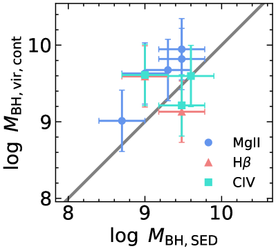
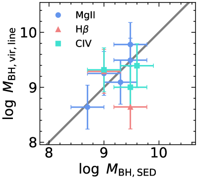
Compared the improved virial BH masses (with a 0.4 dex systematic scatter) against SED masses independently derived from modeling the accretion disk (0.3 dex systematic uncertainty; Paliya et al. 2020). A significant discrepancy would imply deviation from the standard disk (e.g., due to high BH spins) in high-redshift blazars. We do not find a statistically significant discrepancy given the sample size.
-
3.
Measured Eddington ratios and bolometric luminosities from the H and/or Mg II 2800 broad lines and line luminosities for high-redshift blazars that are robust to beaming effects (Calderone et al., 2013). We do find any compelling evidence to suggest they are super-Eddington accretors (e.g., Begelman & Volonteri 2017; Yang et al. 2020).
Future work with a larger sample size and could help confirm or falsify our main conclusions. This work highlights the challenge of obtaining deep enough NIR spectra to detect and model the broad emission lines sufficiently to estimate BH masses using ground-based observatories. Future observations with JWST would be a compelling test for blazars at even higher redshifts.
Acknowledgements
CJB and XL acknowledge support from NASA grant 80NSSC22K0030. YS acknowledges support from NSF grant AST-2009947. This research made use of pypeit,111https://pypeit.readthedocs.io/en/latest/ a Python package for semi-automated reduction of astronomical slit-based spectroscopy (Prochaska et al., 2020c, a). This research made use of Astroquery (Ginsburg et al., 2019). This research made use of Astropy, a community-developed core Python package for Astronomy (Astropy Collaboration et al., 2018, 2013). We thank Gabriele Ghisellini, Tullia Sbarrato, and Jianfeng Wu for useful discussion. We are grateful to Lea Marcotulli and the anonymous referee for comments which improved our manuscript.
Based in part on observations obtained at the international Gemini Observatory (Program ID GN-2022A-Q-138; PI: X. Liu), a program of NSF’s NOIRLab, which is managed by the Association of Universities for Research in Astronomy (AURA) under a cooperative agreement with the National Science Foundation. on behalf of the Gemini Observatory partnership: the National Science Foundation (United States), National Research Council (Canada), Agencia Nacional de Investigación y Desarrollo (Chile), Ministerio de Ciencia, Tecnología e Innovación (Argentina), Ministério da Ciência, Tecnologia, Inovações e Comunicações (Brazil), and Korea Astronomy and Space Science Institute (Republic of Korea). This work was enabled by observations made from the Gemini North telescope, located within the Maunakea Science Reserve and adjacent to the summit of Maunakea. We are grateful for the privilege of observing the Universe from a place that is unique in both its astronomical quality and its cultural significance.
Data Availability
The unreduced spectra will be available at the Gemini Observatory Archive at https://archive.gemini.edu after the proprietary period. The fully reduced, flux calibrated spectra will be made available upon reasonable request to the authors.
References
- Ackermann et al. (2017) Ackermann M., et al., 2017, ApJ, 837, L5
- Ajello et al. (2020) Ajello M., et al., 2020, ApJ, 892, 105
- Astropy Collaboration et al. (2013) Astropy Collaboration et al., 2013, A&A, 558, A33
- Astropy Collaboration et al. (2018) Astropy Collaboration et al., 2018, AJ, 156, 123
- Atwood et al. (2009) Atwood W. B., et al., 2009, ApJ, 697, 1071
- Begelman & Volonteri (2017) Begelman M. C., Volonteri M., 2017, MNRAS, 464, 1102
- Belladitta et al. (2022) Belladitta S., et al., 2022, A&A, 660, A74
- Calderone et al. (2013) Calderone G., Ghisellini G., Colpi M., Dotti M., 2013, MNRAS, 431, 210
- Celotti & Ghisellini (2008) Celotti A., Ghisellini G., 2008, MNRAS, 385, 283
- Clough et al. (2005) Clough S. A., Shephard M. W., Mlawer E. J., Delamere J. S., Iacono M. J., Cady-Pereira K., Boukabara S., Brown P. D., 2005, J. Quant. Spectrosc. Radiative Transfer, 91, 233
- Flesch (2015) Flesch E. W., 2015, Publ. Astron. Soc. Australia, 32, e010
- Ghisellini & Tavecchio (2015) Ghisellini G., Tavecchio F., 2015, MNRAS, 448, 1060
- Ghisellini et al. (2013) Ghisellini G., et al., 2013, MNRAS, 428, 1449
- Ghisellini et al. (2014) Ghisellini G., Tavecchio F., Maraschi L., Celotti A., Sbarrato T., 2014, Nature, 515, 376
- Ginsburg et al. (2019) Ginsburg A., et al., 2019, AJ, 157, 98
- Guo et al. (2018) Guo H., Shen Y., Wang S., 2018, PyQSOFit: Python code to fit the spectrum of quasars (ascl:1809.008)
- Horne (1986) Horne K., 1986, PASP, 98, 609
- Inayoshi et al. (2020) Inayoshi K., Visbal E., Haiman Z., 2020, ARA&A, 58, 27
- Johnson & Haardt (2016) Johnson J. L., Haardt F., 2016, Publ. Astron. Soc. Australia, 33, e007
- Jun et al. (2015) Jun H. D., et al., 2015, ApJ, 806, 109
- Marcotulli et al. (2020) Marcotulli L., et al., 2020, ApJ, 889, 164
- McKinney et al. (2014) McKinney J. C., Tchekhovskoy A., Sadowski A., Narayan R., 2014, MNRAS, 441, 3177
- Natarajan (2014) Natarajan P., 2014, General Relativity and Gravitation, 46, 1702
- Paliya et al. (2020) Paliya V. S., Ajello M., Cao H. M., Giroletti M., Kaur A., Madejski G., Lott B., Hartmann D., 2020, ApJ, 897, 177
- Prochaska et al. (2020a) Prochaska J. X., et al., 2020a, pypeit/PypeIt: Release 1.0.0, doi:10.5281/zenodo.3743493
- Prochaska et al. (2020b) Prochaska J. X., Hennawi J. F., Westfall K. B., Cooke R. J., Wang F., Hsyu T., Davies F. B., Farina E. P., 2020b, arXiv e-prints, p. arXiv:2005.06505
- Prochaska et al. (2020c) Prochaska J. X., et al., 2020c, Journal of Open Source Software, 5, 2308
- Reines & Comastri (2016) Reines A. E., Comastri A., 2016, Publ. Astron. Soc. Australia, 33, e054
- Richards et al. (2006) Richards G. T., et al., 2006, ApJS, 166, 470
- Runnoe et al. (2012) Runnoe J. C., Brotherton M. S., Shang Z., 2012, MNRAS, 422, 478
- Sbarrato et al. (2015) Sbarrato T., Ghisellini G., Tagliaferri G., Foschini L., Nardini M., Tavecchio F., Gehrels N., 2015, MNRAS, 446, 2483
- Sa̧dowski et al. (2014) Sa̧dowski A., Narayan R., McKinney J. C., Tchekhovskoy A., 2014, MNRAS, 439, 503
- Shakura & Sunyaev (1973) Shakura N. I., Sunyaev R. A., 1973, A&A, 24, 337
- Shaw et al. (2012) Shaw M. S., et al., 2012, ApJ, 748, 49
- Shen (2013) Shen Y., 2013, Bulletin of the Astronomical Society of India, 41, 61
- Shen & Liu (2012) Shen Y., Liu X., 2012, ApJ, 753, 125
- Shen et al. (2011) Shen Y., et al., 2011, ApJS, 194, 45
- Shen et al. (2019) Shen Y., et al., 2019, ApJS, 241, 34
- Urry & Padovani (1995) Urry C. M., Padovani P., 1995, PASP, 107, 803
- Vestergaard & Peterson (2006) Vestergaard M., Peterson B. M., 2006, ApJ, 641, 689
- Vestergaard & Wilkes (2001) Vestergaard M., Wilkes B. J., 2001, ApJS, 134, 1
- Volonteri et al. (2015) Volonteri M., Silk J., Dubus G., 2015, ApJ, 804, 148
- Wang et al. (2021) Wang F., et al., 2021, ApJ, 907, L1
- Wu et al. (2004) Wu X. B., Wang R., Kong M. Z., Liu F. K., Han J. L., 2004, A&A, 424, 793
- Yang et al. (2020) Yang X., et al., 2020, ApJ, 904, 200
- van Dokkum et al. (2012) van Dokkum P. G., Bloom J., Tewes M., 2012, L.A.Cosmic: Laplacian Cosmic Ray Identification, Astrophysics Source Code Library, record ascl:1207.005 (ascl:1207.005)
Appendix A NIR spectra


