Gelfand-Tsetlin Bases for Elliptic Quantum Groups

Hitoshi Konno and Kohei Motegi

Tokyo University of Marine Science and Technology,
Etchujima 2-1-6, Koto-Ku, Tokyo, 135-8533, Japan

E-mail: [email protected]: [email protected]

Abstract

We study the level-0 representations of the elliptic quantum group $U_{q,p}(\widehat{{\mathfrak{gl}}}_{N})$ . We give a classification theorem of the finite-dimensional irreducible representations of $U_{q,p}(\widehat{{\mathfrak{gl}}}_{N})$ in terms of the theta function analogue of the Drinfeld polynomial for the quantum affine algebra $U_{q}(\widehat{\mathfrak{gl}}_{N})$ . We also construct the Gelfand-Tsetlin bases for the level-0 $U_{q,p}(\widehat{{\mathfrak{gl}}}_{N})$ -modules following the work by Nazarov-Tarasov for the Yangian $Y({\mathfrak{gl}}_{N})$ -modules. This is a construction in terms of the Drinfeld generators. For the case of tensor product of the vector representations, we give another construction of the Gelfand-Tsetlin bases in terms of the $L$ -operators and make a connection between the two constructions. We also compare them with those obtained by the first author by using the $\mathfrak{S}_{n}$ -action realized by the elliptic dynamical $R$ -matrix on the standard bases. As a byproduct, we obtain an explicit formula for the partition functions of the corresponding 2-dimensional square lattice model in terms of the elliptic weight functions of type $A_{N-1}$ .

1 Introduction

The classification theorem of the finite-dimensional irreducible representations of the Lie algebra ${\mathfrak{gl}_{N}}={\mathfrak{gl}}(N,{\mathbb{C}})$ in terms of the dominant integral weights and the construction of the Gelfand-Tsetlin bases are the most important results in the classical representation theory. An extension of the former to the quantum groups, the Yangian $Y({\mathfrak{gl}_{N}})$ and the quantum affine algebra $U_{q}(\widehat{\mathfrak{gl}}_{N})$ , was initiated by Tarasov[33], stated by Drinfeld [8] and established by Chari and Pressley [3, 4, 5, 6]. There the classification is given in terms of the polynomials called the Drinfeld polynomials, which can be regarded as a generating functions of a set of complex numbers specifying the highest weight. To prove the theorem, for example for $U_{q}(\widehat{\mathfrak{gl}}_{N})$ , one needs careful studies of the embedding structure $U_{q}({\mathfrak{gl}_{N}})\ \hookrightarrow\ U_{q}(\widehat{\mathfrak{gl}}_{N})$ , the evaluation homomorphism $ev_{a}:U_{q}(\widehat{\mathfrak{gl}}_{N})\ \mapsto\ U_{q}({\mathfrak{gl}_{N}})$ as well as the isomorphism [8, 2] between the two realizations of $U_{q}(\widehat{\mathfrak{gl}}_{N})$ , i.e. the Drinfeld-Jimbo realization[7, 14] and the Drinfeld realization[8]. For elliptic quantum groups, only a partial result for $U_{q,p}(\widehat{\mathfrak{sl}}_{2})$ was obtained by using the evaluation homomorphism $U_{q,p}(\widehat{\mathfrak{sl}}_{2})\ \mapsto\ U_{q}(\widehat{\mathfrak{sl}}_{2})$ [21]. One of the purpose of this paper is to give a complete exposition of the necessary structures of the elliptic quantum groups $U_{q,p}(\widehat{\mathfrak{gl}}_{N})$ and $U_{q,p}(\widehat{\mathfrak{sl}}_{N})$ , and establish an elliptic version of the classification theorem.

To construct the Gelfand-Tsetlin bases for the elliptic quantum groups is the other purpose of this paper. The Gelfand-Tsetlin bases[12] of finite-dimensional irreducible representations of quantum groups were constructed for the Yangian $Y({\mathfrak{gl}}_{N})$ [28, 29, 27] and the quantum group $U_{q}({\mathfrak{gl}_{N}})$ [15, 35]. In particular, the constructions in terms of the quantum minor determinants of the $L$ -operators, or equivalently the Drinfeld generators of $Y({\mathfrak{gl}}_{N})$ , developed by Nazarov-Tarasov [29] and Molev [27] are important for us, because they can be extended to the elliptic case straightforwardly. For the elliptic quantum groups $U_{q,p}(\widehat{\mathfrak{gl}}_{N})$ and $E_{q,p}(\widehat{\mathfrak{gl}}_{N})$ , the quantum minor determinants of the $L$ -operators and their various properties were studied in [23].

On the other hand, recently, the Gelfand-Tsetlin bases of the tensor product of the vector representations have been attracting a lot of attention in geometric representation theory of quantum groups. There the Gelfand-Tsetlin bases are identified with the fixed point bases (classes) of the equivariant cohomology, $\mathrm{K}$ -theory and elliptic cohomology of quiver varieties corresponding to the quantum groups. See for example [24]. A key to this is the identification of the weight functions in the representation theory of quantum groups [13, 31, 24, 32] with the stable envelopes in the geometry of quiver varieties[26, 30, 1]. In fact, it has been shown for the case of the elliptic quantum group $U_{q,p}(\widehat{{\mathfrak{gl}}}_{N})$ that the Gelfand-Tsetlin bases are obtained by transforming the standard bases with the change of basis matrix given by the elliptic weight functions[24] (see also [31] for the affine quantum group case).

In this paper, we extend the construction of the Gelfand-Tsetlin bases to arbitrary level-0 $U_{q,p}(\widehat{{\mathfrak{gl}}}_{N})$ -modules whose weights are labelled by the Gelfand-Tsetlin patterns. We give a general construction in terms of the Drinfeld generators following the results in [29]. For the tensor product of the vector representations, we also give another construction in terms of the $L$ -operators and make a connection to the general construction. We also make a connection to the one obtained in [24], where the Gelfand-Tsetlin bases were constructed by using the action of the permutation group $\mathfrak{S}_{n}$ realized by the elliptic dynamical $R$ -matrix on the tensor product space. As a byproduct, we obtain an explicit evaluation of the partition functions of the 2-dimensional square lattice statistical model defined by the $R$ -matrix in terms of the elliptic weight functions.

This paper is organized as follows. In Section 2, we expose some properties of the elliptic quantum groups $U_{q,p}(\widehat{\mathfrak{gl}}_{N})$ , $U_{q,p}(\widehat{\mathfrak{sl}}_{N})$ and $E_{q,p}(\widehat{\mathfrak{gl}}_{N})$ . In Section 3, we give a proof of the classification theorem of level-0 finite-dimensional irreducible representations of the elliptic quantum groups. In Section 4, we present an explicit and complete example of the classification of all finite-dimensional irreducible representations of $U_{q,p}(\widehat{\mathfrak{gl}}_{2})$ and their Gelfand-Tsetlin bases. In Section 4, we give a general construction of the Gelfand-Tsetlin bases for $U_{q,p}(\widehat{\mathfrak{gl}}_{N})$ -modules in terms of the Drinfeld generators. In Section 5, we give the second construction of the Gelfand-Tsetlin bases for the case of the tensor product of the vector representations of $U_{q,p}(\widehat{\mathfrak{gl}}_{N})$ in terms of the $L$ -operators. We make a connection of them to the general construction as well as the one obtained in [24]. By considering the change of basis matrices, we obtain an explicit evaluation of the partition function of the statistical model in terms of the elliptic weight functions.

2 Elliptic Quantum Groups $U_{q,p}(\widehat{{\mathfrak{gl}}}_{N})$ and $E_{q,p}(\widehat{\mathfrak{gl}}_{N})$

In this section, we review the elliptic quantum groups $U_{q,p}(\widehat{{\mathfrak{gl}}}_{N})$ and $E_{q,p}(\widehat{\mathfrak{sl}}_{N})$ following [23]. In particular we summarize embeddings of $U_{q}({\mathfrak{gl}}_{N})$ to $U_{q}(\widehat{\mathfrak{gl}}_{N})$ and further to $U_{q,p}(\widehat{{\mathfrak{gl}}}_{N})$ as well as evaluation homomorphisms from $U_{q,p}(\widehat{{\mathfrak{gl}}}_{N})$ to $U_{q}(\widehat{\mathfrak{gl}}_{N})$ and further to $U_{q}({\mathfrak{gl}}_{N})$ . We also summarize an isomorphism between $U_{q,p}(\widehat{{\mathfrak{gl}}}_{N})$ and $E_{q,p}(\widehat{{\mathfrak{gl}}}_{N})$ and list some formulas on quantum minor determinants.

2.1 Preliminaries

Let $A=(a_{ij})$ $(0\leq i,j\leq N-1)$ be the generalized Cartan matrix of the affine Lie algebra $\widehat{\mathfrak{sl}}_{N}=\widehat{\mathfrak{sl}}(N,\mathbb{C})$ . Let $\mathfrak{h}=\widetilde{\mathfrak{h}}\oplus\mathbb{C}d$ , $\widetilde{\mathfrak{h}}=\overline{\mathfrak{h}}\oplus\mathbb{C}c$ , $\overline{\mathfrak{h}}=\oplus_{i=1}^{N-1}\mathbb{C}h_{i}$ be the Cartan subalgebras of $\widehat{\mathfrak{sl}}_{N}$ , and $\mathfrak{h}^{*}=\widetilde{\mathfrak{h}}^{*}\oplus\mathbb{C}\delta$ , $\widetilde{\mathfrak{h}}^{*}=\overline{\mathfrak{h}}^{*}\oplus\mathbb{C}\Lambda_{0}$ , $\overline{\mathfrak{h}}^{*}=\oplus_{i=1}^{N-1}\mathbb{C}\overline{\Lambda}_{i}$ their duals. Let $\mathcal{Q}=\oplus_{i=1}^{N-1}\mathbb{Z}\alpha_{i}$ be the root lattice and $\mathcal{P}=\oplus_{i=1}^{N-1}\mathbb{Z}\overline{\Lambda}_{i}$ the weight lattice. The pairings between $\delta,\Lambda_{0}$ , $\alpha_{i},\overline{\Lambda}_{i}$ $(1\leq i\leq N-1)\in\mathfrak{h}^{*}$ are given by

\displaystyle\langle\alpha_{i},h_{j}\rangle=a_{ji},\ \langle\delta,d\rangle=\langle\Lambda_{0},c\rangle=1,\ \langle\overline{\Lambda}_{i},h_{j}\rangle=\delta_{i,j},

(2.1)

and the other pairings are 0. An element $\lambda$ in ${\cal P}^{+}:=\oplus_{i=1}^{N-1}\mathbb{Z}_{\geq 0}\overline{\Lambda}_{i}$ is called a dominant integral weight. Let $\{\epsilon_{j}\ (1\leq j\leq N)\}$ be an orthonormal basis in $\mathbb{R}^{N}$ with the inner product $(\epsilon_{j},\epsilon_{k})=\delta_{j,k}$ . We set $\overline{\epsilon}_{j}=\epsilon_{j}-\sum_{k=1}^{N}\epsilon_{k}/N$ , and realize the simple roots by $\alpha_{j}=\overline{\epsilon}_{j}-\overline{\epsilon}_{j+1}$ $(1\leq j\leq N-1)$ and the fundamental weights by $\Lambda_{j}=\overline{\epsilon}_{1}+\dots+\overline{\epsilon}_{j}$ $(1\leq j\leq N-1)$ . In order to discuss $\widehat{\mathfrak{gl}}_{N}$ , we consider $\overline{\mathfrak{H}}^{*}=\oplus_{l=1}^{N}{\mathbb{C}}\epsilon_{l}$ and define $h_{\epsilon_{l}}$ $(1\leq l\leq N)$ by $h_{i}=h_{\epsilon_{i}}-h_{\epsilon_{i+1}}$ . We set $\overline{\mathfrak{H}}=\oplus_{l=1}^{N}{\mathbb{C}}h_{\epsilon_{l}}$ . We regard $\overline{\mathfrak{H}}\oplus\overline{\mathfrak{H}}^{*}$ as the Heisenberg algebra by

\displaystyle[h_{\alpha},\beta]=(\alpha,\beta),\ \ \ [h_{\alpha},h_{\beta}]=[\alpha,\beta]=0,\ \ \ \alpha,\beta\in\overline{\mathfrak{H}}^{*}.

(2.2)

Let $\{P_{\alpha},Q_{\beta}\}$ $(\alpha,\beta\in\overline{\mathfrak{H}}^{*})$ be the Heisenberg algebra defined by

\displaystyle[P_{\alpha},Q_{\beta}]=(\alpha,\beta),\ \ \ [P_{\alpha},P_{\beta}]=[Q_{\alpha},Q_{\beta}]=0.

(2.3)

We also set ${\cal R}_{Q}=\oplus_{l=1}^{N}{\mathbb{C}}Q_{\epsilon_{l}}$ and denote by ${\mathbb{C}}[{\cal R}_{Q}]$ the group ring of ${\cal R}_{Q}$ . Note that for $e^{Q_{\alpha}},e^{Q_{\beta}}\in{\mathbb{C}}[{\cal R}_{Q}]$ one has $e^{Q_{\alpha}}e^{Q_{\beta}}=e^{Q_{\alpha}+Q_{\beta}}\in{\mathbb{C}}[{\cal R}_{Q}]$ .

We define the commutative algebra $H$ as $H=\widetilde{\mathfrak{h}}\oplus\left(\oplus_{l=1}^{N}{\mathbb{C}}P_{\epsilon_{l}}\right)$ , and its dual space $H^{*}=\widetilde{\mathfrak{h}}^{*}\oplus\Big{(}\oplus_{j=1}^{N}\mathbb{C}Q_{{\epsilon}_{j}}\Big{)}$ . Then define $\mathbb{F}=\mathcal{M}_{H^{*}}$ to be the field of meromorphic functions on $H^{*}$ .

For $x\in{\mathbb{C}}$ , we set ${[x]_{q}=\frac{q^{x}-q^{-x}}{q-q^{-1}}}$ . Let $q_{1},q_{2},\cdots,q_{k}\in{\mathbb{C}}^{\times}$ satisfying $|q_{1}|,|q_{2}|,\cdots,|q_{k}|<1$ . We introduce the $q$ -infinite product

\displaystyle(x;q_{1},q_{2},\cdots,q_{k})_{\infty}=\prod_{n_{1},n_{2},\cdots,n_{k}=0}^{\infty}(1-xq_{1}^{n_{1}}q_{2}^{n_{2}}\cdots q_{k}^{n_{k}}).

(2.4)

In particular, the $k=1$ case gives

\displaystyle(x;q)_{\infty}=\prod_{n=0}^{\infty}(1-xq^{n}).

(2.5)

Let $p$ be a generic complex number satisfying $|p|<1$ , and introduce the Jacobi’s odd theta functions as

\displaystyle\Theta_{p}(z)=(z;p)_{\infty}(p/z;p)_{\infty}(p;p)_{\infty}.

(2.6)

It is also convenient to use

\displaystyle\theta(z)=-z^{-1/2}\Theta_{p}(z).

(2.7)

We also use the elliptic Gamma function defined by

\displaystyle\Gamma(z;p,q)=\frac{(pq/z;p,q)_{\infty}}{(z;p,q)_{\infty}}\qquad|p|,|q|<1.

(2.8)

This satisfies

\displaystyle\Gamma(pz;p,q)=\frac{\Theta_{q}(z)}{(q;q)_{\infty}}\Gamma(z;p,q),\qquad\Gamma(qz;p,q)=\frac{\Theta_{p}(z)}{(p;p)_{\infty}}\Gamma(z;p,q).

(2.9)

2.2 The elliptic dynamical $R$ -matrix of the $\widehat{{\mathfrak{gl}}}_{N}$ type

Let $\displaystyle\widehat{V}=\bigoplus_{j=1}^{N}{\mathbb{F}}v_{j}$ be the $N$ -dimensional vector space over ${\mathbb{F}}$ and set $\widehat{V}_{z}:=\widehat{V}[z,z^{-1}]$ . We assume $e^{Q_{\alpha}}\cdot v_{j}=v_{j}$ . We consider the elliptic dynamical $R$ -matrix ${R}^{+}(z,\Pi)\in\mathrm{End}(\widehat{V}_{z_{1}}\otimes\widehat{V}_{z_{2}})$ given by

$\displaystyle\displaystyle{R}^{+}(z,\Pi)=$	$\displaystyle\rho^{+}(z)\overline{R}(z,\Pi),$	(2.10)
$\displaystyle\displaystyle\overline{R}(z,\Pi)=$	$\displaystyle\sum_{j=1}^{N}E_{jj}\otimes E_{jj}+\sum_{1\leq j_{1}<j_{2}\leq N}\Biggl{(}b(z,\Pi_{j_{1},j_{2}})E_{j_{1},j_{1}}\otimes E_{j_{2},j_{2}}+\overline{b}(z)E_{j_{2},j_{2}}\otimes E_{j_{1},j_{1}}$
	$\displaystyle+c(z,\Pi_{j_{1},j_{2}})E_{j_{1},j_{2}}\otimes E_{j_{2},j_{1}}+\overline{c}(z,\Pi_{j_{1},j_{2}})E_{j_{2},j_{1}}\otimes E_{j_{1},j_{2}}\Biggr{)},$	(2.11)

where $E_{i,j}v_{\mu}=\delta_{j,\mu}v_{i}$ , and we set $\Pi_{j,k}=q^{2(P+h)_{j,k}}$ , $(P+h)_{j,k}:=(P+h)_{{\epsilon}_{j}}-(P+h)_{{\epsilon}_{k}}$ , and

$\displaystyle\displaystyle\rho^{+}(z)$	$\displaystyle=q^{-(N-1)/N}\frac{\Gamma(z;q^{2N},p)\Gamma(q^{2N}z;q^{2N},p)}{\Gamma(q^{2}z;q^{2N},p)\Gamma(q^{2N}q^{-2}z;q^{2N},p)},$	(2.12)
$\displaystyle b(z,\Pi)$	$\displaystyle=\frac{\theta(q^{2}\Pi)\theta(q^{-2}\Pi)\theta(z)}{\theta(\Pi)^{2}\theta(q^{2}z)},\ \ \ \overline{b}(z)=\frac{\theta(z)}{\theta(q^{2}z)},$	(2.13)
$\displaystyle c(z,\Pi)$	$\displaystyle=\frac{\theta(q^{2})\theta(z\Pi)}{\theta(\Pi)\theta(q^{2}z)},\ \ \ \overline{c}(z,\Pi)=\frac{\theta(q^{2})\theta(z\Pi^{-1})}{\theta(\Pi^{-1})\theta(q^{2}z)}.$	(2.14)

The $R$ -matrix $\overline{R}^{+}(z,q^{2s})$ satisfies the dynamical Yang-Baxter equation

	$\displaystyle\overline{R}^{+(12)}(z_{1}/z_{2},q^{2(s+h^{(3)})})\overline{R}^{+(13)}(z_{1}/z_{3},q^{2s})\overline{R}^{+(23)}(z_{2}/z_{3},q^{2(s+h^{(1)})})$
	$\displaystyle=\overline{R}^{+(23)}(z_{2}/z_{3},q^{2s})\overline{R}^{+(13)}(z_{1}/z_{3},q^{2(s+h^{(2)})})\overline{R}^{+(12)}(z_{1}/z_{2},q^{2s}),$		(2.15)

where $q^{2h_{j,k}^{(\ell)}}$ acts on the $\ell$ -th tensor space $\widehat{V}_{z_{l}}$ by $q^{2h_{j,k}^{(\ell)}}v_{\mu}=q^{2\langle\overline{\epsilon}_{\mu},h_{j,k}\rangle}v_{\mu}$ .

2.3 The elliptic algebra $U_{q,p}(\widehat{{\mathfrak{gl}}}_{N})$

Definition 2.1.

The elliptic algebra $U_{q,p}(\widehat{\mathfrak{gl}}_{N})$ is a topological algebra over ${\mathbb{F}}[[p]]$ generated by $e_{j,m},f_{j,m},k_{l,m}$ , $(1\leq j\leq N-1,1\leq l\leq N,m\in{\mathbb{Z}})$ and the central elements $q^{\pm c/2}$ . The defining relations are given in terms of the following generating functions called the elliptic currents.

	$\displaystyle e_{j}(z)=\sum_{m\in{\mathbb{Z}}}e_{j,m}z^{-m},\quad f_{j}(z)=\sum_{m\in{\mathbb{Z}}}f_{j,m}z^{-m},$		(2.16)
	$\displaystyle k_{l}^{+}(z)=\sum_{m\in{\mathbb{Z}}_{\geq 0}}k_{l,-m}z^{m}+\sum_{m\in{\mathbb{Z}}_{>0}}k_{l,m}p^{m}z^{-m},$		(2.17)
	$\displaystyle k^{-}_{l}(z)=q^{2h_{\epsilon_{l}}}k^{+}_{l}(zpq^{-c}).$		(2.18)

The relations are given in Appendix A.1¹¹1Through this paper we do not consider the derivation operator ${\widehat{d}}$ ..

In the following, we set $p^{*}=pq^{-2c}$ . Let ${\cal E}^{l}_{m}\ (1\leq l\leq N,m\in{\mathbb{Z}}_{\not=0})$ be operators satisfying²²2 Our ${\cal E}^{l}_{m}$ is $(q^{m}-q^{-m})^{2}{\cal E}^{+l}_{m}$ in [10, 23].

	$\displaystyle[{\cal E}^{l}_{m},{\cal E}^{l}_{n}]=\delta_{m+n,0}\frac{[cm]_{q}[(N-1)m]_{q}(q^{m}-q^{-m})^{2}}{m[m]_{q}[Nm]_{q}}\frac{1-p^{m}}{1-p^{*m}}q^{-cm},$		(2.19)
	$\displaystyle[{\cal E}^{k}_{m},{\cal E}^{l}_{n}]=-\delta_{m+n,0}q^{-{\rm sgn}(k-l)Nm+(k-l)m}\frac{[cm]_{q}(q^{m}-q^{-m})^{2}}{m[Nm]_{q}}\frac{1-p^{m}}{1-p^{*m}}q^{-cm},$		(2.20)
	$\displaystyle\sum_{l=1}^{N}q^{(l-1)m}{\cal E}^{l}_{m}=0.$		(2.21)

Then one can realize $k^{+}_{l}(z)$ as

\displaystyle k^{+}_{l}(z)

\displaystyle=

\displaystyle K^{+}_{\epsilon_{l}}\exp\left\{-\sum_{m>0}\frac{{\cal E}^{l}_{-m}}{1-p^{m}}(q^{l}z)^{m}\right\}\exp\left\{\sum_{m>0}\frac{p^{m}{\cal E}^{l}_{m}}{1-p^{m}}(q^{l}z)^{-m}\right\}.

(2.22)

Here, expanding $k_{l,m}\in U_{q,p}(\widehat{\mathfrak{gl}}_{N})$ in $p$

\displaystyle k_{l,m}=\sum_{r\in{\mathbb{Z}}_{\geq 0}}k^{(r)}_{l,m}p^{r},\qquad 1\leq l\leq N,\ m\in{\mathbb{Z}},

(2.23)

we have

\displaystyle K^{+}_{\epsilon_{l}}=k^{(0)}_{l,0}.

(2.24)

Let us set

\displaystyle K(z)=k^{+}_{1}(z)k^{+}_{2}(q^{-2}z)\cdots k^{+}_{N}(q^{-2(N-1)}z).

Then $K(z)$ belongs to the center of $U_{q,p}(\widehat{\mathfrak{gl}}_{N})$ (Proposition 3.2 in [23]). This can also be verified from (2.21), (2.22) and the fact that $\prod_{l=1}^{N}q^{-h_{\epsilon_{l}}}$ belongs to the center.

Let $U^{D}_{q}(\widehat{\mathfrak{gl}}_{N})$ be the quantum affine algebra over ${\mathbb{C}}$ generated by the Drinfeld generators $X^{\pm}_{j,m},K^{\pm}_{l,m},q^{\pm c/2}$ . The defining relations can be seen in Appendix A in [23]. We set

\displaystyle X^{\pm}_{j}(z)=\sum_{m\in{\mathbb{Z}}}X^{\pm}_{j,m}z^{-m},\qquad K^{\pm}_{l}(z)=\sum_{m\in{\mathbb{Z}}_{\geq 0}}K^{\pm}_{l,\mp m}z^{\pm m}.

Note the relation $K^{+}_{l,0}K^{-}_{l,0}=1=K^{-}_{l,0}K^{+}_{l,0}$ .

Let us introduce the currents $u^{+}_{\epsilon_{l}}(z,p)\in U_{q,p}(\widehat{\mathfrak{gl}}_{N})[[p]][[z]]$ , $u^{-}_{\epsilon_{l}}(z,p)\in U_{q,p}(\widehat{\mathfrak{gl}}_{N})[[p]][[z^{-1}]]$ $(1\leq l\leq N)$ by

	$\displaystyle u^{+}_{\epsilon_{l}}(z,p)=\exp\left\{\sum_{m>0}\frac{(pq^{-c})^{m}{\cal E}^{l}_{-m}}{1-p^{m}}\;z^{m}\right\},$		(2.25)
	$\displaystyle u^{-}_{\epsilon_{l}}(z,p)=\exp\left\{-\sum_{m>0}\frac{p^{m}{\cal E}^{l}_{m}}{1-p^{m}}\;z^{-m}\right\},$		(2.26)

and set

\displaystyle u_{j}^{\pm}(z,p)=u^{\pm}_{\epsilon_{j}}(z,p)u^{\pm}_{\epsilon_{j+1}}(qz,p)^{-1}\qquad(1\leq j\leq N-1).

(2.27)

These are well defined elements in $(U_{q,p}(\widehat{\mathfrak{gl}}_{N})[[p]])[[z,z^{-1}]]$ in the $p$ -adic topology.

Theorem 2.2.

The map $\pi_{p}:({\mathbb{F}}\otimes_{\mathbb{C}}U^{D}_{q}(\widehat{\mathfrak{gl}}_{N}))\sharp{\mathbb{C}}[{\cal R}_{Q}]\to U_{q,p}(\widehat{\mathfrak{gl}}_{N})$ defined by

	$\displaystyle\pi_{p}(X^{+}_{j}(z)e^{-Q_{j}})=u_{j}^{+}(z,p)e_{j}^{+}(z),$
	$\displaystyle\pi_{p}(X^{-}_{j}(z))=f_{j}^{-}(z)u_{j}^{-}(z,p),$
	$\displaystyle\pi_{p}(K^{+}_{l}(z)e^{-Q_{\epsilon_{l}}})=u_{\epsilon_{l}}^{+}(q^{-c+l}z,p)k^{+}_{l}(z)u_{\epsilon_{l}}^{-}(q^{l}z,p),$
	$\displaystyle\pi_{p}(K^{-}_{l}(z)e^{-Q_{\epsilon_{l}}})=u_{\epsilon_{l}}^{+}(q^{l}z,p)k^{-}_{l}(z)u_{\epsilon_{l}}^{-}(q^{-c+l}z,p).$

is an algebra homomorphism. Here the smash product $\sharp$ is defined as follows.

	$\displaystyle g(P,P+h)a\otimes e^{Q_{\alpha}}\cdot f(P,P+h)b\otimes e^{Q_{\beta}}$
	$\displaystyle\quad=g(P,P+h)f(P-\langle Q_{\alpha},P\rangle,P+h-\langle Q_{\alpha}+{\rm wt}(a),P+h\rangle)ab\otimes e^{Q_{\alpha}+Q_{\beta}}$

where ${\rm wt}({a})\in\bar{\mathfrak{h}}^{*}$ s.t. $q^{h}aq^{-h}=q^{\langle{\rm wt}({a}),h\rangle}a$ for $a,b\in U_{q}(\widehat{\mathfrak{g}}),f(P),g(P)\in{\mathbb{F}},e^{Q_{\alpha}},e^{Q_{\beta}}\in{\mathbb{C}}[{\cal R}_{Q}]$ .

In particular, one obtains the following identifications.

Corollary 2.3.

	$\displaystyle K^{+}_{l,0}e^{-Q_{\epsilon_{l}}}=q^{-2h_{\epsilon_{l}}}K^{-}_{l,0}e^{-Q_{\epsilon_{l}}}=K^{+}_{\epsilon_{l}}=q^{-h_{\epsilon_{l}}}e^{-Q_{\epsilon_{l}}},$		(2.28)
	$\displaystyle\pi_{p}(K^{+}_{l}(z))=q^{-h_{\epsilon_{l}}}\exp\left\{-\sum_{m>0}\frac{1-p^{*m}}{1-p^{m}}{\cal E}^{l}_{-m}(q^{l}z)^{m}\right\}\ \in U_{q,p}(\widehat{\mathfrak{gl}}_{N})[[z]],$		(2.29)
	$\displaystyle\pi_{p}(K^{-}_{l}(z))=q^{h_{\epsilon_{l}}}\exp\left\{\sum_{m>0}{\cal E}^{l}_{m}(q^{l-c}z)^{-m}\right\}\ \in U_{q,p}(\widehat{\mathfrak{gl}}_{N})[[z^{-1}]].$		(2.30)

One also has the inverse of $\pi_{p}$ ( Sec.5.2 in [23]). Hence one obtains the isomorphism
${U_{q,p}(\widehat{\mathfrak{gl}}_{N})\cong({\mathbb{F}}\otimes_{{\mathbb{C}}}U^{D}_{q}(\widehat{\mathfrak{gl}}_{N}))\sharp{\mathbb{C}}[{\cal R}_{Q}]}$ . In the below we set $K_{\epsilon_{l}}=K^{+}_{l,0}=(K^{-}_{l,0})^{-1}=q^{-h_{\epsilon_{l}}}$ .

The quantum affine algebra associated with $\widehat{\mathfrak{gl}}_{N}$ has the other realization $U^{DJ}(\widehat{\mathfrak{gl}}_{N})$ called the Drinfeld-Jimbo realization[7, 14]. This is generated by the Chevalley type generators ${\cal X}^{\pm}_{r},{\cal K}_{\epsilon_{l}},q^{\pm c/2}\ (0\leq r\leq N-1,\ 1\leq l\leq N)$ subject to

	$\displaystyle{\cal K}_{\epsilon_{l}}{\cal K}_{\epsilon_{m}}={\cal K}_{\epsilon_{m}}{\cal K}_{\epsilon_{l}},\qquad{\cal K}_{\epsilon_{l}}{\cal K}_{\epsilon_{l}}^{-1}={\cal K}_{\epsilon_{l}}^{-1}{\cal K}_{\epsilon_{l}}=1\qquad(1\leq l,m\leq N),$
	$\displaystyle{\cal K}_{\epsilon_{l}}{\cal X}^{\pm}_{r}{\cal K}_{\epsilon_{l}}^{-1}=q^{\mp\langle\alpha_{r},h_{\epsilon_{l}}\rangle}{\cal X}^{\pm}_{r},$
	$\displaystyle[{\cal X}^{+}_{r},{\cal X}^{-}_{s}]=\frac{\delta_{r,s}}{q-q^{-1}}({\cal K}_{\epsilon_{r}}^{-1}{\cal K}_{\epsilon_{r+1}}-{\cal K}_{\epsilon_{r}}{\cal K}_{\epsilon_{r+1}}^{-1}),$

where we set $\alpha_{0}=\delta-\theta$ and ${\cal K}_{\epsilon_{0}}\equiv q^{c}{\cal K}_{\epsilon_{N}}$ .

The isomorphism between $U^{D}_{q}(\widehat{\mathfrak{gl}}_{N})$ and $U^{DJ}_{q}(\widehat{\mathfrak{gl}}_{N})$ is given as follows[8, 25, 2]. Let us set in $U_{q}^{D}(\widehat{\mathfrak{gl}}_{N})$

	$\displaystyle K_{j}:=K_{\epsilon_{j}}K_{\epsilon_{j+1}}^{-1},\qquad(1\leq j\leq N-1)$		(2.31)
	$\displaystyle K_{\theta}:=K_{1}K_{2}\cdots K_{N-1}=K_{\epsilon_{1}}K_{\epsilon_{N}}^{-1}.$		(2.32)

Then one has an isomorphism of ${\mathbb{C}}$ -algebras $f:U^{DJ}_{q}(\widehat{\mathfrak{gl}}_{N})\to U^{D}_{q}(\widehat{\mathfrak{gl}}_{N})$ given by

	$\displaystyle f({\cal K}_{0})=q^{c}K_{\theta},\qquad f({\cal K}_{\epsilon_{l}})=K_{\epsilon_{l}},\qquad f({\cal X}^{\pm}_{j})=X^{\pm}_{j,0},$		(2.33)
	$\displaystyle f({\cal X}^{+}_{0})=[X^{-}_{N-1,0},[X^{-}_{N-2,0},\cdots[X^{-}_{2,0},X^{-}_{1,1}]_{q^{-1}}\cdots]_{q^{-1}}]_{q^{-1}}K_{\theta}^{-1},$		(2.34)
	$\displaystyle f({\cal X}^{-}_{0})=K_{\theta}[[\cdots[X^{+}_{1,-1},X^{+}_{2,0}]_{q}\cdots,X^{+}_{N-2,0}]_{q},X^{+}_{N-1,0}]_{q},$		(2.35)

where $[A,B]_{q^{\pm 1}}=AB-q^{\pm 1}BA$ . One also has the opposite algebra homomorphism $F:U^{D}_{q}(\widehat{\mathfrak{gl}}_{N})\to U^{DJ}_{q}(\widehat{\mathfrak{gl}}_{N})$ in the same way as in [2] for $U_{q}(\widehat{\mathfrak{sl}}_{N})$ .

It is also obvious that $U^{DJ}_{q}(\widehat{\mathfrak{gl}}_{N})$ has a subalgebra $U_{q}({\mathfrak{gl}}_{N})$ generated by ${\cal X}^{\pm}_{j},{\cal K}_{\epsilon_{l}}\ (1\leq j\leq N-1,\ 1\leq l\leq N)$ subject to

	$\displaystyle{\cal K}_{\epsilon_{l}}{\cal X}^{\pm}_{j}{\cal K}_{\epsilon_{l}}^{-1}=q^{\mp\langle\alpha_{j},h_{\epsilon_{l}}\rangle}{\cal X}^{\pm}_{j},$
	$\displaystyle[{\cal X}^{+}_{i},{\cal X}^{-}_{j}]=\frac{\delta_{i,j}}{q-q^{-1}}({\cal K}_{\epsilon_{j}}^{-1}{\cal K}_{\epsilon_{j+1}}-{\cal K}_{\epsilon_{j}}{\cal K}_{\epsilon_{j+1}}^{-1}).$

The opposite algebra homomorphism ${\rm ev}_{a}:U^{DJ}_{q}(\widehat{\mathfrak{gl}}_{N})\ \ {\longrightarrow}\ U_{q}({\mathfrak{gl}}_{N})$ was obtained by Jimbo [16]. Let us define $\widehat{E}_{ij}\in U_{q}({\mathfrak{gl}_{N}})\ (1\leq i\not=j\leq N)$ inductively by $\widehat{E}_{jj+1}={\cal X}^{+}_{j}$ , $\widehat{E}_{j+1j}={\cal X}^{-}_{j}$ and

\displaystyle\widehat{E}_{ij}=\widehat{E}_{ik}\widehat{E}_{kj}-q^{\pm 1}\widehat{E}_{kj}\widehat{E}_{ik}\qquad(i\gtrless k\gtrless j).

Then the following map gives an algebra homomorphism ${\rm ev}_{a}:U^{DJ}_{q}(\widehat{\mathfrak{gl}}_{N})\ \ {\longrightarrow}\ U_{q}({\mathfrak{gl}}_{N})[a,a^{-1}]$ with $a\in{\mathbb{C}}^{\times}$ .

	$\displaystyle{\rm ev}_{a}({\cal K}_{0})={\cal K}_{\epsilon_{1}}{\cal K}_{\epsilon_{N}}^{-1},\qquad$		(2.36)
	$\displaystyle{\rm ev}_{a}({\cal X}^{+}_{0})=aq^{-1}{\cal K}_{\epsilon_{1}}{\cal K}_{\epsilon_{N}}\widehat{E}_{N1},$		(2.37)
	$\displaystyle{\rm ev}_{a}({\cal X}^{+}_{0})=a^{-1}q{\cal K}_{\epsilon_{1}}^{-1}{\cal K}_{\epsilon_{N}}^{-1}\widehat{E}_{1N},$		(2.38)
	$\displaystyle{\rm ev}_{a}({\cal K}_{\epsilon_{l}})={\cal K}_{\epsilon_{l}},\qquad{\rm ev}_{a}({\cal X}^{\pm}_{j})={\cal X}^{\pm}_{j}\qquad(1\leq l\leq N,1\leq j\leq N-1).$		(2.39)

In summary we have the following embeddings

\displaystyle U_{q}({\mathfrak{gl}}_{N})\ \hookrightarrow\ U^{DJ}_{q}(\widehat{\mathfrak{gl}}_{N})\ \hookrightarrow\ ({\mathbb{F}}\otimes_{\mathbb{C}}U^{D}_{q}(\widehat{\mathfrak{gl}}_{N}))\sharp{\mathbb{C}}[{\cal R}_{Q}]\ \stackrel{{\scriptstyle\pi_{p}}}{{\hookrightarrow}}\ U_{q,p}(\widehat{\mathfrak{gl}}_{N}),

(2.40)

where in the middle we used $U^{DJ}_{q}(\widehat{\mathfrak{gl}}_{N})\stackrel{{\scriptstyle\cong}}{{\longrightarrow}}U^{D}_{q}(\widehat{\mathfrak{gl}}_{N})$ by Beck [2]. In particular, we have the identification

\displaystyle{\cal K}_{\epsilon_{l}}\ \mapsto\ K_{\epsilon_{l}},\quad K_{\epsilon_{l}}e^{-Q_{\epsilon_{l}}}\mapsto\ K^{+}_{\epsilon_{l}}.

(2.41)

On the other hand, we have the algebra homomorphisms of the opposite direction.

\displaystyle U_{q,p}(\widehat{\mathfrak{gl}}_{N})\ \stackrel{{\scriptstyle\pi_{p}^{-1}}}{{\longrightarrow}}\ ({\mathbb{F}}\otimes_{\mathbb{C}}U^{D}_{q}(\widehat{\mathfrak{gl}}_{N}))\sharp{\mathbb{C}}[{\cal R}_{Q}]\ \stackrel{{\scriptstyle{\rm ev}_{a}}}{{\longrightarrow}}\ ({\mathbb{F}}\otimes_{\mathbb{C}}U_{q}({\mathfrak{gl}}_{N})[a,a^{-1}])\sharp{\mathbb{C}}[{\cal R}_{Q}].

(2.42)

2.4 The elliptic algebra $U_{q,p}(\widehat{\mathfrak{sl}}_{N})$

The elliptic algebra $U_{q,p}(\widehat{\mathfrak{sl}}_{N})$ is defined as the quotient algebra

\displaystyle U_{q,p}(\widehat{\mathfrak{gl}}_{N})/<K(z)-1>.

(2.43)

Set

	$\displaystyle K^{+}_{j}:=K^{+}_{\epsilon_{j}}K^{+-1}_{\epsilon_{j+1}},$		(2.44)
	$\displaystyle\alpha_{j,m}:=\frac{1}{q-q^{-1}}\left({\cal E}^{j}_{m}-q^{-m}{\cal E}^{j+1}_{m}\right)\qquad 1\leq j\leq N-1,\ m\in{\mathbb{Z}}.$		(2.45)

One has

\displaystyle[\alpha_{i,m},\alpha_{j,n}]=\delta_{m+n,0}\frac{[a_{ij}m]_{q}[cm]_{q}}{m}\frac{1-p^{m}}{1-p^{*m}}q^{-cm}.

(2.46)

Solving (2.45) and (2.21), one obtains

	$\displaystyle{\cal E}^{j}_{m}=(q-q^{-1})\frac{q^{jm}}{[Nm]_{q}}\left(-q^{-Nm}\sum_{k=1}^{j-1}[km]_{q}\alpha_{k,m}+\sum_{k=j}^{N-1}[(N-k)m]_{q}\alpha_{k,m}\right)\quad(1\leq j\leq N-1),$
	$\displaystyle{\cal E}^{N}_{m}=-\frac{(q-q^{-1})}{[Nm]_{q}}\sum_{k=1}^{N-1}[km]_{q}\alpha_{k,m}.$		(2.47)

Let us define $\psi^{\pm}_{j}(z)\ (1\leq j\leq N-1)$ by³³3Our $\psi^{\pm}_{j}(z)$ are $\psi^{\mp}_{j}(z)$ in [18, 20].

	$\displaystyle\psi^{+}_{j}(q^{-c/2}q^{j}z):=\kappa k^{+}_{j}(z)k^{+}_{j+1}(z)^{-1},$		(2.48)
	$\displaystyle\psi^{-}_{j}(q^{-c/2}q^{j}z):=\kappa k^{-}_{j}(z)k^{-}_{j+1}(z)^{-1}$		(2.49)

with $\kappa$ given in (A.21). Then one has

	$\displaystyle{\psi}_{j}^{+}(q^{-\frac{c}{2}}z)=K^{+}_{j}\exp\left(-(q-q^{-1})\sum_{n>0}\frac{\alpha_{j,-n}}{1-p^{n}}z^{n}\right)\exp\left((q-q^{-1})\sum_{n>0}\frac{p^{n}\alpha_{j,n}}{1-p^{n}}z^{-n}\right),$
	$\displaystyle\psi^{-}_{j}(z)=q^{2h_{j}}\psi^{+}_{j}(zpq^{-c}).$		(2.50)

Definition 2.4.

The elliptic algebra $U_{q,p}(\widehat{\mathfrak{sl}}_{N})$ is a topological algebra over ${\mathbb{F}}[[p]]$ generated by $\alpha_{j,n},e_{j,m},f_{j,m}\ (1\leq j\leq N-1,n\in{\mathbb{Z}}\backslash\{0\},m\in{\mathbb{Z}})$ and the central elements $q^{\pm c/2}$ satisfying the relations in Appendix A.2.

The quantum affine algebra $U_{q}(\widehat{\mathfrak{sl}}_{N})$ is an associative algebra generated by $X^{\pm}_{j,m}\ (1\leq j\leq N-1,m\in{\mathbb{Z}})$ and $a_{j,n}$ $(n\in{\mathbb{Z}}\backslash\{0\})$ defined by

\displaystyle a_{j,n}=\left\{\begin{matrix}\alpha_{j,n}&n>0\cr\frac{1-p^{*n}}{1-p^{n}}q^{2cn}\alpha_{j,n}&n<0\cr\end{matrix}\right..

(2.51)

One finds

\displaystyle[a_{i,m},a_{j,n}]=\frac{[a_{ij}m]_{q}[cm]_{q}}{m}q^{-c|m|}\delta_{m+n,0}.

Furthermore define

\displaystyle\Phi^{\pm}_{j}(q^{j}z):=K^{\pm}_{j}(z)K^{\pm}_{j+1}(z)^{-1}.

(2.52)

Then one gets the generating functions of $a_{j,m}$ as

\displaystyle\Phi^{\pm}_{j}(z)=q^{\mp h_{j}}\exp\left\{\mp(q-q^{-1})\sum_{m>0}a_{j,\mp m}z^{\pm m}\right\}.

(2.53)

2.5 The elliptic algebra $E_{q,p}(\widehat{{\mathfrak{gl}}}_{N})$

The elliptic algebra $E_{q,p}(\widehat{{\mathfrak{gl}}}_{N})$ is generated by the $L$ -operators. Let $\bar{L}_{ij,n}\ (n\in{\mathbb{Z}},1\leq i,j\leq N)$ be abstract symbols. We define the $L$ -operator $L^{+}(z)=\sum_{1\leq i,j\leq N}E_{ij}\otimes L^{+}_{ij}(z)$ by

\displaystyle L^{+}_{ij}(z)=\sum_{n\in{\mathbb{Z}}}L_{ij,n}z^{-n},\qquad L_{ij,n}=p^{{\rm max}(n,0)}\bar{L}_{ij,n}.

(2.54)

Definition 2.5.

Let $R^{+}(z,\Pi)$ be the same $R$ matrix as in Sec.2.2. The elliptic algebra ${\cal E}=E_{q,p}(\widehat{\mathfrak{gl}}_{N})$ is a topological algebra over ${\mathbb{F}}[[p]]$ generated by $\bar{L}_{ij,n}$ and the central element $q^{\pm c/2}$ satisfying the following relations.

	$\displaystyle R^{+(12)}(z_{1}/z_{2},\Pi)L^{+(1)}(z_{1})L^{+(2)}(z_{2})=L^{+(2)}(z_{2})L^{+(1)}(z_{1})R^{+(12)}(z_{1}/z_{2},\Pi^{}),$		(2.55)
	$\displaystyle g({P+h})\bar{L}_{ij,n}=\bar{L}_{ij,n}\;g(P+h-\langle Q_{\bar{\epsilon}_{i}},P+h\rangle),$		(2.56)
	$\displaystyle g({P})\bar{L}_{ij,n}=\bar{L}_{ij,n}\;g(P-\langle Q_{\bar{\epsilon}_{j}},P\rangle),$		(2.57)

where $g({P+h}),g(P)\in{\mathbb{F}}$ and

\displaystyle L^{+(1)}(z)=L^{+}(z)\otimes{\rm id},\qquad L^{+(2)}(z)={\rm id}\otimes L^{+}(z).

The $R$ -matrix $R^{+*}(z,\Pi^{*})$ is the same as $R^{+}(z,\Pi)$ except for the replacements : theta functions $\theta(z)$ by $\theta^{*}(z):=-z^{-1/2}(z;p^{*})_{\infty}(p^{*}/z;p^{*})_{\infty}(p^{*};p^{*})_{\infty}$ and the dynamical parameters $\Pi_{k,l}$ by $\Pi^{*}_{k,l}=q^{2(P_{\epsilon_{k}}-P_{\epsilon_{l}})}$ .

We regard $L^{+}(z)\in\operatorname{End}_{\mathbb{F}}\widehat{V}_{z}\otimes{\cal E}$ . We treat (2.55) as a formal Laurent series in $z_{1}$ and $z_{2}$ . The coefficients of $z_{1},z_{2}$ are well defined in the $p$ -adic topology.

It is also convenient to introduce the dynamical $L$ -operator $L^{+}(z,\Pi^{*})$ defined by[18, 20]

\displaystyle L^{+}(z,\Pi^{*})=L^{+}(z)e^{\sum_{i=1}^{N}\pi_{V}(h_{\varepsilon_{i}})\otimes Q_{\epsilon_{i}}},

(2.58)

where $\pi_{V}(h_{\epsilon_{i}})=E_{i,i}$ . We then have the fully dynamical $RLL$ -relation[11]

	$\displaystyle R^{+(12)}(z_{1}/z_{2},{\Pi}^{}q^{2h^{(3)}})L^{+(1)}(z_{1},\Pi^{})L^{+(2)}(z_{2},{\Pi^{*}q^{2\pi_{V}(h)^{(1)}}})$
	$\displaystyle\qquad\qquad=L^{+(2)}(z_{2},\Pi^{})L^{+(1)}(z_{1},{\Pi^{}q^{2\pi_{V}(h)^{(2)}}})R^{+(12)}(z_{1}/z_{2},\Pi^{}).$		(2.59)

2.6 Isomorphism between $U_{q,p}(\widehat{\mathfrak{gl}}_{N})$ and $E_{q,p}(\widehat{\mathfrak{gl}}_{N})$

The two elliptic algebras $U_{q,p}(\widehat{\mathfrak{gl}}_{N})$ and $E_{q,p}(\widehat{\mathfrak{gl}}_{N})$ are isomorphic[23]. We briefly summarize their isomorphism.

Let us introduce $L^{-}(z)=\sum_{1\leq i,j\leq N}E_{ij}\otimes L^{-}_{ij}(z)$ by[17, 23]

	$\displaystyle L^{-}(z)=\left({\rm Ad}(q^{-2{\theta}_{V}(P)})\otimes{\rm id}\right)\left(q^{2{T}_{V}}L^{+}(zp^{*}q^{c})\right),$		(2.60)
	$\displaystyle{\theta}_{V}(P)=-\sum_{j=1}^{N-1}\left(\frac{1}{2}\pi_{V}(h_{j})\pi_{V}(h^{j})+P_{j}\pi_{V}(h^{j})\right),$		(2.61)
	$\displaystyle{T}_{V}=\sum_{j=1}^{N-1}\pi_{V}(h_{j})\otimes h^{j}.$		(2.62)

Here $({\rm Ad}X)Y=XYX^{-1}$ , $h^{j}=h_{\bar{\Lambda}_{j}}\ (j\in I)$ , $\pi_{V}(h_{j})=E_{jj}-E_{j+1j+1}$ and $\pi_{V}(h^{j})=\sum_{i=1}^{j}\pi_{V}(h_{\bar{\epsilon}_{i}})\ (j\in I)$ . Hence $L^{+}$ and $L^{-}$ are not independent operators in the elliptic algebra in contrast to the quantum affine algebra $U_{q}(\widehat{\mathfrak{gl}}_{N})$ .

One can verify the following.

Proposition 2.6.

The $L$ operators $L^{+}(z)$ and $L^{-}(z)$ satisfy the following relations.

	$\displaystyle R^{-(12)}(z_{1}/z_{2},\Pi)L^{-(1)}(z_{1})L^{-(2)}(z_{2})=L^{-(2)}(z_{2})L^{-(1)}(z_{1})R^{-(12)}(z_{1}/z_{2},\Pi^{}),$
	$\displaystyle R^{\pm(12)}(q^{\pm{c}}z_{1}/z_{2},\Pi)L^{\pm(1)}(z_{1})L^{\mp(2)}(z_{2})=L^{\mp(2)}(z_{2})L^{\pm(1)}(z_{1})R^{\pm(12)}(q^{\mp{c}}z_{1}/z_{2},\Pi^{}).$

Definition 2.7.

We define the Gauss components $E^{\pm}_{l,j}(z),F^{\pm}_{j,l}(z),K^{\pm}_{m}(z)\ (1\leq j<l\leq N,1\leq m\leq N)$ of the $L$ -operator ${L}^{\pm}(z)$ of ${\cal E}$ as follows.

	$\displaystyle{L}^{\pm}(z)=\left(\begin{array}[]{ccccc}1&F_{1,2}^{\pm}(z)&F_{1,3}^{\pm}(z)&\cdots&F_{1,N}^{\pm}(z)\\ 0&1&F_{2,3}^{\pm}(z)&\cdots&F_{2,N}^{\pm}(z)\\ \vdots&\ddots&\ddots&\ddots&\vdots\\ \vdots&&\ddots&1&F_{N-1,N}^{\pm}(z)\\ 0&\cdots&\cdots&0&1\end{array}\right)\left(\begin{array}[]{cccc}K^{\pm}_{1}(z)&0&\cdots&0\\ 0&K^{\pm}_{2}(z)&&\vdots\\ \vdots&&\ddots&0\\ 0&\cdots&0&K^{\pm}_{N}(z)\end{array}\right)$		(2.72)
	$\displaystyle\qquad\qquad\qquad\qquad\qquad\qquad\qquad\times\left(\begin{array}[]{ccccc}1&0&\cdots&\cdots&0\\ E^{\pm}_{2,1}(z)&1&\ddots&&\vdots\\ E^{\pm}_{3,1}(z)&E^{\pm}_{3,2}(z)&\ddots&\ddots&\vdots\\ \vdots&\vdots&\ddots&1&0\\ E^{\pm}_{N,1}(z)&E^{\pm}_{N,2}(z)&\cdots&E^{\pm}_{N,N-1}(z)&1\end{array}\right).$		(2.78)

In particular we call $E^{\pm}_{j+1,j}(z),F^{\pm}_{j,j+1}(z),K^{\pm}_{m}(z)$ the basic half currents.

In [23], it was shown that there are a sequence of subalgebras

\displaystyle E_{q,p}(\widehat{{\mathfrak{gl}}}_{1})\subset E_{q,p}(\widehat{{\mathfrak{gl}}}_{2})\subset\cdots\subset E_{q,p}(\widehat{{\mathfrak{gl}}}_{N}),

(2.79)

where $E_{q,p}(\widehat{{\mathfrak{gl}}}_{m})$ is generated by the coefficients of the basic half currents $E^{+}_{a+1,a}(u),F^{+}_{a,a+1}(u),K_{b}^{+}(u)$ $(N-m+1\leq a\leq N-1,\ N-m+1\leq b\leq N)$ .

In addition, the following lemma indicates that the whole Gauss components of $L^{\pm}(z)$ can be determined recursively by the basic half currents.

Lemma 2.8 ([23], Lemma 6.10).

Let $I_{a,b}=\{\ (j,k)\ |\ a\leq j\leq b-1,\ j+1\leq k\leq b\}\setminus\{(a,b)\}$ . For $2\leq l+1<m\leq N$ , $E^{+}_{m,l}(z)$ (resp. $F^{+}_{l,m}(z)$ ) is determined by $\{E^{+}_{k,j}(z)\ (j,k)\in I_{l,m},K^{+}_{j}(z)\ l\leq j\leq m\}$ (resp. $\{F^{+}_{j,k}(z)\ (j,k)\in I_{l,m},K^{+}_{j}(z)\ l\leq j\leq m\}$ ).

Now let us define the basic half currents $e_{j+1,j}^{+}(z),f_{j,j+1}^{+}(z)$ $(1\leq j\leq N-1)$ of ${\cal U}$ as follows.

Definition 2.9.

	$\displaystyle e_{j+1,j}^{+}(z)=a^{}\oint_{C^{}}\frac{dz^{\prime}}{2\pi iz^{\prime}}e_{j}(z^{\prime})\frac{{\Theta}_{p^{}}(zq^{j-c}q^{2(1-P_{\alpha_{j}})}/z^{\prime}){\Theta}_{p^{}}(q^{2})}{{\Theta}_{p^{}}(zq^{j-c}/z^{\prime}){\Theta}_{p^{}}(q^{2(P_{\alpha_{j}}-1)})},$		(2.80)
	$\displaystyle f_{j,j+1}^{+}(z)=a\oint_{C}\frac{dz^{\prime}}{2\pi iz^{\prime}}f_{j}(z^{\prime})\frac{{\Theta_{p}}(zq^{j}q^{2((P+h)_{\alpha_{j}}-1)}/z^{\prime}){\Theta_{p}}(q^{2})}{{\Theta_{p}}(zq^{j}/z^{\prime}){\Theta_{p}}(q^{2((P+h)_{\alpha_{j}}-1)})},$		(2.81)

where $C^{*}:|q^{j-c}z|<|z^{\prime}|<|p^{*-1}q^{j-c}z|$ , $C:|q^{j}z|<|z^{\prime}|<|p^{-1}q^{j}z|$ , and

\displaystyle a^{*}=q^{-1}\frac{(p^{*};p^{*})_{\infty}}{(p^{*}q^{2};p^{*})_{\infty}},\qquad a=q^{-1}\frac{(p;p)_{\infty}}{(pq^{-2};p)_{\infty}}.

(2.82)

Theorem 2.10.

The following map gives an isomorphism ${\cal U}\cong{\cal E}$ as a topological $H$ -algebra over ${\mathbb{F}}[[p]]$ .

\displaystyle e^{+}_{j+1,j}(z)\mapsto E^{+}_{j+1,j}(z),\quad f^{+}_{j,j+1}(z)\mapsto F^{+}_{j,j+1}(z),\quad k^{+}_{l}(z)\mapsto K^{+}_{l}(z)\quad(1\leq j\leq N-1,\ 1\leq l\leq N).

2.7 Quantum determinant

We introduce the quantum minor determinant of $L^{+}(z)$ .

Definition 2.1.

([23], Proposition E.12) For $I=\{i_{1}<i_{2}<\cdots<i_{k}\}$ , $J=\{j_{1}<j_{2}<\cdots<j_{k}\}$ , we define ${\ell}^{+}(z)_{I}^{J}$ as

	$\displaystyle{\ell}^{+}(z)_{I}^{J}:=$	$\displaystyle\mathcal{N}_{k}\sum_{\sigma\in\mathfrak{S}_{k}}{\mathrm{sgn}}_{J}^{}(\sigma,\Pi^{})L^{+}_{i_{1}j_{\sigma(i)}}(z)L^{+}_{i_{2}j_{\sigma(2)}}(zq^{-2})\cdots L^{+}_{i_{k}j_{\sigma(k)}}(zq^{-2(k-1)}),$		(2.83)
	$\displaystyle=$	$\displaystyle\mathcal{N}_{k}^{-1}\sum_{\sigma\in\mathfrak{S}_{k}}{\mathrm{sgn}}_{I}(\sigma,\Pi)L^{+}_{i_{\sigma(k)}j_{k}}(zq^{-2(k-1)})L^{+}_{i_{\sigma(k-1)}j_{k-1}}(zq^{-2(k-2)})\cdots L^{+}_{i_{\sigma(1)}j_{1}}(z),$		(2.84)

where $\mathfrak{S}_{k}$ is the permutation group of degree $k$ , and we set

	$\displaystyle{\mathrm{sgn}}_{I}(\sigma,\Pi):=$	$\displaystyle\prod_{\begin{subarray}{c}1\leq a<b\leq k\\ \sigma(a)>\sigma(b)\end{subarray}}\frac{\theta(q^{2}\Pi_{i_{\sigma(a)},i_{\sigma(b)}})}{\theta(\Pi_{i_{\sigma(b)},i_{\sigma(a)}})},$		(2.85)
	$\displaystyle{\mathrm{sgn}}_{I}^{}(\sigma,\Pi^{}):=$	$\displaystyle\prod_{\begin{subarray}{c}1\leq a<b\leq k\\ \sigma(a)>\sigma(b)\end{subarray}}\frac{\theta^{}(q^{2}\Pi^{}_{i_{\sigma(a)},i_{\sigma(b)}})}{\theta^{}(\Pi^{}_{i_{\sigma(b)},i_{\sigma(a)}})},$		(2.86)

and

\displaystyle\mathcal{N}_{k}:=

\displaystyle\prod_{1\leq a<b\leq k}\sqrt{\frac{\rho_{0}^{*}\theta^{*}(q^{2a})\theta(q^{2})}{\rho_{0}\theta(q^{2a})\theta^{*}(q^{2})}}.

(2.87)

We have the following are fundamental properties.

Proposition 2.2.

([23], Proposition E.14)

\displaystyle{\ell}^{+}(z)_{I}^{\tau(J)}={\mathrm{sgn}}_{J}^{*}(\tau,P){\ell}^{+}(z)_{I}^{J}.

(2.88)

Proposition 2.3.

([23], Proposition E.16)

\displaystyle\displaystyle{\ell}^{+}(z)_{I}^{J}=\sum_{\ell=1}^{k}(\mathcal{N}_{k}^{\prime})^{-1}\prod_{1\leq a<\ell}\frac{\theta(q^{2}\Pi_{i_{\ell},i_{a}})}{\theta(\Pi_{i_{a},i_{\ell}})}{\ell}^{+}(zq^{-2})_{\widehat{i_{\ell}}}^{\widehat{j_{1}}}L_{i_{\ell}j_{1}}^{+}(z),

(2.89)

where $\widehat{i_{\ell}}=I\backslash\{i_{\ell}\}$ and

\displaystyle\mathcal{N}_{k}^{\prime}=\frac{\mathcal{N}_{k}}{\mathcal{N}_{k-1}}.

(2.90)

The quantum determinant of the $L$ -operator is given by

\displaystyle{q}\mbox{\rm-det}L^{+}(z)={\ell}^{+}(z)_{[1,N]}^{[1,N]},

(2.91)

where $[1,N]=\{1,2,\dots,N\}$ .

Definition 2.11.

Let us define

	$\displaystyle A_{\ell}(z):={\ell}^{+}(z)^{[\ell,N]}_{[\ell,N]},\qquad$		(2.92)
	$\displaystyle B_{m}(z):={\ell}^{+}(z)^{mm+1m+2\cdots N}_{m-1m+1m+2\cdots N},$		(2.93)
	$\displaystyle C_{m}(z):={\ell}^{+}(z)_{mm+1m+2\cdots N}^{m-1m+1m+2\cdots N},$		(2.94)

for $1\leq\ell\leq N$ and $2\leq m\leq N$ . In particular, we set

	$\displaystyle A_{N}(z)=\ell^{+}(z)^{\{N\}}_{\{N\}}=L^{+}_{NN}(z)=K^{+}_{N}(z),$
	$\displaystyle B_{N}(z)=\ell^{+}(z)^{\{N\}}_{\{N-1\}}=L^{+}_{N-1N}(z),$
	$\displaystyle C_{N}(z)=\ell^{+}(z)_{\{N\}}^{\{N-1\}}=L^{+}_{NN-1}(z).$

One then finds the following relations to the basic half currents.

Proposition 2.12.

	$\displaystyle K^{+}_{\ell}(z)=({\cal N}^{\prime}_{N-\ell+1})^{-1}A_{\ell}(z)A_{\ell+1}(zq^{-2})^{-1},$		(2.95)
	$\displaystyle E^{+}_{m,m-1}(z)=A_{m}(z)^{-1}C_{m}(z),$		(2.96)
	$\displaystyle F^{+}_{m-1,m}(z)=B_{m}(z)A_{m}(z)^{-1}.$		(2.97)

Here we set $A_{N+1}(z)\equiv 1$ . Hence through the isomorphism Theorem 2.10, $A_{m}(z),B_{m}(z),C_{m}(z)$ are related to the Drinfeld generators of $U_{q,p}(\widehat{\mathfrak{gl}}_{N})$ .

Proof. In [23], we introduced $L^{+}(z)_{a,a}=(L_{i,j}^{+}(z))_{a\leq i,j\leq N}$ and

\displaystyle L^{+}(z)_{a,b}=

\displaystyle\begin{pmatrix}L^{+}_{a,b}(z)&L^{+}_{a,a+1}(z)&\cdots&L^{+}_{a,N}(z)\\ L^{+}_{a+1,b}(z)&L^{+}_{a+1,a+1}(z)&\cdots&L^{+}_{a+1,N}(z)\\ \vdots&\vdots&&\vdots\\ L^{+}_{N,b}(z)&L^{+}_{N,a+1}(z)&\cdots&L^{+}_{N,N}(z)\end{pmatrix},\ \ \ a>b,

(2.98)

\displaystyle L^{+}(z)_{a,b}=

\displaystyle\begin{pmatrix}L^{+}_{a,b}(z)&L^{+}_{a,b+1}(z)&\cdots&L^{+}_{a,N}(z)\\ L^{+}_{b+1,b}(z)&L^{+}_{b+1,b+1}(z)&\cdots&L^{+}_{b+1,N}(z)\\ \vdots&\vdots&&\vdots\\ L^{+}_{N,b}(z)&L^{+}_{N,b+1}(z)&\cdots&L^{+}_{N,N}(z)\end{pmatrix},\ \ \ a<b.

(2.99)

The statements follows from Theorem E.23 in [23] with the identification

	$\displaystyle{q}\mbox{\rm-det}L^{+}(z)_{\ell,\ell}={\ell}^{+}(z)^{[\ell,N]}_{[\ell,N]},$
	$\displaystyle{q}\mbox{\rm-det}L^{+}(z)_{m,m-1}={\ell}^{+}(z)^{mm+1m+2\cdots N}_{m-1m+1m+2\cdots N},$
	$\displaystyle{q}\mbox{\rm-det}L^{+}(z)_{m-1,m}={\ell}^{+}(z)_{mm+1m+2\cdots N}^{m-1m+1m+2\cdots N}.$

∎

Corollary 2.13.

		$\displaystyle(1)$	$\displaystyle A_{m}(z)={\cal N}_{N-m+1}K^{+}_{m}(z)K^{+}_{m+1}(zq^{-2})\cdots K^{+}_{N}(zq^{-2(N-m)}),$		(2.100)
		$\displaystyle(2)$	$\displaystyle{q}\mbox{\rm-det}\widehat{L}^{+}(z)={\cal N}_{N}K(z).$		(2.101)

Proposition 2.14.

The coefficients of $A_{m}(z)$ belong to the center of the subalgebra $E_{q,p}(\widehat{{\mathfrak{gl}}}_{N-m+1})$ for $m=1,2,\cdots,N$ .

Proof.

The statement follows from Theorem 6.7 in [23] (see below (2.79)) and Corollary E.24 in [23]. ∎

From (2.78), (2.55) and Proposition 2.12, one obtains the following commutation relations. They play a key role in the construction of the Gelfand-Tsetlin bases in Sec.5.

Proposition 2.15.

	$\displaystyle[A_{m}(z),A_{n}(w)]=0,$		(2.102)
	$\displaystyle[A_{m}(z),B_{n}(w)]=0\qquad m\not=n,$		(2.103)
	$\displaystyle[A_{m}(z),C_{n}(w)]=0\qquad m\not=n,$		(2.104)
	$\displaystyle[B_{m}(z),C_{n}(w)]=0\qquad m\not=n,$		(2.105)
	$\displaystyle[B_{m}(z),B_{n}(w)]=0\qquad m\not=n\pm 1,$		(2.106)
	$\displaystyle[C_{m}(z),C_{n}(w)]=0\qquad m\not=n\pm 1,$		(2.107)
	$\displaystyle A_{m}(z)B_{m}(w)=\frac{\theta(q^{2}z/w)}{\theta(z/w)}B_{m}(w)A_{m}(z)-\frac{\theta(\Pi^{-1}_{m-1,m}z/w)\theta(q^{2})}{\theta(\Pi_{m-1,m}^{-1})\theta(z/w)}B_{m}(z)A_{m}(w)\quad z\not=w,$
			(2.108)
	$\displaystyle C_{m}(w)A_{m}(z)=\frac{\theta^{}(q^{2}z/w)}{\theta^{}(z/w)}A_{m}(z)C_{m}(w)-A_{m}(w)C_{m}(z)\frac{\theta^{}(\Pi^{-1}_{m-1,m}z/w)\theta^{}(q^{2})}{\theta^{}(\Pi_{m-1,m}^{-1})\theta^{}(z/w)}\quad z\not=w.$
			(2.109)

	$\displaystyle{C}_{m}(z){B}_{m}(w)$
	$\displaystyle={A}_{m}(z){B}_{m}(w){A}_{m}(w)^{-1}{A}_{m}(z)^{-1}{C}_{m}(z){A}_{m}(w)$
	$\displaystyle+{\cal N}^{\prime}_{N-m+1}{A}_{m}(z)K^{+}_{m-1}(w){A}_{m+1}(v-1)\frac{\theta^{}(\Pi^{-1}_{N-m,N-m+1}z/w)\theta^{}(q^{2})}{\theta^{}(\Pi^{-1}_{N-m,N-m+1})\theta^{}(z/w)}$
	$\displaystyle-{\cal N}^{\prime}_{N-m+1}A_{m}(z){A}_{m+1}(u-1)A_{m}(z)^{-1}K^{+}_{m-1}(z){A}_{m}(w)\frac{\theta(\Pi^{-1}_{N-m,N-m+1}z/w)\theta(q^{2})}{\theta(\Pi^{-1}_{N-m,N-m+1})\theta(z/w)}.$		(2.110)

Proof. From the $(m,l-1)(m,l)$ and $(m-1,l-1)(m,l-1)$ components of (6.25) in [23], one has for $l<m$

\displaystyle[F^{+}_{l-1l}(z_{2}),K^{+}_{m}(z_{1})]=0,\qquad[F^{+}_{m-1m}(z_{1}),K^{+}_{l-1}(z_{2})]=0,

respectively. Hence one obtains

\displaystyle[B_{a}(z_{1}),K^{+}_{l}(z_{2})]=0\qquad(l\not=a-1,a).

Combining this with $[B_{a}(z_{1}),{q}\mbox{\rm-det}L^{+}(z)]=0$ , one obtains

\displaystyle[B_{a}(z_{1}),A_{l}(z_{1})]=0\qquad(l\not=a).

Similarly (2.104) follows from the $(m,l)(m,l-1)$ and $(m,l-1)(m-1,l-1)$ components for $l<m$ of (6.25) in [23].

(2.105) follows from the component $(m-1,l)(m,l-1)$ $(l<m)$ of (6.25) in [23], (2.103) and (2.104).

(2.106) follows from the component $(m-1,l)(m,l+1)$ $(1\leq l<m-2\leq N-2)$ of (6.25), the $(j,j)(j+1,j+1)$ component of (6.23) in [23] and (2.103). (2.107) can be proved similarly.

(2.108) and (2.109) are obtained from (C.8) and (C.6) in [23], respectively.

(2.110) follows from the relation ( [20] (C.6), [23], (C.19))

	$\displaystyle[E_{m,m-1}^{+}(z),F_{m-1,m}^{+}(w)]=$	$\displaystyle K_{m-1}^{+}(w)K_{m}^{+}(w)^{-1}\frac{\bar{c}(z/w,q^{-2}\Pi^{*}_{m-1,m})}{\overline{b}(z/w)}$
		$\displaystyle-K_{m}^{+}(z)^{-1}K_{m-1}^{+}(z)\frac{\bar{c}(z/w,q^{-2}\Pi_{m-1,m})}{\overline{b}(z/w)}.$

∎

Remark. This proposition can also be obtained by the realization of the basic half currents (Definition 2.9) and the defining relations of $U_{q,p}(\widehat{\mathfrak{gl}}_{N})$ [18, 20, 23].

2.8 Coalgebra structure

We present a $H$ -Hopf algebroid structure[9, 19, 23] as a common coalgebra structure of $U_{q,p}(\widehat{\mathfrak{gl}}_{N})$ and $E_{q,p}(\widehat{\mathfrak{gl}}_{N})$ .

Let ${\cal A}$ denote $U_{q,p}(\widehat{\mathfrak{gl}}_{N})$ or $E_{q,p}(\widehat{\mathfrak{gl}}_{N})$ . The elliptic algebra ${\cal A}$ is a $H$ -algebra by

	$\displaystyle{\cal A}=\bigoplus_{\alpha,\beta\in H^{*}}{\cal A}_{\alpha,\beta}$		(2.111)
	$\displaystyle{\cal A}_{\alpha\beta}=\left\{a\in{\cal U}\left\|\ q^{P+h}aq^{-(P+h)}=q^{\langle\alpha,P+h\rangle}a,\quad q^{P}aq^{-P}=q^{\langle\beta,P\rangle}a,\quad\forall P+h,P\in H\right.\right\}$

and two moment maps $\mu_{l},\mu_{r}:{\mathbb{F}}\to{\cal A}_{0,0}$ defined by

\displaystyle\mu_{l}(\widehat{f})=f(P+h,p)\in{\mathbb{F}}[[p]],\qquad\mu_{r}(\widehat{f})=f(P,p^{*})\in{\mathbb{F}}[[p]].

Let ${\cal D}={\mathbb{F}}\sharp{\mathbb{C}}[{\cal R}_{Q}]$ . We define two $H$ -algebra homomorphisms, the co-unit $\varepsilon:{\cal A}\to{\cal D}$ and the co-multiplication $\Delta:{\cal A}\to{\cal A}\widetilde{\otimes}{\cal E}$ by

	$\displaystyle\varepsilon(L_{ij,n})=\delta_{i,j}\delta_{n,0}e^{-Q_{\epsilon_{i}}}\quad(n\in{\mathbb{Z}}),\qquad\varepsilon(e^{Q_{\alpha}})=e^{Q_{\alpha}},\quad\alpha\in\overline{\mathfrak{H}}^{*}$		(2.112)
	$\displaystyle\varepsilon(\mu_{l}({\widehat{f}}))=\varepsilon(\mu_{r}(\widehat{f}))=\widehat{f}\;1,$		(2.113)
	$\displaystyle\Delta(L^{+}_{ij}(z))=\sum_{k}L^{+}_{ik}(zq^{c^{(2)}})\widetilde{\otimes}L^{+}_{kj}(z),$		(2.114)
	$\displaystyle\Delta(e^{Q_{\alpha}})=e^{Q_{\alpha}}\widetilde{\otimes}e^{Q_{\alpha}},$		(2.115)
	$\displaystyle\Delta(\mu_{l}(\widehat{f}))=\mu_{l}(\widehat{f})\widetilde{\otimes}1,\quad\Delta(\mu_{r}(\widehat{f}))=1\widetilde{\otimes}\mu_{r}(\widehat{f}).$		(2.116)

Proposition 2.16.

The maps $\varepsilon$ and $\Delta$ satisfy

	$\displaystyle(\Delta\widetilde{\otimes}{\rm id})\circ\Delta=({\rm id}\widetilde{\otimes}\Delta)\circ\Delta,$		(2.117)
	$\displaystyle(\varepsilon\widetilde{\otimes}{\rm id})\circ\Delta={\rm id}=({\rm id}\widetilde{\otimes}\varepsilon)\circ\Delta.$		(2.118)

We also define an algebra antihomomorphism (the antipode) $S:{\cal A}\to{\cal A}$ by

	$\displaystyle S(L^{+}_{ij}(z))=(L^{+}(z)^{-1})_{ij},$		(2.119)
	$\displaystyle S(e^{Q})=e^{-Q},\quad S(\mu_{r}(\widehat{f}))=\mu_{l}(\widehat{f}),\quad S(\mu_{l}(\widehat{f}))=\mu_{r}(\widehat{f}).$		(2.120)

One then finds that the $H$ -algebra ${\cal A}$ equipped with $(\Delta,\varepsilon,S)$ is a $H$ -Hopf algebroid[23].

3 Finite-Dimensional Representations

We say that a representation of $U_{q,p}(\widehat{\mathfrak{gl}}_{N})$ (or $E_{q,p}(\widehat{\mathfrak{gl}}_{N})$ ) is level 0 if the central elements $q^{\pm c/2}$ act as 1 on it. Here and in the following sections we consider the level-0 highest weight representations of $U_{q,p}(\widehat{\mathfrak{gl}}_{N})$ (or $E_{q,p}(\widehat{\mathfrak{gl}}_{N})$ ) and $U_{q,p}(\widehat{\mathfrak{sl}}_{N})$ .

3.1 Level-0 highest weight representation

Proposition 3.1.

In a level-0 representation, the coefficients of $k^{+}_{l}(z)\ (1\leq l\leq N)$ (resp. $\psi^{+}_{j}(z)\ (1\leq j\leq N-1)$ ) generate a commutative subalgebra of $U_{q,p}(\widehat{{\mathfrak{gl}}}_{N})$ (resp. $U_{q,p}(\widehat{\mathfrak{sl}}_{N})$ ). We call it the Gelfand-Tsetlin subalgebra. In particular, $A_{m}(z)\ (1\leq m\leq N)$ are commutative each other.

Proof.

For $U_{q,p}(\widehat{{\mathfrak{gl}}}_{N})$ , the statement follows from (2.22), (2.19) and (2.20). For $U_{q,p}({\widehat{\mathfrak{sl}}_{N}})$ , use (2.46) and (2.50). Noting $p^{*}=p$ at the level-0 representation, one can prove the statement, i.e. the commutativity of $K^{+}_{l}(z)$ ’s, directly for $E_{q,p}(\widehat{\mathfrak{gl}}_{N})$ by using (2.55). ∎

Definition 3.2.

A representation $V$ of ${\cal U}=U_{q,p}(\widehat{\mathfrak{gl}}_{N})$ is called a level-0 highest weight representation, if there exists $\zeta(\not=0)\in V$ such that

(1)

$V$ is generated by $\zeta$
(2)

$q^{c/2}\cdot\zeta=\zeta$
(3)

$e_{j,m}\cdot\zeta=0\qquad\forall j\in\{1,2,\cdots,N-1\},\ m\in{\mathbb{Z}}$

(4)

$k^{+}_{l}(z)\cdot\zeta=\lambda_{l}(z)\zeta,\quad l\in\{1,2,\cdots,N\}$ , where $\lambda_{l}(z)$ are formal Laurent series in $z$ of the form

	$\displaystyle\lambda_{l}(z)=\sum_{m\in{\mathbb{Z}}_{>0}}\lambda_{l,-m}z^{m}+\sum_{m\in{\mathbb{Z}}_{\geq 0}}\lambda_{l,m}p^{m}z^{-m},\qquad$		(3.1)
	$\displaystyle\lambda_{l,m}=\sum_{r\geq 0}\lambda^{(r)}_{l,m}p^{r}\in{\mathbb{C}}[[p]],\qquad m\in{\mathbb{Z}}.$		(3.2)

The vector $\zeta$ is called the highest weight vector of $V$ , and the $N$ -tuple of formal series $\lambda(z)=(\lambda_{1}(z),\cdots,\lambda_{N}(z))$ is the highest weight of $V$ .

Proposition 3.3.

The conditions (3) and (4) for the highest weight vector $\zeta$ are equivalent to the following ones, respectively.

(3)’

${\displaystyle{L}^{+}_{lk}(z)\cdot\zeta=0,\ \ \ 1\leq k<l\leq N}$
(4)’

${\displaystyle{L}^{+}_{ll}(z)\cdot\zeta=\lambda_{l}(z)\zeta,\ \ \ 1\leq l\leq N}$ .

Proof. The statement follows from Lemma 2.8, Theorem 2.10 and the formula

	$\displaystyle L^{+}_{lk}(z)=K^{+}_{l}(z)E^{+}_{l,k}(z)+\sum_{m>l}^{N}F^{+}_{l,m}(z)K^{+}_{m}(z)E^{+}_{m,k}(z),$		(3.3)
	$\displaystyle L^{+}_{ll}(z)=K^{+}_{l}(z)+\sum_{m>l}^{N}F^{+}_{l,m}(z)K^{+}_{m}(z)E^{+}_{m,l}(z).$		(3.4)

∎

Definition 3.4.

Let $\lambda(z)=(\lambda_{1}(z),\cdots,\lambda_{N}(z))$ be an arbitrary tuple of formal Laurent series of the form (3.1). The Verma module $M(\lambda(z))$ is the quotient of $U_{q,p}(\widehat{\mathfrak{gl}}_{N})$ by the left ideal generated by $e_{j,m}$ , $k_{l,m}-\lambda_{l,m}$ $(1\leq j\leq N-1,1\leq l\leq N,m\in{\mathbb{Z}})$ and $q^{\pm c/2}-1$ . Equivalently, $M(\lambda(z))$ is the quotient of $E_{q,p}(\widehat{\mathfrak{gl}}_{N})$ by the left ideal generated by ${\bar{L}}_{ji,m}$ , ${\bar{L}}_{ll,m}-\lambda_{l,m}$ $(1\leq i<j\leq N,1\leq l\leq N,m\in{\mathbb{Z}})$ and $q^{\pm c/2}-1$ .

Let us denote ${\cal U}=U_{q,p}(\widehat{\mathfrak{gl}}_{N})$ or ${\cal E}=E_{q,p}(\widehat{\mathfrak{gl}}_{N})$ by ${\cal A}$ . By definition, $M(\lambda(z))$ is a highest weight representation of ${\cal A}$ with the highest weight $\lambda(z)$ and the highest weight vector $1_{\lambda(z)}$ , which is the image of the element $1$ of ${\cal A}$ . Moreover, if $L$ is a highest weight representation of ${\cal A}$ with the highest weight $\lambda(z)$ and the highest vector $\zeta$ , then the map $1_{\lambda(z)}\to\zeta$ defines a surjective ${\cal A}$ -module homomorphism $M(\lambda(z))\to L$ . Hence, $L$ is isomorphic to the quotient of $M(\lambda(z))$ by the kernel of this homomorphism.

Definition 3.5.

Let ${\cal N}^{+}$ (resp. ${\cal N}^{-}$ ) and ${\cal H}$ be the subalgebras of ${\cal U}$ generated by $e_{j,m}$ (resp. $f_{j,m}$ ) $(1\leq j\leq N-1,m\in{\mathbb{Z}})$ and by $q^{\pm c/2}$ , $k_{l,m}$ $(1\leq l\leq N,m\in{\mathbb{Z}})$ , respectively.

Proposition 3.6.

We have

\displaystyle{\cal U}={\cal N}^{-}\,{\cal H}\,{\cal N}^{+}.

Thanks to the embeddings (2.40), we regard $M(\lambda(z))$ as a $U_{q}({\mathfrak{gl}}_{N})$ -module. In particular, under the identification ${\cal K}_{\epsilon_{l}}=q^{-h_{\epsilon_{l}}}$ (2.41), we set for $\nu\in\overline{\mathfrak{H}}^{*}$ ,

\displaystyle M(\lambda(z))_{\nu}=\{\xi\in M(\lambda(z))\ |\ q^{-h_{\epsilon_{l}}}\cdot\xi=q^{-(\nu,\epsilon_{l})}\xi\quad(1\leq l\leq N)\}.

(3.5)

For $\lambda(z)=(\lambda_{1}(z),\cdots,\lambda_{N}(z))$ with (3.1), let us define $\lambda\in\overline{\mathfrak{H}}^{*}$ by

\displaystyle\lambda^{(0)}_{l,0}=q^{-\lambda_{l}},\qquad 1\leq l\leq N.

(3.6)

Here we set $\lambda_{l}=(\lambda,\epsilon_{l})$ . Then we have

\displaystyle M(\lambda(z))_{\lambda}={\mathbb{C}}1_{\lambda(z)}.

We call $\nu$ a weight of the $U_{q}({\mathfrak{gl}_{N}})$ -module $M(\lambda(z))$ if $(M(\lambda(z)))_{\nu}\not=\{0\}$ and set

\displaystyle{\rm Wt}(M(\lambda(z)))=\{\mu\in\overline{\mathfrak{H}}^{*}\ |\ M(\lambda(z))_{\mu}\not=\{0\}\}.

We then have the weight decomposition as a $U_{q}({\mathfrak{gl}_{N}})$ -module.

\displaystyle M(\lambda(z))=\bigoplus_{\nu\in\overline{\mathfrak{H}}^{*}}M(\lambda(z))_{\nu}.

(3.7)

Definition 3.7.

The irreducible highest weight representation $L(\lambda(z))$ of ${\cal A}$ with the highest weight $\lambda(z)$ is defined as the quotient of $M(\lambda(z))$ by the maximal proper submodule.

The following classical result is fundamental through this paper.

Theorem 3.8.

For $\lambda\in\overline{\mathfrak{H}}^{*}$ , let $L(\lambda)$ be the irreducible highest weight representation of $U_{q}({\mathfrak{gl}_{N}})$ with $\zeta(\not=0)\in L(\lambda)$ such that

	$\displaystyle L(\lambda)=U_{q}({\mathfrak{gl}_{N}})\cdot\zeta,$
	$\displaystyle{\cal X}^{+}_{j}\cdot\zeta=0,\qquad(1\leq j\leq N-1),$
	$\displaystyle{\cal K}_{\epsilon_{l}}\cdot\zeta=q^{-\lambda_{l}}\zeta,\qquad(1\leq l\leq N).$

The representation $L(\lambda)$ is finite-dimensional if and only if $\lambda_{j}-\lambda_{j+1}\in{\mathbb{Z}}_{\geq 0}$ $(1\leq j\leq N-1)$ .

Noting the embeddings in (2.40), one can prove the following statement in the same way as the Yangian case [27] and the quantum affine algebra case [6].

Theorem 3.9.

Every level-0 finite-dimensional irreducible representation $L$ of ${\cal A}$ is a highest weight representation. Moreover, $L$ contains a unique highest vector up to a constant factor.

Proof. Let us consider the following subspace of $L$ .

\displaystyle L^{0}=\{\xi\in L\ |\ e_{j,m}\cdot\xi=0\quad(1\leq j\leq N-1,\ m\in{\mathbb{Z}})\}

Then the finiteness of $\dim L$ yields $L^{0}\not=\{0\}$ . From Proposition 3.1, all $k^{+}_{l}(z)$ are simultaneously diagonalizable. In addition, from Proposition 5.5 in [10], one has

	$\displaystyle K^{+}_{\epsilon_{l}}e_{j}(z)=q^{-\delta_{l,j}+\delta_{l,j+1}}e_{j}(z)K^{+}_{\epsilon_{l}},\qquad K^{+}_{\epsilon_{l}}f_{j}(z)=q^{\delta_{l,j}-\delta_{l,j+1}}f_{j}(z)K^{+}_{\epsilon_{l}},$		(3.8)
	$\displaystyle[{\cal E}^{l}_{m},e_{j}(z)]=\frac{q^{-cm}(q^{m}-q^{-m})z^{m}}{m}\frac{1-p^{m}}{1-p^{*m}}e_{j}(z)(q^{m}\delta_{l,j}-\delta_{l,j+1}),$		(3.9)
	$\displaystyle[{\cal E}^{l}_{m},f_{j}(z)]=-\frac{(q^{m}-q^{-m})z^{m}}{m}f_{j}(z)(q^{m}\delta_{l,j}-\delta_{l,j+1})$		(3.10)

for $1\leq l\leq N,\ 1\leq j\leq N-1$ . Hence the action of $k^{+}_{l}(z)$ preserves $L_{0}$ . Thanks to Proposition 3.6, any simultaneous eigenvector $\zeta\in L^{0}$ for these operators will satisfy the conditions of Definition 3.2.

Finally, by Proposition 3.6 the vector space $L$ is spanned by the vectors of the form

\displaystyle f_{j_{1},m_{1}}f_{j_{2},m_{2}}\cdots f_{j_{r},m_{r}}\cdot\zeta,\qquad r\in{\mathbb{Z}}_{\geq 0},\ 1\leq j_{1},\cdots,j_{r}\leq N-1,\ m_{1},\cdots,m_{r}\in{\mathbb{Z}}.

Then (3.8) implies that the weight space $L^{0}$ is one dimensional and spanned by the vector $\zeta$ . Moreover, if $\nu$ is a weight of $L$ and $\nu\not=\lambda$ , then $\nu$ strictly precedes $\lambda$ . This proves that the highest vector $\zeta$ of $L$ is determined uniquely, up to a constant factor. ∎

Definition 3.10 ([34]).

We say that $f$ is a theta function of order $n$ and norm $t$ if there exist constants $a_{1},\cdots,a_{n}$ and $C$ with $t=a_{1}\cdots a_{n}$ such that

\displaystyle f(z)=C\Theta_{p}(z/a_{1})\cdots\Theta_{p}(z/a_{n}).

Note that the above condition is equivalent to that $f$ is an entire function satisfying

\displaystyle f(e^{2\pi i}z)=f(z),\qquad f(pz)=(-)^{n}t\,z^{-n}f(z).

(3.11)

Definition 3.11.

For $\lambda\in\overline{\mathfrak{H}}^{*}$ , we set $\lambda_{l}=(\lambda,\epsilon_{l})\ (1\leq l\leq N)$ and

\displaystyle P^{+}=\{\lambda\in\overline{\mathfrak{H}}^{*}\ |\ \lambda_{j}-\lambda_{j+1}\in{\mathbb{Z}}_{\geq 0}\quad(1\leq j\leq N-1)\ \}.

For $\lambda\in P^{+}$ , we set

\displaystyle{\cal P}^{\lambda}=\{(P_{1}(z),\cdots,P_{N-1}(z))\ |\ P_{j}(z)\ \mbox{is a theta function of order $\lambda_{j}-\lambda_{j+1}$}\quad(1\leq j\leq N-1)\}

and ${\cal P}=\cup_{\lambda\in P^{+}}{\cal P}^{\lambda}$ .

Theorem 3.12.

Let $L(\lambda(z))$ be the level-0 irreducible highest weight representation of ${\cal A}$ with the highest weight $\lambda(z)$ and the highest weight vector $\zeta$ . $L(\lambda(z))$ is finite-dimensional if and only if there exists the $N-1$ -tuple of theta functions $(P_{1}(z),\cdots,P_{N-1}(z))\in{\cal P}^{\lambda}$ such that

\displaystyle\frac{\lambda_{j}(q^{-j}z)}{\lambda_{j+1}(q^{-j}z)}=q^{-(\lambda_{j}-\lambda_{j+1})}\frac{P_{j}(q^{2}z)}{P_{j}(z)}.

(3.12)

Proof of only if part. From Theorem 2.2 and Corollary 2.3, one can regard $L(\lambda(z))$ as a $U_{q}(\widehat{\mathfrak{gl}}_{N})$ -module. The highest weight vector $\zeta$ in $L(\lambda(z))$ satisfies

	$\displaystyle\pi_{p}(X^{+}_{j,m}e^{-Q_{j}})\cdot\zeta=0,\qquad 1\leq j\leq N-1,\ m\in{\mathbb{Z}},$
	$\displaystyle\pi_{p}(K^{\pm}_{l}(z)e^{-Q_{\epsilon_{l}}})\cdot\zeta=\Lambda^{\pm}_{l}(z)\zeta,$

with certain power series

\displaystyle\Lambda^{\pm}_{l}(z)=\sum_{m\in{\mathbb{Z}}_{\geq 0}}\Lambda^{\pm}_{l,\mp m}z^{\pm m}.

In particular, one has

\displaystyle\Lambda^{\pm}_{l,0}=q^{\mp\lambda_{l}}.

From Sec.3.5 in [27], one can show that, up to a multiplication by a formal power series in $z$ (resp. $z^{-1}$ ), $\Lambda^{+}_{l}(z)$ (resp. $\Lambda^{-}_{l}(z)$ ) $(1\leq l\leq N)$ are polynomials in $z$ (resp. $z^{-1}$ ). Furthermore, there exists the $N-1$ -tuple of polynomials $(P^{+}_{1}(z),\cdots,P^{+}_{N-1}(z))$ in $z$ with $\deg P^{+}_{j}(z)=\lambda_{j}-\lambda_{j+1}$ and $P^{+}_{j}(0)=1$ , such that

\displaystyle\frac{\Lambda^{+}_{j}(q^{-j}z)}{\Lambda^{+}_{j+1}(q^{-j}z)}=q^{-(\lambda_{j}-\lambda_{j+1})}\frac{P^{+}_{j}(q^{2}z)}{P^{+}_{j}(z)}

(3.13)

as a power series in $z$ , as well as

\displaystyle\frac{\Lambda^{-}_{j}(q^{-j}z)}{\Lambda^{-}_{j+1}(q^{-j}z)}=q^{-(\lambda_{j}-\lambda_{j+1})}\frac{P^{+}_{j}(q^{2}z)}{P^{+}_{j}(z)}

(3.14)

as a power series in $z^{-1}$ . Namely $P^{+}_{j}(z)$ ’s are the Drinfeld polynomials which specify the finite-dimensional irreducible $U_{q}(\widehat{\mathfrak{gl}}_{N})$ -module $L(\lambda(z))$ . Let us set $r_{j}=\lambda_{j}-\lambda_{j+1}$ and suppose that $P^{+}_{j}(z)$ is factored as

\displaystyle P^{+}_{j}(z)=\prod_{k=1}^{r_{j}}(1-z/a_{j,k}),\qquad a_{j,k}\in{\mathbb{C}}^{\times}.

(3.15)

In particular, as the $U_{q}(\widehat{\mathfrak{sl}}_{N})$ -module one obtains from (2.52)

\displaystyle\Phi^{+}_{j}(z)\cdot\zeta=q^{-r_{j}}\frac{P^{+}_{j}(q^{2}z)}{P^{+}_{j}(z)}\zeta.

(3.16)

Then by using (2.53) and comparing the coefficient in each power of $z$ , one finds

	$\displaystyle q^{-h_{j}}\cdot\zeta=q^{-r_{j}}\zeta,$		(3.17)
	$\displaystyle a_{j,m}\cdot\zeta=\frac{[m]}{m}q^{-m}\sum_{k=1}^{r_{j}}a_{j,k}^{m}\zeta,\qquad m\in{\mathbb{Z}}\backslash\{0\}.$		(3.18)

Therefore noting $p=p^{*}$ on $L(\lambda(z))$ so that $\alpha_{j,m}=a_{l,m}$ , one obtains from (2.50)

\displaystyle\psi^{+}_{j}(z)\cdot\zeta=q^{-r_{j}}\prod_{k=1}^{r_{j}}\frac{\Theta_{p}(q^{2}z/a_{j,k})}{\Theta_{p}(z/a_{j,k})}\zeta.

(3.19)

Hence the only if part follows from (2.49) by taking

\displaystyle P_{j}(z)=\prod_{k=1}^{r_{j}}{\Theta_{p}(z/a_{j,k})}.

(3.20)

∎

Corollary 3.13.

Every level-0 finite-dimensional irreducible representation of $U_{q,p}(\widehat{\mathfrak{sl}}_{N})$ contains a unique, up to a constant factor, vector $\zeta\not=0$ such that

\displaystyle e_{j}(z)\cdot\zeta=0,\qquad for\ 1\leq j\leq N-1.

(3.21)

Moreover, this vector satisfies

\displaystyle\psi^{+}_{j}(z)\cdot\zeta=q^{-(\lambda_{j}-\lambda_{j+1})}\frac{P_{j}(q^{2}z)}{P_{j}(z)}\zeta,\qquad for1\leq j\leq N-1,

(3.22)

where each $P_{j}(z)$ is a theta function of order $\lambda_{j}-\lambda_{j+1}$ . The tuple of theta functions $(P_{1}(z),\cdots,P_{N-1}(z))$ determines the representation up to an isomorphism.

Following [6], let us denote by $L({\bf P})$ the level-0 finite-dimensional irreducible representation $L(\lambda(z))$ of $U_{q,p}(\widehat{\mathfrak{gl}}_{N})$ associated to ${\bf P}=(P_{1}(z),\cdots,P_{N-1}(z))\in{\cal P}^{\lambda}$ through (3.12), and say that ${\bf P}$ is its highest weight. The following series of statements describe the behavior of the $N-1$ -tuple of theta functions ${\bf P}$ under tensor products. For two formal Laurent series $\lambda(z),\mu(z)$ satisfying (3.1) and associated tuples of theta functions ${\bf P}=(P_{1}(z),\cdots,P_{N-1}(z))\in{\cal P}^{\lambda}$ , ${\bf Q}=(Q_{1}(z),\cdots,Q_{N-1}(z))\in{\cal P}^{\mu}$ with $\lambda,\mu\in P^{+}$ , let ${\bf P}\otimes{\bf Q}\in{\cal P}^{\lambda+\mu}$ be the $N-1$ -tuple of theta functions $(P_{1}(z)Q_{1}(z),\cdots,P_{N-1}(z)Q_{N-1}(z))$ . This is related to $\lambda(z)\mu(z)=(\lambda_{1}(z)\mu_{1}(z),\cdots,\lambda_{N}(z)\mu_{N}(z))$ in the following way.

Proposition 3.14.

Let $\zeta_{{\bf P}}$ and $\zeta_{{\bf Q}}$ be $U_{q,p}(\widehat{\mathfrak{gl}}_{N})$ -highest weight vectors in $L({\bf P})$ and $L({\bf Q})$ , respectively. Then, in $L({\bf P})\widetilde{\otimes}L({\bf Q})$ , we have

	$\displaystyle\Delta(e_{j,m})\cdot(\zeta_{{\bf P}}\widetilde{\otimes}\zeta_{{\bf Q}})=0,\qquad$		(3.23)
	$\displaystyle\Delta(k^{+}_{l}(z))\cdot(\zeta_{{\bf P}}\widetilde{\otimes}\zeta_{{\bf Q}})=\lambda_{l}(z)\mu_{l}(z)(\zeta_{{\bf P}}\widetilde{\otimes}\zeta_{{\bf Q}}),$		(3.24)

for all $1\leq j\leq N-1$ , $m\in{\mathbb{Z}}$ , $1\leq l\leq N$ . The formal Laurent series $\lambda_{l}(z)\mu_{l}(z)$ satisfies

	$\displaystyle\lambda^{(0)}_{l,0}\mu^{(0)}_{l,0}=q^{-\lambda_{l}-\mu_{l}},$		(3.25)
	$\displaystyle\frac{\lambda_{j}(q^{-j}z)\mu_{j}(q^{-j}z)}{\lambda_{j+1}(q^{-j}z)\mu_{j+1}(q^{-j}z)}=\frac{P_{j}(q^{2}z)Q_{j}(q^{2}z)}{P_{j}(z)Q_{j}(z)},\qquad 1\leq j\leq N-1.$		(3.26)

Proof.

The statement follows from the following comultiplication formulas obtained from (2.114), (3.3) and (3.4).

	$\displaystyle\Delta(L^{+}_{j,j-1}(z))=\sum_{k<j}^{N}L^{+}_{jk}(z)\widetilde{\otimes}L^{+}_{kj-1}(z)+\sum_{k\geq j}^{N}L^{+}_{jk}(z)\widetilde{\otimes}L^{+}_{kj-1}(z),$		(3.27)
	$\displaystyle\Delta(L^{+}_{ll}(z))=L^{+}_{jj}(z)\widetilde{\otimes}L^{+}_{jj}(z)+\sum_{k<j}^{N}L^{+}_{jk}(z)\widetilde{\otimes}L^{+}_{kj}(z)+\sum_{k>j}^{N}L^{+}_{jk}(z)\widetilde{\otimes}L^{+}_{kj}(z).$		(3.28)

∎

Corollary 3.15.

Let ${\bf P}\in{\cal P}^{\lambda}$ , ${\bf Q}\in{\cal P}^{\mu}$ . Then, $L({\bf P}\otimes{\bf Q})$ is isomorphic, as a representation of $U_{q,p}(\widehat{\mathfrak{gl}}_{N})$ , to a quotient of the subrepresentation of $L({\bf P})\widetilde{\otimes}L({\bf Q})$ generated by the tensor product of the highest weight vectors in $L({\bf P})$ and $L({\bf Q})$ .

Proof. From Proposition 3.14, $L({\bf P})\widetilde{\otimes}L({\bf Q})$ is the finite-dimensional highest weight representation generated by $\zeta_{{\bf P}}\widetilde{\otimes}\zeta_{{\bf Q}}$ so that it has the maximal proper $U_{q,p}(\widehat{\mathfrak{gl}}_{N})$ -submodule $K(\lambda(z))$ . The quotient module of $L({\bf P})\widetilde{\otimes}L({\bf Q})$ by $K(\lambda(z))$ gives the unique finite-dimensional irreducible representation associated to ${\bf P}\otimes{\bf Q}$ , which is nothing but $L({\bf P}\otimes{\bf Q})$ . ∎

Definition 3.16.

We define a representation $L({\bf P})$ of $U_{q,p}(\widehat{\mathfrak{gl}}_{N})$ to be fundamental if for some $j\in\{1,\cdots,N-1\}$ , ${\bf P}=(1,\cdots,P_{j}(z),\cdots,1)$ with $P_{j}(z)$ being a theta function of order $1$ .

Corollary 3.17.

For any ${\bf P}\in{\cal P}^{\lambda}$ , the representation $L({\bf P})$ of $U_{q,p}(\widehat{\mathfrak{gl}}_{N})$ is isomorphic to a subquotient of a tensor product of the fundamental representations.

Proof. Let $L({\bf P}_{j})$ be the fundamental representations with ${\bf P}_{j}=(1,\cdots,P_{j},\cdots,1)$ $(1\leq j\leq N-1)$ . The statement follows from ${\bf P}={\bf P}_{1}\otimes\cdots\otimes{\bf P}_{N-1}$ . ∎

3.2 Proof of the if part of Theorem 3.12

The following is immediate from the Definition of the algebras.

Proposition 3.18.

For any formal Laurent series $f(z)$ in $z$ satisfying

\displaystyle f(z)=-z^{-1/2}\left(1+\sum_{m>0}f_{-m}z^{m}+\sum_{m>0}f_{m}p^{m}z^{-m}\right),

(3.29)

one has an automorphism of $E_{q,p}(\widehat{\mathfrak{gl}}_{N})$ by

\displaystyle L^{+}(z)\mapsto f(z)L^{+}(z)

(3.30)

with the other generators remain the same. This is equivalent to an automorphism of $U_{q,p}(\widehat{\mathfrak{gl}}_{N})$ defined by

\displaystyle k^{+}_{l}(z)\mapsto f(z)k^{+}_{l}(z)\qquad(1\leq l\leq N)

(3.31)

with the other generators remain the same.

Proof.

Note that

\displaystyle k_{l,0}^{(0)}=\bar{L}_{ll,0}=(f(z)k^{+}_{l}(z))_{0}^{(0)}=(f(z)L^{+}_{ll}(z))^{(0)}_{0}.

∎

To show the if part, we follows the argument in [27], Theorem 3.4.1.

Proof.

Suppose $P_{j}(z)$ is a theta function of order $r_{j}\in{\mathbb{Z}}_{>0}$ satisfying (3.12) for $1\leq j\leq N-1$ . Setting ${\bf P}=(P_{j}(z))_{j\in I}$ , we have $L(\lambda(z))=L({\bf P})$ . Without loss of generality one can set

\displaystyle P_{j}(z)=\prod_{k=1}^{r_{j}}\Theta_{p}(z/a_{j,k})\qquad

(3.32)

with some $a_{j,k}\in\mathbb{C}^{\times}$ . Set ${\displaystyle\sum_{j=1}^{N-1}r_{j}=n}$ . For $j\in\{1,\cdots,N-1\}$ , define

\displaystyle P^{(\sum_{a=1}^{j-1}r_{a}+k)}_{j}(z)=\Theta_{p}(z/a_{j,k})\qquad 1\leq k\leq r_{j},

(3.33)

and consider the set of the $N-1$ -tuple of theta functions

\displaystyle{\bf P}^{(s)}=(1,\cdots,1,P^{(s)}_{j}(z),1,\cdots,1),\qquad\sum_{a=1}^{j-1}r_{a}+1\leq s\leq\sum_{a=1}^{j}r_{a},

$s=1,2,\cdots,n$ . Let $L({\bf P}^{(s)})$ be the irreducible highest weight $U_{q,p}(\widehat{\mathfrak{gl}}_{N})$ -module with the highest weight ${\bf P}^{(s)}$ . There exist the formal Laurent series $\mu^{(s)}(z)=(\mu^{(s)}_{1}(z),\cdots,\mu^{(s)}_{N}(z))$ such that

	$\displaystyle\frac{\mu^{(s)}_{j}(q^{-j}z)}{\mu^{(s)}_{j+1}(q^{-j}z)}=q^{-1}\frac{P^{(s)}_{j}(q^{2}z)}{P^{(s)}_{j}(z)},\qquad\mu^{(s)}_{j}-\mu^{(s)}_{j+1}=1,$		(3.34)
	$\displaystyle\frac{\mu^{(s)}_{a}(q^{-a}z)}{\mu^{(s)}_{a+1}(q^{-a}z)}=1,\qquad\mu^{(s)}_{a}-\mu^{(s)}_{a+1}=0\quad(a\not=j),$		(3.35)

and $L(\mu^{(s)}(z))=L({\bf P}^{(s)})$ . Here we set $(\mu^{(s)}_{l})^{(0)}_{0}=q^{-\mu^{(s)}_{l}}$ as before. In fact, let us define $\mu(z)=(\mu_{1}(z),\cdots,\mu_{N}(z))$ by (Proof of Theorem 3.4.1 in [27])

\displaystyle\mu_{j}(z)=q^{-\lambda_{j}}P_{1}(z)\cdots P_{j-1}(z)P_{j}(q^{2}z)\cdots P_{N-1}(q^{2}z),

(3.36)

and $\mu^{(s)}_{j}$ and $a^{(s)}$ $(1\leq s\leq n)$ as follows.

	$\displaystyle q^{-2\mu^{(\sum_{a=1}^{i-1}r_{j}+k)}_{j}}a^{(\sum_{a=1}^{i-1}r_{j}+k)}=\left\{\begin{matrix}q^{2}a_{i,k}&\ (i<j)\cr a_{i,k}&\ (i\geq j)\end{matrix}\right.,$		(3.37)
	$\displaystyle\lambda_{j}=\sum_{s=1}^{n}\mu^{(s)}_{j}.$		(3.38)

Then one finds

	$\displaystyle\mu_{j}(z)=\prod_{s=1}^{n}\mu^{(s)}_{j}(z),$		(3.39)
	$\displaystyle\mu^{(s)}_{j}(z)=q^{-\mu^{(s)}_{j}}\Theta_{p}(q^{2(\mu^{(s)}_{j}+1)}z/a^{(s)}),$		(3.40)

and $\mu^{(s)}_{j}(z)$ satisfy (3.34) and (3.35).

Thus obtained representation $L(\mu^{(s)}(z))$ is hence an evaluation representations of $U_{q,p}(\widehat{\mathfrak{gl}}_{N})$ associated with the irreducible finite-dimensional highest weight representation $L(\mu^{(s)})$ of $U_{q}({\mathfrak{gl}_{N}})$ with $\mu^{(s)}=(\mu^{(s)}_{1},\cdots,\mu^{(s)}_{N})$ by (2.42). Noting ${\bf P}={\bf P}^{(1)}\otimes\cdots\otimes{\bf P}^{(n)}$ , from Corollary 3.17, $L(\lambda(z))$ is isomorphic to a subquotient of

\displaystyle L(\mu^{(1)}(z))\widetilde{\otimes}L(\mu^{(2)}(z))\widetilde{\otimes}\cdots\widetilde{\otimes}L(\mu^{(n)}(z)).

Therefore $L(\lambda(z))$ is finite-dimensional.

∎

4 Representations of $U_{q,p}(\widehat{\mathfrak{gl}}_{2})$

For $U_{q,p}(\widehat{\mathfrak{gl}}_{2})$ , one can construct all the fundamental representations explicitly. Hence Corollary 3.17 allows us to classify all the level-0 finite-dimensional irreducible representations.

Let $l$ be a non-negative integer. Let $V_{l}=\oplus_{m=0}^{l}{\mathbb{C}}v^{l}_{m}$ , $V_{l}(a)=V_{l}[a,a^{-1}]$ with $a\in{\mathbb{C}}^{\times}$ , where by convention we set $v^{l}_{m}=0$ for $m<0$ or $m>l$ . Let us define the level-0 action $\pi_{l,a}:U_{q,p}(\widehat{\mathfrak{gl}}_{2})\to\operatorname{End}_{\mathbb{F}}(V_{l}(a))$ by (Appendix C [18])

	$\displaystyle\pi_{l,a}(\alpha_{n})\cdot v^{l}_{m}=\frac{a^{n}}{n(q-q^{-1})}\left((q^{n}+q^{-n})q^{(l-2m)n}-(q^{(l+1)n}+q^{-(l+1)n})\right)v^{l}_{m},$		(4.1)
	$\displaystyle\pi_{l,a}(e(z))v^{l}_{m}=\frac{q^{-(l-m)}}{1-q^{2}}\frac{(q^{2(l-m+1)};p)_{\infty}(pq^{-2m};p)_{\infty}}{(p;p)_{\infty}(pq^{-2};p)_{\infty}}\delta\left(q^{l-2m+1}\frac{a}{z}\right)v^{l}_{m-1},$		(4.2)
	$\displaystyle\pi_{l,a}(f(z))v^{l}_{m}=\frac{q^{-m}}{1-q^{2}}\frac{(q^{2(m+1)};p)_{\infty}(pq^{-2(l-m)};p)_{\infty}}{(p;p)_{\infty}(pq^{2};p)_{\infty}}\delta\left(q^{l-2m-1}\frac{a}{z}\right)v^{l}_{m+1}.$		(4.3)

In particular, for $\lambda_{1},\lambda_{2}\in{\mathbb{C}}$ satisfying $\lambda_{1}-\lambda_{2}=l$ , one has

	$\displaystyle\pi_{l,a}(k^{+}_{1}(z))\cdot v^{l}_{m}=q^{-\lambda_{1}+m}\frac{\Theta_{p}(q^{l}z/a)}{\Theta_{p}(q^{-l+2m}z/a)}\frac{\Gamma(q^{l}z/a;q^{4},p)\Gamma(q^{4}q^{-l-2}z/a;q^{4},p)}{\Gamma(q^{4}q^{l-2}z/a;q^{4},p)\Gamma(q^{-l}z/a;q^{4},p)}v^{l}_{m},$		(4.4)
	$\displaystyle\pi_{l,a}(k^{+}_{2}(z))\cdot v^{l}_{m}=q^{-\lambda_{2}-m}\frac{\Theta_{p}(q^{-l+2m+2}z/a)}{\Theta_{p}(q^{l+2}z/a)}\frac{\Gamma(q^{4}q^{l}z/a;q^{4},p)\Gamma(q^{4}q^{-l-2}z/a;q^{4},p)}{\Gamma(q^{4}q^{l-2}z/a;q^{4},p)\Gamma(q^{4}q^{-l}z/a;q^{4},p)}v^{l}_{m}.$		(4.5)

Theorem 4.1.

The $(\pi_{l.a},V_{l}(a))$ is the $l+1$ -dimensional irreducible representation $L(P_{l,a})$ of $U_{q,p}(\widehat{\mathfrak{gl}}_{2})$ with the theta function $P_{l,a}(z)$ of order $l$ given by

\displaystyle P_{l,a}(z)=\prod_{k=1}^{l}\Theta_{p}(q^{-l+2k-1}z/a).

(4.6)

In particular, the fundamental representations of $U_{q,p}(\widehat{\mathfrak{gl}}_{2})$ are the two dimensional representations $V_{1}(a)$ , for arbitrary $a\in{\mathbb{C}}^{\times}$ associated with

\displaystyle P_{1,a}(z)=\Theta_{p}(z/a).

(4.7)

We call $V_{l}(a)$ an evaluation representation of $U_{q,p}(\widehat{\mathfrak{gl}}_{2})$ .

Proof. From (4.4) and (4.5), one obtains

	$\displaystyle\pi_{l,a}(k^{+}_{1}(z))\cdot v^{l}_{0}={\theta(q^{l+2}z/a)}f(z)^{-1}v^{l}_{0},\quad$		(4.8)
	$\displaystyle\pi_{l,a}(k^{+}_{2}(z))\cdot v^{l}_{0}={\theta(q^{-l+2}z/a)}f(z)^{-1}v^{l}_{0}$		(4.9)

with

\displaystyle f(z)^{-1}=\frac{1}{\theta(q^{l+2}z/a)}\frac{\Gamma(q^{4}q^{l}z/a;q^{4},p)\Gamma(q^{4}q^{-l-2}z/a;q^{4},p)}{\Gamma(q^{4}q^{l-2}z/a;q^{4},p)\Gamma(q^{4}q^{-l}z/a;q^{4},p)}.

Hence up to an automorphism (3.18), we have

\displaystyle\lambda_{1}(z)=\theta(q^{l+2}z/a),\qquad\lambda_{2}(z)=\theta(q^{-l+2}z/a).

Therefore

\displaystyle\pi_{l,a}(\psi^{+}(z))\cdot v^{l}_{0}=\frac{\lambda_{1}(q^{-1}z)}{\lambda_{2}(q^{-1}z)}v^{l}_{0}=q^{-(\lambda_{1}-\lambda_{2})}\frac{\Theta_{p}(q^{l+1}z/a)}{\Theta_{p}(q^{-l+1}z/a)}v^{l}_{0}.

∎

Let us call the set $\Sigma_{l,a}=\{aq^{-l+1},aq^{-l+3},\cdots,aq^{l-1}\}$ of roots of $P_{l,a}$ the $q$ -segment of length $l$ and centre $a$ [5].

Definition 4.2.

Two $q$ -segments $\Sigma_{1}$ , $\Sigma_{2}$ are said to be in general position if either

(i)

$\Sigma_{1}\cup\Sigma_{2}$ is not a $q$ -segment, or
(ii)

$\Sigma_{1}\subseteq\Sigma_{2}$ or $\Sigma_{2}\subseteq\Sigma_{1}$ .

Proposition 4.3.

Let $l_{1},l_{2},\cdots,l_{n}\in{\mathbb{N}}$ , $a_{1},a_{2},\cdots,a_{n}\in{\mathbb{C}}^{\times},n\in{\mathbb{N}}$ . Then, the tensor product $V_{l_{1}}(a_{1})\widetilde{\otimes}V_{l_{2}}(a_{2})\widetilde{\otimes}\cdots\widetilde{\otimes}V_{l_{n}}(a_{n})$ is irreducible as a representation of $U_{q,p}(\widehat{\mathfrak{gl}}_{2})$ iff the q-segments $\Sigma_{l_{1},a_{1}},\cdots,\Sigma_{l_{n},a_{n}}$ are pairwise in general position.

One can prove the statement in the same way as in the case of $U_{q}(\widehat{\mathfrak{sl}}_{2})$ [4] or the Yangian $Y({\mathfrak{gl}}_{2})$ [3, 27].

Theorem 4.4.

Every level-0 finite-dimensional irreducible representation of $U_{q,p}(\widehat{\mathfrak{sl}}_{2})$ is isomorphic to a tensor product of evaluation representations.

Proof. Let $L(P)$ be an irreducible finite-dimensional representation associated with the theta function $P(z)$ . Consider the multiset $\Sigma$ formed by the zeros of $P(z)$ in the fundamental parallelogram. Following a proof of Theorem 4.3 in [5], one has a unique decomposition

\displaystyle\Sigma=\Sigma_{l_{1},a_{1}}\cup\Sigma_{l_{2},a_{2}}\cup\cdots\cup\Sigma_{l_{n},a_{n}}

for some $l_{1},l_{2},\cdots,l_{k}\in{\mathbb{N}}$ , $a_{1},a_{2},\cdots,a_{n}\in{\mathbb{C}}^{\times},n\in{\mathbb{N}}$ , and all $q$ -segments $\Sigma_{l_{i},a_{i}}$ ’s are pairwise in general position. Then the statement follows from Corollary 3.15 and Proposition 4.3 by

\displaystyle P(z)=P_{l_{1},a_{1}}(z)P_{l_{2},a_{2}}(z)\cdots P_{l_{n},a_{n}}(z).

(4.10)

∎

4.1 The Gelfand-Tsetlin bases

We give the Gelfand-Tsetlin basis of the level-0 finite-dimensional irreducible representation

\displaystyle L(P)=V_{l_{1}}(\tilde{a}_{1})\widetilde{\otimes}V_{l_{2}}(\tilde{a}_{2})\widetilde{\otimes}\cdots\widetilde{\otimes}V_{l_{n}}(\tilde{a}_{n}),

(4.11)

where the theta function $P$ is given in (4.10) with replacing $a_{i}$ with

\displaystyle\tilde{a}_{i}=q^{-\alpha_{i}-\beta_{i}+2}a_{i}.

Here $\alpha_{i},\beta_{i}\ (1\leq i\leq n)$ are complex numbers satisfying

\displaystyle\alpha_{i}-\beta_{i}=l_{i}\in{\mathbb{Z}}_{\geq 0}.

(4.12)

The highest weight vector is given by

\displaystyle\zeta=v^{l_{1}}_{0}\widetilde{\otimes}v^{l_{2}}_{0}\widetilde{\otimes}\cdots\widetilde{\otimes}v^{l_{n}}_{0}.

(4.13)

Let $\gamma=(\gamma_{1},\cdots,\gamma_{n})$ be a $n$ -tuple of complex numbers satisfying

\displaystyle\alpha_{i}-\gamma_{i}\in{\mathbb{Z}}_{\geq 0},\qquad\gamma_{i}-\beta_{i}\in{\mathbb{Z}}_{\geq 0},\qquad(1\leq i\leq n).

(4.14)

From (4.8) and (4.9) with $a=\tilde{a}_{i}$ we have

	$\displaystyle\pi_{l_{i},a_{i}}(k^{+}_{1}(z))\cdot v^{l_{i}}_{0}=\theta(q^{2\alpha_{i}}z/a_{i})f(z)^{-1}v^{l_{i}}_{0},\qquad$
	$\displaystyle\pi_{l_{i},a_{i}}(k^{+}_{2}(z))\cdot v^{l_{i}}_{0}=\theta(q^{2\beta_{i}}z/a_{i})f(z)^{-1}v^{l_{i}}_{0}.$

Hence up to an automorphism of the form (3.18), one has

	$\displaystyle k^{+}_{1}(z)\cdot\zeta=\prod_{i=1}^{n}\theta(q^{2\alpha_{i}}z/a_{i})\zeta,$		(4.15)
	$\displaystyle k^{+}_{2}(z)\cdot\zeta=\prod_{i=1}^{n}\theta(q^{2\beta_{i}}z/a_{i})\zeta.$		(4.16)

Let $A_{1}(z),A_{2}(z),B_{2}(z),C_{2}(z)$ be operators defined in Definition 2.11 for the $N=2$ case. Define

	$\displaystyle\xi_{\gamma}=\prod_{i=1}^{n}B_{2}(q^{-2(\gamma_{i}-1)}a_{i})B_{2}(q^{-2(\gamma_{i}-2)}a_{i})\cdots B_{2}(q^{-2\beta_{i}}a_{i})\cdot\zeta,$		(4.17)
	$\displaystyle\xi_{\beta}=\zeta,$		(4.18)

where $\beta=(\beta_{1},\cdots,\beta_{k})$ .

Theorem 4.5.

The set of vectors $\{\xi_{\gamma}\}$ with $\gamma$ satisfying (4.14) forms a basis of $L(P)$ . Moreover, the generators of $U_{q,p}(\widehat{\mathfrak{gl}}_{2})$ act on $\xi_{\gamma}$ as follows

	$\displaystyle A_{1}(z)\cdot\xi_{\gamma}=\prod_{i=1}^{n}\theta(q^{2\alpha_{i}}z/a_{i})\theta(q^{2(\beta_{i}-1)}z/a_{i})\,\xi_{\gamma},$		(4.19)
	$\displaystyle A_{2}(z)\cdot\xi_{\gamma}=\prod_{i=1}^{n}\theta(q^{2\gamma_{i}}z/a_{i})\,\xi_{\gamma},$		(4.20)
	$\displaystyle B_{2}(q^{-2\gamma_{j}}a_{j})\cdot\xi_{\gamma}=\xi_{\gamma+\delta_{j}},$		(4.21)
	$\displaystyle C_{2}(q^{-2\gamma_{j}}a_{j})\cdot\xi_{\gamma}=-\Delta^{(n-1)}\left(\frac{\theta(q^{2}\Pi^{})}{\theta(\Pi^{})}\right)\cdot\prod_{i=1}^{n}\theta(q^{2(\alpha_{i}-\gamma_{j}+1)})\theta(q^{2(\beta_{i}-\gamma_{j})})\,\xi_{\gamma-\delta_{j}},$		(4.22)

for $j\in\{1,\cdots,n\}$ , where we set $\gamma\pm\delta_{j}=(\gamma_{1},\cdots,\gamma_{j}\pm 1,\cdots,\gamma_{n})$ . The vector $\xi_{\gamma\pm\delta_{j}}$ is considered to be zero if $\gamma\pm\delta_{j}$ does not satisfy (4.14).

Proof. From (2.100),(2.103), (4.15) and (4.16), one obtains (4.19).

(4.20) can be proved inductively on the number of operators $B_{2}(\bullet)$ in $\xi_{\gamma}$ . Noting $\xi_{\gamma}=B_{2}(q^{-2(\gamma_{1}-1)}a_{1})\cdot\xi_{\gamma-\delta_{1}}$ , from (2.108), one has

	$\displaystyle A_{2}(z)B_{2}(q^{-2(\gamma_{1}-1)}a_{1})\cdot\xi_{\gamma-\delta_{1}}$	$\displaystyle=$	$\displaystyle\frac{\theta(q^{2}q^{2(\gamma_{1}-1)}z/a_{1})}{\theta(q^{2(\gamma_{1}-1)}z/a_{1})}B_{2}(q^{-2(\gamma_{1}-1)}a_{1})A_{2}(z)\cdot\xi_{\gamma-\delta_{1}}$
			$\displaystyle\qquad-\frac{\theta(q^{2})\theta(\Pi^{-1}q^{2(\gamma_{1}-1)}z/a_{1})}{\theta(\Pi^{-1})\theta(q^{2(\gamma_{1}-1)}z/a_{1})}B_{2}(z)A_{2}(q^{-2(\gamma_{1}-1)}a_{1})\cdot\xi_{\gamma-\delta_{1}}.$

The second term vanishes by the induction hypothesis for some $j$

\displaystyle A_{2}(z)\cdot\xi_{\gamma-\delta_{j}}=\theta(q^{2(\gamma_{j}-1)}z/a_{j})\prod_{i=1\atop\not=j}^{n}\theta(q^{2\gamma_{i}}z/a_{i})\,\xi_{\gamma-\delta_{j}}.

(4.23)

(4.21) follows from the definition of $\xi_{\gamma}$ .

(4.22) with $\gamma_{j}>\beta_{j}$ follows from $\xi_{\gamma}=B_{2}(q^{-2(\gamma_{j}-1)}a_{j})\cdot\xi_{\gamma-\delta_{j}}$ and (4.23) and (2.110).

	$\displaystyle C_{2}(q^{-2\gamma_{j}}a_{j})\cdot\xi_{\gamma}=C_{2}(q^{-2\gamma_{j}}a_{j})B_{2}(q^{-2(\gamma_{j}-1)}a_{j})\cdot\xi_{\gamma-\delta_{j}}$
	$\displaystyle=A_{2}(q^{-2\gamma_{j}}a_{j})f^{+}_{12}(q^{-2(\gamma_{j}-1)}a_{j})e^{+}_{21}(q^{-2\gamma_{j}}a_{j})A_{2}(q^{-2(\gamma_{j}-1)}a_{j})\cdot\xi_{\gamma-\delta_{j}}$
	$\displaystyle\qquad+A_{1}(q^{-2(\gamma_{j}-1)}a_{j})\Delta^{(n-1)}\left(\frac{\theta(q^{2})\theta(\Pi^{-1}q^{-2})}{\theta(\Pi^{-1})\theta(q^{-2})}\right)\cdot\xi_{\gamma-\delta_{j}}$
	$\displaystyle\qquad-A_{1}(q^{-2\gamma_{j}}a_{j})A_{2}(q^{-2}q^{-2\gamma_{j}}a_{j})^{-1}A_{2}(q^{-2(\gamma_{j}-1)}a_{j})\cdot\Delta^{(n-1)}\left(\frac{\theta(q^{2})\theta(\Pi^{-1}q^{-2})}{\theta(\Pi^{-1})\theta(q^{-2})}\right)\cdot\xi_{\gamma-\delta_{j}}$
	$\displaystyle=-\Delta^{(n-1)}\left(\frac{\theta(\Pi^{}q^{2})}{\theta(\Pi^{})}\right)\prod_{i=1}^{n}\theta(q^{2(\alpha_{i}-\gamma_{j}+1)})\theta(q^{2(\beta_{i}-\gamma_{j})})\xi_{\gamma-\delta_{j}}.$

Note that $p^{*}=p$ on $L(P)$ .

For the case $\gamma_{j}=\beta_{j}$ for some $j$ , one has

\displaystyle C_{2}(q^{-2\beta_{j}}a_{j})\cdot\xi_{\gamma}=0.

In fact, let us take $j=1$ and consider $\gamma=(\beta_{1},\gamma_{2},\cdots,\gamma_{n})$ without loss of generality. Then one has

	$\displaystyle C_{2}(q^{-2\beta_{1}}a_{1})\cdot\xi_{(\beta_{1},\gamma_{2},\cdots,\gamma_{n})}$
	$\displaystyle=C_{2}(q^{-2\beta_{1}}a_{1})B_{2}(q^{-2(\gamma_{2}-1)}a_{2})\cdot\xi_{\gamma-\delta_{2}}$
	$\displaystyle=A_{2}(q^{-2\beta_{1}}a_{1})B_{2}(q^{-2(\gamma_{2}-1)}a_{2})A_{2}(q^{-2(\gamma_{2}-1)}a_{2})^{-1}A_{2}(q^{-2\beta_{1}}a_{1})^{-1}C_{2}(q^{-2\beta_{1}}a_{1})A_{2}(q^{-2(\gamma_{2}-1)}a_{2})\xi_{\gamma-\delta_{2}}$
	$\displaystyle+A_{2}(q^{-2\beta_{1}}a_{1})A_{1}(q^{-2(\gamma_{2}-1)}a_{2})A_{2}(q^{-2(\gamma_{2}-1)}q^{-2}a_{2})^{-1}\Delta\left(\frac{\theta(q^{2})\theta(\Pi^{-1}q^{-2\beta_{1}}q^{2(\gamma_{2}-1)}a_{1}/a_{2})}{\theta(\Pi^{-1})\theta(q^{-2\beta_{1}}q^{2(\gamma_{2}-1)}a_{1}/a_{2})}\right)\xi_{\gamma-\delta_{2}}$
	$\displaystyle-A_{1}(q^{-2\beta_{1}}a_{1})A_{2}(q^{-2\beta_{1}}q^{-2}a_{1})^{-1}A_{2}(q^{-2(\gamma_{2}-1)}a_{2})\Delta\left(\frac{\theta(q^{2})\theta(\Pi^{-1}q^{-2\beta_{1}}q^{2(\gamma_{2}-1)}a_{1}/a_{2})}{\theta(\Pi^{-1})\theta(q^{-2\beta_{1}}q^{2(\gamma_{2}-1)}a_{1}/a_{2})}\right)\xi_{\gamma-\delta_{2}}.$

This vanishes because $A_{2}(q^{-2(\gamma_{2}-1)}a_{2})$ and $A_{1}(q^{2\beta_{1}}a_{1})$ vanish on $\xi_{\gamma-\delta_{2}}$ .

We now prove that the vectors $\xi_{\gamma}$ form a basis of $L(P)$ . Firstly, $\xi_{\gamma}\not=0$ follows from Lemma 4.6 given in the below. Secondly, the vectors $\xi_{\gamma}$ are linearly independent because they are eigenvectors for $A_{2}(z)$ with distinct eigenvalues. The number of these vectors is

\displaystyle\prod_{i=1}^{n}(\alpha_{i}-\beta_{i}+1)

which coincides with the dimension of $L(P)$ , thus proving the claim.

It remains to verify that $B_{2}(q^{-2\alpha_{j}}a_{j})\xi_{\gamma}=0$ . The argument used for the proof of (4.20) shows that if the vector $\xi^{\prime}=B_{2}(q^{-2\alpha_{j}}a_{j})\xi_{\gamma}$ is nonzero, then $\xi^{\prime}$ is an eigenvector for $A_{2}(z)$ with the eigenvalue

\displaystyle\theta(q^{2\gamma_{1}}z/a_{1})\cdots\theta(q^{2\gamma_{j-1}}z/a_{j-1})\theta(q^{2(\alpha_{j}+1)}z/a_{j})\theta(q^{2\gamma_{j+1}}z/a_{j+1})\cdot\theta(q^{2\gamma_{n}}z/a_{n}).

However, as we have seen above, the module $L$ admits a basis which consists of eigenvectors of $A_{2}(z)$ with distinct eigenvalues. We come to a contradiction since none of these eigenvalues coincides with the eigenvalue of $\xi^{\prime}$ . So, $\xi^{\prime}=0$ .

∎

Lemma 4.6.

	$\displaystyle\stackrel{{\scriptstyle\curvearrowleft}}{{\prod_{1\leq i\leq n}}}C_{2}(q^{-2(\beta_{i}+1)}a_{i})\cdots C_{2}(q^{-2(\gamma_{i}-1)}a_{r})C_{2}(q^{-2\gamma_{i}}a_{i})\cdot\xi_{\gamma}$
	$\displaystyle\qquad=(-)^{\sum_{i=1}^{n}(\gamma_{i}-\beta_{i})}\Delta^{(n-1)}\left(\frac{\theta(\Pi^{}q^{2\sum_{i=1}^{n}(\gamma_{i}-\beta_{i})})}{\theta(\Pi^{})}\right)$
	$\displaystyle\qquad\times\prod_{i=1}^{n}\prod_{j=1}^{n}\prod_{a_{j}=0}^{\gamma_{j}-\beta_{j}-1}\theta(q^{2(\alpha_{i}-\gamma_{j}+a_{j}+1)})\theta(q^{2(\beta_{i}-\gamma_{j}+a_{j})})\,\zeta.$		(4.24)

Proof. Use (4.22) repeatedly. ∎

5 The Gelfand-Tsetlin Bases for $U_{q,p}(\widehat{\mathfrak{gl}}_{N})$ -modules

In this section, we consider general level-0 finite-dimensional irreducible representations specified by the Gelfand-Tsetlin patterns, and construct their bases. Our construction is an elliptic analogue of the one studied by Nazarov-Tarasov [29].

Let $k^{+}_{l}(z),A_{l}(z),B_{m}(z),C_{m}(z)\ (1\leq l\leq N,\ 2\leq m\leq N)$ as in Sec.2.7. Recall that on the level-0 representations, we have

\displaystyle p^{*}=p,\quad\theta^{*}(z)=\theta(z),\quad{\cal N}_{k}={\cal N}^{\prime}_{k}=1\ (1\leq k\leq N).

For $s\in\{1,\cdots,n\}$ , let $L(\lambda^{(s)}(z))$ be a level-0 finite-dimensional irreducible representation of $U_{q,p}(\widehat{\mathfrak{gl}}_{N})$ with the highest weight $\lambda^{(s)}(z)=(\lambda^{(s)}_{1}(z),\cdots,\lambda^{(s)}_{N}(z))$ . We consider an irreducible representation $L(\lambda(z))$ given as a subquotient of the tensor product.

\displaystyle L(\lambda^{(1)}(z))\widetilde{\otimes}\cdots\widetilde{\otimes}L(\lambda^{(n)}(z)).

(5.1)

The highest weight $\lambda(z)$ is given by

	$\displaystyle\lambda(z)=(\lambda_{1}(z),\cdots,\lambda_{N}(z)),$		(5.2)
	$\displaystyle\lambda_{j}(z)=\prod_{s=1}^{n}\lambda^{(s)}_{j}(z).$		(5.3)

From Theorem 3.12, there exist theta functions $P^{(s)}_{j}(z)$ of order $r^{(s)}_{j}\equiv\lambda^{(s)}_{j}-\lambda^{(s)}_{j+1}\in{\mathbb{Z}}_{\geq 0}$ such that

\displaystyle\frac{\lambda^{(s)}_{j}(q^{-j}z)}{\lambda^{(s)}_{j+1}(q^{-j}z)}=q^{-r^{(s)}_{j}}\frac{P^{(s)}_{j}(q^{2}z)}{P^{(s)}_{j}(z)}.

(5.4)

In the following we consider the finite-dimensional irreducible representation $L(\lambda(z))$ whose highest weight is given by ${\bf P}=(P_{1}(z),\cdots,P_{N-1}(z))$

\displaystyle P_{j}(z)=\prod_{s=1}^{n}P^{(s)}_{j}(z),\qquad P^{(s)}_{j}(z)=\prod_{k=1}^{r^{(s)}_{j}}\Theta_{p}(q^{2(\lambda^{(s)}_{j}-k)}q^{-j}z/a^{(s)})

(5.5)

without loss of generality. Hence up to an automorphism (3.18), we have

\displaystyle\lambda^{(s)}_{j}(z)=\theta(q^{2\lambda^{(s)}_{j}}z/a^{(s)}).

(5.6)

We call the following set of complex numbers $\lambda^{(s)}_{l,j}\ (1\leq j\leq l\leq N)$ the Gelfand-Tsetlin pattern ${\boldsymbol{\lambda}}^{(s)}$ associated with $\lambda^{(s)}=(\lambda^{(s)}_{1},\cdots,\lambda^{(s)}_{N})$ , if

	$\displaystyle\lambda^{(s)}_{N,j}=\lambda^{(s)}_{j}\qquad(1\leq j\leq N),$
	$\displaystyle\lambda^{(s)}_{l,j}-\lambda^{(s)}_{l-1,j}\in{\mathbb{Z}}_{\geq 0},\quad\lambda^{(s)}_{l-1,j}-\lambda^{(s)}_{l,j+1}\in{\mathbb{Z}}_{\geq 0}.$

Schematically we have

\displaystyle{\boldsymbol{\lambda}}^{(s)}

\displaystyle=

\displaystyle\begin{matrix}\lambda^{(s)}_{N,1}&&\lambda^{(s)}_{N,2}&\cdots&\cdots&\cdots&\lambda^{(s)}_{N,N-1}&&\lambda^{(s)}_{N,N}\quad\cr&\lambda^{(s)}_{N-1,1}&&\lambda^{(s)}_{N-1,2}&\cdots&\cdots&&\ \ \ \lambda^{(s)}_{N-1,N-1}&\cr&\quad\ddots&&\ddots&&&&\ \rotatebox[origin={c}]{85.0}{$\ddots$}\quad&\cr&&\ddots&&\ddots&&&\rotatebox[origin={c}]{85.0}{$\ddots$}\qquad\qquad&\cr&&&&&&&&\cr&&&&\lambda^{(s)}_{2,1}&&\lambda^{(s)}_{2,2}&&\cr&&&&&&&&\cr&&&&&\quad\lambda^{(s)}_{1,1}&&&\cr\end{matrix}

In particular, we denote by ${\boldsymbol{\lambda}}^{(s)}_{0}$ the Gelfand-Tsetlin pattern where $\lambda^{(s)}_{l,j}=\lambda^{(s)}_{N,j}\ (j\leq l\leq N-1)$ for each $j\in\{1,\cdots,N-1\}$ .

To describe the Gelfand-Tsetlin bases, it is convenient to set $\nu_{i}^{(s)}:=\lambda_{N+1-i}^{(s)}$ $(1\leq s\leq n)$ and $\nu_{i}(z):=\lambda_{N+1-i}(z)$ . Hence we have

\displaystyle\nu_{j}(z)=\prod_{s=1}^{n}\theta(q^{2\nu_{j}^{(s)}}z/a^{(s)})\ \ \qquad 1\leq j\leq N.

(5.7)

The Gelfand-Tsetlin patterns ${\boldsymbol{\nu}}^{(s)}=(\nu_{l,j}^{(s)})_{1\leq j\leq l\leq N}$ , $s=1,\dots,n$ are collections of complex numbers $\nu_{l,j}^{(s)}$ $(1\leq j\leq l\leq N)$ satisfying

	$\displaystyle\nu_{N,j}^{(s)}=\nu_{j}^{(s)},$		(5.8)
	$\displaystyle\nu_{l,j}^{(s)}-\nu_{l-1,j-1}^{(s)}\in\mathbb{Z}_{\geq 0},\quad\nu_{l-1,j-1}^{(s)}-\nu_{l,j-1}^{(s)}\in\mathbb{Z}_{\geq 0}.$		(5.9)

In the following, to make the presentation simple, we write the condition (5.9) as $\nu_{l,j}^{(s)}\geq\nu_{l-1,j-1}^{(s)}\geq\nu_{l,j-1}^{(s)}$ . Schematically we have

\displaystyle{\boldsymbol{\nu}}^{(s)}

\displaystyle=

\displaystyle\begin{matrix}\nu^{(s)}_{N,N}&&\nu^{(s)}_{N,N-1}&\cdots&\cdots&\cdots&\nu^{(s)}_{N,2}&&\nu^{(s)}_{N,1}\quad\cr&\nu^{(s)}_{N-1,N-1}&&\nu^{(s)}_{N-1,N-2}&\cdots&\cdots&&\ \ \nu^{(s)}_{N-1,1}&\cr&\quad\ddots&&\ddots&&&&\ \rotatebox[origin={c}]{85.0}{$\ddots$}\quad&\cr&&\ddots&&\ddots&&&\rotatebox[origin={c}]{85.0}{$\ddots$}\qquad\qquad&\cr&&&&&&&&\cr&&&&\nu^{(s)}_{2,2}&&\nu^{(s)}_{2,1}&&\cr&&&&&&&&\cr&&&&&\quad\nu^{(s)}_{1,1}&&&\cr\end{matrix}

By definition the set of all Gelfand-Tsetlin patterens $\{{\boldsymbol{\lambda}}^{(s)}\}$ has a bijection to the one of all $\{{\boldsymbol{\nu}}^{(s)}\}$ for each $s\in\{1,\cdots,n\}$ .

We introduce the following order for the set of indices ${\cal I}=\{(l,j),\ 1\leq j\leq l\leq N\ \}$ :

\displaystyle(\ell,j)\prec(\ell^{\prime},j^{\prime})\Leftrightarrow j<j^{\prime}\ \mathrm{or}\ (j=j^{\prime}\ \mathrm{and}\ \ell>\ell^{\prime}).

(5.10)

Let us also set $\overline{A}_{m}(z):=A_{N+1-m}(z)$ , $\overline{B}_{m}(z):=B_{N+1-n}(z)$ . We rewrite the commutation relations (2.108), (2.103) and (2.110) as

	$\displaystyle[\overline{A}_{m}(z),\overline{B}_{n}(w)]=0,\ \ \ (m\neq n),$		(5.11)
	$\displaystyle\overline{A}_{m}(z)\overline{B}_{m}(w)=\frac{\theta(q^{2}z/w)}{\theta(z/w)}\overline{B}_{m}(w)\overline{A}_{m}(z)-\frac{\theta(q^{2})\theta(\Pi^{-1}_{N-m,N-m+1}z/w)}{\theta(\Pi^{-1}_{N-m,N-m+1})\theta(z/w)}\overline{B}_{m}(z)\overline{A}_{m}(w),$		(5.12)
	$\displaystyle\overline{C}_{m}(z)\overline{B}_{m}(w)$
	$\displaystyle=\overline{A}_{m}(z)\overline{B}_{m}(w)\overline{A}_{m}(w)^{-1}\overline{A}_{m}(z)^{-1}\overline{C}_{m}(z)\overline{A}_{m}(w)$
	$\displaystyle\quad+\overline{A}_{m}(z)\overline{A}_{m+1}(w)\overline{A}_{m}(wq^{-2})^{-1}\overline{A}_{m-1}(wq^{-2})\frac{\bar{c}(\Pi^{*}_{N-m,N-m+1}z/w)}{\overline{b}(z/w)}$
	$\displaystyle\quad-\overline{A}_{m-1}(zq^{-2})\overline{A}_{m+1}(z)\overline{A}_{m}(zq^{-2})^{-1}\overline{A}_{m}(w)\frac{\bar{c}(\Pi_{N-m,N-m+1}z/w)}{\overline{b}(z/w)}.$		(5.13)

From Theorem 2.10 and (2.100), one has

\displaystyle\overline{A}_{m}(z)=k^{+}_{N+1-m}(z)k^{+}_{N+1-(m-1)}(zq^{-2})\cdots k^{+}_{N}(zq^{-2(m-1)})

on the level-0 representation $L(\lambda(z))$ . Note that ${\cal N}_{k}=1$ on it. Hence the action of $\overline{A}_{m}(z)$ on the highest weight vector $\zeta$ is given by

	$\displaystyle\overline{A}_{m}(z)\cdot\zeta$	$\displaystyle=\nu_{1}(q^{-2(m-1)}z)\nu_{2}(q^{-2(m-2)}z)\cdots\nu_{m}(z)\zeta$
		$\displaystyle=\prod_{s=1}^{n}\prod_{t=1}^{m}\theta(q^{2(\nu_{t}^{(s)}+t-m)}z/a^{(s)})\zeta.$		(5.14)

We define a vector ${\xi}_{{\boldsymbol{\nu}}}$ labeled by the $n$ -tuple of Gelfand-Tsetlin patterns ${\boldsymbol{\nu}}=({\boldsymbol{\nu}}^{(1)},{\boldsymbol{\nu}}^{(2)},\dots,{\boldsymbol{\nu}}^{(n)})$ with ${\boldsymbol{\nu}}^{(s)}=(\nu_{\ell,j}^{(s)})_{1\leq j\leq l\leq N}$ as

\displaystyle{\xi}_{{\boldsymbol{\nu}}}:=\stackrel{{\scriptstyle\curvearrowright}}{{\prod_{(\ell,j)\in{\cal I}}}}\Bigg{(}\prod_{s=1}^{n}\prod_{\begin{subarray}{c}1\leq t\leq\nu_{\ell,j}^{(s)}-\nu_{N,j}^{(s)}\end{subarray}}\overline{B}_{\ell}(q^{-2(\nu_{N,j}^{(s)}+t-\ell+j-1)}a^{(s)})\Bigg{)}\cdot\zeta.

(5.15)

We show that a set of vectors $\{\xi_{{\boldsymbol{\nu}}}\}$ with ${\boldsymbol{\nu}}$ satisfying (5.8) and (5.9) forms a basis of the representation $L(\nu(z))$ .

For this purpose, it is crucial to note the following facts.

(1)

Let ${\boldsymbol{\nu}}^{(s)}_{0}$ $(1\leq s\leq n)$ be the Gelfand-Tsetlin pattern satisfying $\nu_{j,j}^{(s)}=\nu_{j+1,j}^{(s)}=\cdots=\nu_{N,j}^{(s)}$ for $1\leq j\leq N$ , and set ${\boldsymbol{\nu}}_{0}=({\boldsymbol{\nu}}^{(1)}_{0},\cdots,{\boldsymbol{\nu}}^{(n)}_{0})$ . Then one has

$\displaystyle{\xi}_{{\boldsymbol{\nu}}_{0}}=\zeta.$

(2)

For any Gelfand-Tsetlin pattern ${\boldsymbol{\nu}}\neq{\boldsymbol{\nu}}_{0}$ , there exist a set of integers $\ell,j,r$ satisfying $2\leq j\leq\ell\leq N$ , $1\leq r\leq n$ and ${\boldsymbol{\nu}}={\boldsymbol{\nu}}^{(\ell,j;r)}$ , where ${\boldsymbol{\nu}}^{(\ell,j;r)}$ denotes the $n$ -tuple of the Gelfand-Tsetlin patterns consisting of $\nu^{(s)}$ $(1\leq s\leq n)$ satisfying

i)

$\nu_{k,k}^{(s)}=\nu_{k+1,k}^{(s)}=\cdots=\nu_{N,k}^{(s)}$ for $1\leq k\leq j-1$ , $1\leq s\leq n$
ii)

$\nu_{\ell,j}^{(r)}>\nu_{\ell+1,j}^{(r)}=\cdots=\nu_{N,j}^{(r)}$ and $\nu_{\ell,j}^{(s)}\geq\nu_{\ell+1,j}^{(s)}=\cdots=\nu_{N,j}^{(s)}$ for all $s(\not=r)$ .

Namely $(\ell,j)$ is the minimum pair in ${\cal I}$ satisfying $\nu^{(r)}_{\ell,j}>\nu^{(r)}_{N,j}$ . So we have

	$\displaystyle\xi_{{\boldsymbol{\nu}}^{(\ell,j;r)}}$	$\displaystyle=$	$\displaystyle\overline{B}_{\ell}(q^{-2(\nu^{(r)}_{\ell,j}-\ell+j-1)}a^{(r)})\overline{B}_{\ell}(q^{-2(\nu^{(r)}_{\ell,j}-\ell+j-2)}a^{(r)})\cdots\overline{B}_{\ell}(q^{-2(\nu^{(r)}_{N,j}-\ell+j)}a^{(r)})$
			$\displaystyle\qquad\times\stackrel{{\scriptstyle\curvearrowright}}{{\prod_{(\ell,j)\prec(\ell^{\prime},j^{\prime})}}}\Bigg{(}\prod_{s=1\atop\neq r}^{n}\prod_{\begin{subarray}{c}1\leq t\leq\nu_{\ell^{\prime},j^{\prime}}^{(s)}-\nu_{N,j^{\prime}}^{(s)}\end{subarray}}\overline{B}_{\ell^{\prime}}(q^{-2(\nu_{N,j^{\prime}}^{(s)}+t-\ell^{\prime}+j^{\prime}-1)}a^{(s)})\Bigg{)}\cdot\zeta.$

Proposition 5.1.

For a Gelfand-Tsetlin pattern ${\boldsymbol{\nu}}\neq{\boldsymbol{\nu}}_{0}$ , let $\ell,j,r$ be the set of integers satisfying the conditions in (2). We have the following actions of operators.

	$\displaystyle\overline{A}_{m}(z)\cdot{\xi}_{{\boldsymbol{\nu}}}=\prod_{s=1}^{n}\prod_{t=1}^{m}\theta(q^{2(\nu_{m,t}^{(s)}+t-m)}z/a^{(s)})\xi_{{\boldsymbol{\nu}}},$		(5.16)
	$\displaystyle\overline{B}_{\ell}(q^{-2(\nu^{(r)}_{(\ell,j)}-\ell+j)}a^{(r)})\cdot\xi_{{\boldsymbol{\nu}}}=\xi_{{\boldsymbol{\nu}}+\delta^{(r)}_{(\ell,j)}},$		(5.17)
	$\displaystyle\overline{C}_{\ell}(q^{-2(\nu^{(r)}_{(\ell,j)}-\ell+j)}a^{(r)})\cdot\xi_{{\boldsymbol{\nu}}}$
	$\displaystyle\quad=-\Delta^{(n-1)}\left(\frac{\theta(q^{2}\Pi^{}_{N-\ell,N+1-\ell})}{\theta(\Pi^{}_{N-\ell,N+1-\ell})}\right)$
	$\displaystyle\qquad\times\prod_{s=1}^{n}\left(\prod_{t=1}^{\ell+1}\theta(q^{2(\nu^{(s)}_{\ell+1,t}-\nu^{(r)}_{\ell,j}+t-j)})\prod_{u=1}^{\ell-1}\theta(q^{2(\nu^{(s)}_{\ell-1,u}-\nu^{(r)}_{\ell,j}+u-j+1)})\right)\xi_{{\boldsymbol{\nu}}-\delta^{(r)}_{(\ell,j)}}.$		(5.18)

In particular, the coefficient of (5.18) does not vanish if $\nu^{(r)}_{N,N}-\nu^{(s)}_{N,N}\neq{\mathbb{Z}}$ modulo the fundamental parallelogram for $r\neq s$ .

Proof.

Let us consider (5.16). This can be proved in the same way as [29], Theorem 3.2. We show by induction on the number of operators $\overline{B}_{\ell}(q^{-2(\nu_{N,j}^{(s)}+t-\ell+j-1)}a^{(s)})$ in (5.15). The case ${\boldsymbol{\nu}}={\boldsymbol{\nu}}_{0}$ , the statement follows from (5.14). Next, for ${\boldsymbol{\nu}}\neq{\boldsymbol{\nu}}_{0}$ , one can assume ${\boldsymbol{\nu}}={\boldsymbol{\nu}}^{(\ell,j;r)}$ without loss of generality. Set

\displaystyle{\boldsymbol{\nu}}^{(r)}-\delta_{(\ell,j)}:=(\nu^{(r)}_{1,1},\cdots,\nu^{(r)}_{\ell,j}-1,\cdots,\nu^{(r)}_{N,N})

(5.19)

and

\displaystyle{\boldsymbol{\nu}}^{(\ell,j;r)}-\delta^{(r)}_{(\ell,j)}:=({\boldsymbol{\nu}}^{(1)},\cdots,{\boldsymbol{\nu}}^{(r)}-\delta_{(\ell,j)},\cdots,{\boldsymbol{\nu}}^{(n)}).

(5.20)

One has the following relation.

\displaystyle\xi_{{\boldsymbol{\nu}}^{(\ell,j;r)}}=\overline{B}_{\ell}(q^{-2(\nu_{\ell,j}^{(r)}-\ell+j-1)}a^{(r)})\cdot\xi_{{\boldsymbol{\nu}}^{(\ell,j;r)}-\delta^{(r)}_{(\ell,j)}}.

(5.21)

Let us set

\displaystyle\overline{a}_{m,{\boldsymbol{\nu}}}(z):=\prod_{s=1}^{n}\prod_{t=1}^{m}\theta(q^{2(\nu_{m,t}^{(s)}+t-m)}z/a^{(s)}).

(5.22)

For $m(\neq\ell)$ , by the induction assumption

\displaystyle\overline{A}_{m}(z)\cdot\xi_{{\boldsymbol{\nu}}^{(\ell,j;r)}-\delta^{(r)}_{(\ell,j)}}=\overline{a}_{m,{\boldsymbol{\nu}}^{(\ell,j;r)}-\delta^{(r)}_{(\ell,j)}}(z)\xi_{{\boldsymbol{\nu}}^{(\ell,j;r)}-\delta^{(r)}_{(\ell,j)}},

(5.23)

and the commutativity of $\overline{A}_{m}(z)$ with $\overline{B}_{\ell}(\bullet)$ , one has

$\displaystyle\overline{A}_{m}(z)\cdot\xi_{{\boldsymbol{\nu}}^{(\ell,j;r)}}$	$\displaystyle=\overline{A}_{m}(z)\overline{B}_{\ell}(q^{-2(\nu_{\ell,j}^{(r)}-\ell+j-1)}a^{(r)})\cdot\xi_{{\boldsymbol{\nu}}^{(\ell,j;r)}-\delta^{(r)}_{(\ell,j)}}$
	$\displaystyle=\overline{B}_{\ell}(q^{-2(\nu_{\ell,j}^{(r)}-\ell+j-1)}a^{(r)})\overline{A}_{m}(z)\cdot\xi_{{\boldsymbol{\nu}}^{(\ell,j;r)}-\delta^{(r)}_{(\ell,j)}}$
	$\displaystyle=\overline{a}_{m,{\boldsymbol{\nu}}^{(\ell,j;r)}-\delta^{(r)}_{(\ell,j)}}(z)\overline{B}_{\ell}(q^{-2(\nu_{\ell,j}^{(r)}-\ell+j-1)}a^{(r)})\cdot\xi_{{\boldsymbol{\nu}}^{(\ell,j;r)}-\delta^{(r)}_{(\ell,j)}}$
	$\displaystyle=\overline{a}_{m,{\boldsymbol{\nu}}^{(\ell,j;r)}}(z)\xi_{{\boldsymbol{\nu}}^{(\ell,j;r)}}.$	(5.24)

In the last line, we used the equality

\displaystyle\overline{a}_{m,{\boldsymbol{\nu}}^{(\ell,j;r)}}(z)=\overline{a}_{m,{\boldsymbol{\nu}}^{(\ell,j;r)}-\delta^{(r)}_{(\ell,j)}}(z).

(5.25)

This is due to the fact that $\ell$ is the largest index of the $\overline{B}$ -operators appearing in $\widetilde{\xi}_{{\boldsymbol{\nu}}^{(\ell,j;r)}-\delta^{(r)}_{(\ell,j)}}$ .

For $m=\ell$ , note the following relation

\displaystyle\overline{a}_{m,{\boldsymbol{\nu}}^{(\ell,j;r)}}(z)=\frac{\theta(q^{2(\nu_{m,j}^{(r)}-m+j)}z/a^{(r)})}{\theta(q^{2(\nu_{m,j}^{(r)}-m+j-1)}z/a^{(r)})}\overline{a}_{m,{\boldsymbol{\nu}}^{(\ell,j;r)}-\delta^{(r)}_{(\ell,j)}}(z),

(5.26)

from (5.22). From the inductive assumption (5.23), we get

\displaystyle\overline{A}_{\ell}(q^{-2(\nu_{\ell,j}^{(r)}-\ell+j-1)}a^{(r)})\cdot\xi_{{\boldsymbol{\nu}}^{(\ell,j;r)}-\delta^{(r)}_{(\ell,j)}}=\overline{a}_{\ell,{\boldsymbol{\nu}}^{(\ell,j;r)}-\delta^{(r)}_{(\ell,j)}}(q^{-2(\nu_{\ell,j}^{(r)}-\ell+j-1)}a^{(r)})\xi_{{\boldsymbol{\nu}}^{(\ell,j;r)}-\delta^{(r)}_{(\ell,j)}}=0.

(5.27)

Setting $w$ in (5.12) to $w=q^{-2(\nu_{\ell,j}^{(r)}-\ell+j-1)}a^{(r)}$ and making both sides act on $\xi_{{\boldsymbol{\nu}}^{(\ell,j;r)}-\delta^{(r)}_{(\ell,j)}}$ , we get from (5.26) and (5.27),

	$\displaystyle\overline{A}_{\ell}(z)\overline{B}_{\ell}(q^{-2(\nu_{\ell,j}^{(r)}-\ell+j-1)}a^{(r)})\cdot\xi_{{\boldsymbol{\nu}}^{(\ell,j;r)}-\delta^{(r)}_{(\ell,j)}}$
	$\displaystyle=\frac{\theta(q^{2(\nu_{\ell,j}^{(r)}-\ell+j)}z/a^{(r)})}{\theta(q^{2(\nu_{\ell,j}^{(r)}-\ell+j-1)}z/a^{(r)})}\overline{B}_{\ell}(q^{-2(\nu_{\ell,j}^{(r)}-\ell+j-1)}a^{(r)})\overline{A}_{\ell}(z)\cdot\xi_{{\boldsymbol{\nu}}^{(\ell,j;r)}-\delta^{(r)}_{(\ell,j)}}$
	$\displaystyle=\frac{\theta(q^{2(\nu_{\ell,j}^{(r)}-\ell+j)}z/a^{(r)})}{\theta(q^{2(\nu_{\ell,j}^{(r)}-\ell+j-1)}z/a^{(r)})}\overline{B}_{\ell}(q^{-2(\nu_{\ell,j}^{(r)}-\ell+j-1)}a^{(r)})\overline{a}_{\ell,{\boldsymbol{\nu}}^{(\ell,j;r)}-\delta^{(r)}_{(\ell,j)}}(z)\xi_{{\boldsymbol{\nu}}^{(\ell,j;r)}-\delta^{(r)}_{(\ell,j)}}$
	$\displaystyle=\overline{a}_{\ell,{\boldsymbol{\nu}}^{(\ell,j;r)}}(z)\overline{B}_{\ell}(q^{-2(\nu_{\ell,j}^{(r)}-\ell+j-1)}a^{(r)})\xi_{{\boldsymbol{\nu}}^{(\ell,j;r)}-\delta^{(r)}_{(\ell,j)}}.$		(5.28)

Then the statement follows from (5.21).

The statement (5.17) follows from the definition of $\xi_{{\boldsymbol{\nu}}}$ .

Using (5.13), (5.21), (5.16) and (5.27), one obtains (5.18). The non-vanishment of (5.18) follows from due to (5.9) and the conditions $i)$ and $ii)$ for ${\boldsymbol{\nu}}^{(\ell,j;r)}$ . Namely the latter 2 conditions yield $\nu^{(r)}_{\ell,j}>\nu^{(r)}_{\ell+1,j}$ and $\nu^{(r)}_{\ell+1,j}\geq\nu^{(r)}_{\ell,j-1}=\nu^{(r)}_{\ell-1,j-1}$ .

∎

The following is an elliptic version of Theorem 5.2.4 in [27].

Theorem 5.2.

If $\nu_{N,N}^{(r)}-\nu_{N,N}^{(s)}\not\in\mathbb{Z}$ modulo the fundamental parallelogram for $r\neq s$ , the vectors $\xi_{{\boldsymbol{\nu}}}$ with ${\boldsymbol{\nu}}=({\boldsymbol{\nu}}^{(1)},\dots,{\boldsymbol{\nu}}^{(n)})$ satisfying (5.8) and (5.9) form a basis of the representation $L(\lambda(z))$ .

Proof.

Note that by definition we have $\lambda(z)=\nu(z)$ and $\lambda^{(s)}(z)=\nu^{(s)}(z)$ $(1\leq s\leq n)$ , and ${\displaystyle\dim L(\lambda(z))\leq\prod_{s=1}^{n}\dim L(\lambda^{(s)}(z))}$ . From (5.16), the vectors $\xi_{{\boldsymbol{\nu}}}$ labeled by the different Gelfand-Tsetlin patterns belong to the different simultaneous eigenvalues of $\overline{A}_{\ell}(z)$ $(1\leq\ell\leq N)$ , so that they are linearly independent. By applying (5.18) repeatedly, one can remove all $\overline{B}_{\ell}$ -operators from $\xi_{{\boldsymbol{\nu}}}$ inductively, and obtains $\zeta$ with non-zero coefficient under the assumption. Hence we have $\xi_{{\boldsymbol{\nu}}}\neq 0$ . The total number of the vectors $\xi_{{\boldsymbol{\nu}}}$ , i.e. the total number of the Gelfand-Tsetlin patterns is $\prod_{k=1}^{n}\mathrm{dim}L(\lambda^{(k)}(z))$ . This is due to the fact that the finite-dimensional irreducible representation $L(\lambda^{(s)}(z))$ of $U_{q,p}(\widehat{\mathfrak{gl}}_{N})$ is obtained by the evaluation homomorphism (2.42) to the $U_{q}({\mathfrak{gl}}_{N})$ -module $L(\lambda^{(s)})$ and to the classical result that $\dim L(\lambda^{(s)})$ coincides with the number of the Gelfand-Tsetlin patterns ${\boldsymbol{\lambda}}^{(s)}$ . Finally, to keep the condition $\nu^{(r)}_{\ell+1,j+1}-\nu^{(r)}_{\ell,j}\in{\mathbb{Z}}_{\geq 0}$ one needs to show ${\displaystyle\overline{B}_{\ell}(q^{-2(\nu^{(r)}_{\ell+1,j+1}-\ell+j)}a^{(r)})\cdot\xi_{{\boldsymbol{\nu}}}=0}$ . In fact, this vanishment follows from the same argument as in the proof of Theorem 4.5. ∎

6 Tensor Product of the Vector Representations

In this section, we consider the tensor product of the vector representations and construct the Gelfand-Tsetlin bases in terms of the $L$ -operator. We derive the relation between them and the ones in in the previous section for the case of tensor product of the vector representations.

Before considering the vector representation, we prepare the following.

Definition 6.1.

We call that a vector $\eta$ is a singular vector of weight $\mu(z)=(\mu_{k}(z),\dots,\mu_{N}(z))$ with respect to the subalgebra $E_{q,p}(\widehat{{\mathfrak{gl}}}_{N-k+1})$ (see (2.79)) if it satisfies

	$\displaystyle L^{+}_{ij}(z)\cdot\eta$	$\displaystyle=0,\ \ \ k\leq j<i\leq N,$		(6.1)
	$\displaystyle L^{+}_{ii}(z)\cdot\eta$	$\displaystyle=\mu_{i}(z)\eta,\ \ \ k\leq i\leq N.$		(6.2)

We have the following statement analogous to [27] Lemma 5.2.1.

Lemma 6.1.

For $k\in\{1,2,\cdots,N\}$ , let $\eta$ be a singular vector of weight $\mu(z)=(\mu_{k}(z),\dots,\mu_{N}(z))$ with respect to the subalgebra $E_{q,p}(\widehat{{\mathfrak{gl}}}_{N-k+1})$ . Assume that $\eta$ satisfies $L^{+}_{kk}(\alpha)\cdot\eta=0$ for some $\alpha\in{\mathbb{C}}^{\times}$ . Then $L^{+}_{k-1,k}(\alpha)\cdot\eta$ is also a singular vector with respect to $E_{q,p}(\widehat{{\mathfrak{gl}}}_{N-k+1})$ , with weight given by

\displaystyle\Bigg{(}\frac{\theta(q^{2}z/\alpha)}{\theta(z/\alpha)}\mu_{k}(z),\mu_{k+1}(z),\dots,\mu_{N}(z)\Bigg{)}.

(6.3)

Proof.

What we need to show are the following:

$\displaystyle L^{+}_{ij}(z)L^{+}_{k-1,k}(\alpha)\cdot\eta$	$\displaystyle=0,\ \ \ k\leq j<i\leq N,$	(6.4)
$\displaystyle L^{+}_{kk}(z)L^{+}_{k-1,k}(\alpha)\cdot\eta$	$\displaystyle=\frac{1}{\overline{b}(z/\alpha)}\mu_{k}(z)L^{+}_{k-1,k}(\alpha)\cdot\eta,$	(6.5)
$\displaystyle L^{+}_{ii}(z)L^{+}_{k-1,k}(\alpha)\cdot\eta$	$\displaystyle=\mu_{i}(z)L^{+}_{k-1,k}(\alpha)\cdot\eta,\ \ \ k+1\leq i\leq N.$	(6.6)

These relations can be shown by using the properties and assumption for the singular vector $\eta$ , together with the following relations which are particular matrix elements of the defining relations (2.55)

	$\displaystyle\overline{b}(z_{1}/z_{2})L_{ij}^{+}(z_{1})L_{k-1,k}^{+}(z_{2})+\overline{c}(z_{1}/z_{2},\Pi_{k-1,i})L_{k-1,j}^{+}(z_{1})L_{ik}^{+}(z_{2})$
$\displaystyle=$	$\displaystyle L_{k-1,j}^{+}(z_{2})L_{ik}^{+}(z_{1})c(z_{1}/z_{2},\Pi^{*}_{kj})+L_{k-1,k}^{+}(z_{2})L_{ij}^{+}(z_{1})\overline{b}(z_{1}/z_{2}),\ \ \ k+1\leq j\leq i\leq N,$	(6.7)
	$\displaystyle\overline{b}(z_{1}/z_{2})L_{ik}^{+}(z_{1})L_{k-1,k}^{+}(z_{2})+\overline{c}(z_{1}/z_{2},\Pi_{k-1,i})L_{k-1,k}^{+}(z_{1})L_{ik}^{+}(z_{2})$
$\displaystyle=$	$\displaystyle L_{k-1,k}^{+}(z_{2})L_{ik}^{+}(z_{1}),\ \ \ k\leq i\leq N.$	(6.8)

(6.4) for $k+1\leq j<i\leq N$ can be derived by setting $z_{1}=z$ , $z_{2}=\alpha$ in (6.7) and acting both hand sides on $\eta$ . We get

	$\displaystyle\overline{b}(z/\alpha)L_{ij}^{+}(z)L_{k-1,k}^{+}(\alpha)\cdot\eta+\overline{c}(z/\alpha,\Pi_{k-1,i})L_{k-1,j}^{+}(z)L_{ik}^{+}(\alpha)\cdot\eta$
$\displaystyle=$	$\displaystyle L_{k-1,j}^{+}(\alpha)L_{ik}^{+}(z)c(z/\alpha,\Pi^{*}_{kj})\cdot\eta+L_{k-1,k}^{+}(\alpha)L_{ij}^{+}(z)\overline{b}(z/\alpha)\cdot\eta$
$\displaystyle=$	$\displaystyle c(z/\alpha,\Pi^{*}_{kj})L_{k-1,j}^{+}(\alpha)L_{ik}^{+}(z)\cdot\eta+\overline{b}(z/\alpha)L_{k-1,k}^{+}(\alpha)L_{ij}^{+}(z)\cdot\eta,$	(6.9)

and using $L_{ik}^{+}(\alpha)\cdot\eta=L_{ik}^{+}(z)\cdot\eta=L_{ij}^{+}(z)\cdot\eta=0$ since $\eta$ is a singular vector and $\overline{b}(z/\alpha)\neq 0$ , we get (6.4) for $k+1\leq j<i\leq N$ .

(6.4) with $j=k$ follows from (6.8) for $k+1\leq i\leq N$ . We set $z_{1}=z$ , $z_{2}=\alpha$ in (6.8) and act both hand sides on $\eta$ to get

\displaystyle\overline{b}(z/\alpha)L_{ik}^{+}(z)L_{k-1,k}^{+}(\alpha)\cdot\eta+\overline{c}(z/\alpha,\Pi_{k-1,i})L_{k-1,k}^{+}(z)L_{ik}^{+}(\alpha)\cdot\eta=L_{k-1,k}^{+}(\alpha)L_{ik}^{+}(z)\cdot\eta,

(6.10)

from which we find (6.4) when $j=k$ follows by noting ${L}_{ik}^{+}(\alpha)\cdot\eta={L}_{ik}^{+}(z)\cdot\eta=0$ and $\overline{b}(z/\alpha)\neq 0$ .

(6.5) follows from the case $k=i$ of (6.8). Setting $z_{1}=z$ , $z_{2}=\alpha$ and acting on $\eta$ yields

\displaystyle\overline{b}(z/\alpha)L_{kk}^{+}(z)L_{k-1,k}^{+}(\alpha)\cdot\eta+\overline{c}(z/\alpha,\Pi_{k-1,k})L_{k-1,k}^{+}(z)L_{kk}^{+}(\alpha)\cdot\eta=L_{k-1,k}^{+}(\alpha)L_{kk}^{+}(z)\cdot\eta,

(6.11)

and using $L_{kk}^{+}(z)\cdot\eta=\mu_{k}(z)\eta$ , $\overline{b}(z/\alpha)\neq 0$ and the additional assumption on the singular vector $L_{kk}^{+}(\alpha)\cdot\eta=0$ gives (6.5).

Finally, (6.6) follows from the case $j=i$ of (6.7). Setting $z_{1}=z$ , $z_{2}=\alpha$ and acting on $\eta$ , we get

		$\displaystyle\overline{b}(z/\alpha)L_{ii}^{+}(z)L_{k-1,k}^{+}(\alpha)\cdot\eta+\overline{c}(z/\alpha,\Pi_{k-1,i})L_{k-1,i}^{+}(z)L_{ik}^{+}(\alpha)\cdot\eta$
	$\displaystyle=$	$\displaystyle c(z/\alpha,\Pi^{*}_{ki})L_{k-1,i}^{+}(\alpha)L_{ik}^{+}(z)\cdot\eta+\overline{b}(z/\alpha)L_{k-1,k}^{+}(\alpha)L_{ii}^{+}(z)\cdot\eta,$		(6.12)

and we note (6.6) follows by using $L_{ik}^{+}(\alpha)\cdot\eta=L_{ik}^{+}(z)\cdot\eta=0$ , $L_{ii}^{+}(z)\cdot\eta=\mu_{i}(z)\eta$ and $\overline{b}(z/\alpha)\neq 0$ .

∎

6.1 The vector representation

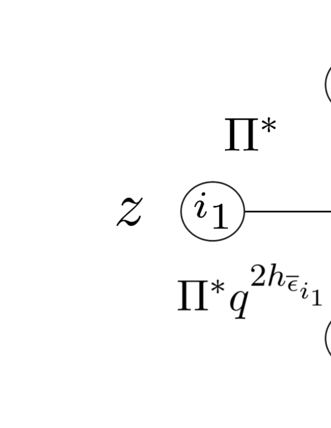
Let $(\pi_{w},\widehat{V}_{w})$ be the vector representation of $U_{q,p}(\widehat{{\mathfrak{gl}}}_{N})$ with $\widehat{V}=\bigoplus_{\mu=1}^{N}{\mathbb{F}}v_{\mu}$ and $\widehat{V}_{w}=\widehat{V}[w,w^{-1}]$ . See [22], B.2. We assume $e^{Q_{\alpha}}v_{\mu}=v_{\mu}$ ( $\alpha\in\overline{\mathfrak{H}}^{*}$ ). The action of the $L$ -operator ${L}^{+}(z)$ on $\widehat{V}_{w}$ is given by

\displaystyle\displaystyle\pi_{w}(L_{ij}^{+}(z))v_{\nu}=\pi_{w}(L_{ij}^{+}(z,\Pi^{*}))e^{-Q_{\overline{\epsilon}_{j}}}v_{\nu}=\sum_{\mu=1}^{N}

\displaystyle{{\widetilde{R}}}(z/w,\Pi^{*})_{i\mu}^{j\nu}v_{\mu}

(6.13)

where we take

\displaystyle{\widetilde{R}}(z,\Pi^{*})=a(z){{\overline{R}}}(z,\Pi^{*})

(6.14)

with $a(z)=\theta(q^{2}z)$ . See Figure 6.1. Then the action of $L^{+}(z)$ on $\widehat{V}_{z}\widetilde{\otimes}\widehat{V}_{w_{1}}\widetilde{\otimes}\cdots\widetilde{\otimes}\widehat{V}_{w_{n}}$ is given by the following ([24], Proposition 4.1).

Proposition 6.2.

		$\displaystyle(\pi_{w_{1}}\otimes\cdots\otimes\pi_{w_{n}})\Delta^{\prime(n-1)}(L^{+}(z))$
	$\displaystyle=$	$\displaystyle\overline{R}^{+(0n)}(z/w_{n},\Pi^{}q^{2\sum_{j=1}^{n-1}h^{(j)}})\overline{R}^{+(0n-1)}(z/w_{n-1},\Pi^{}q^{2\sum_{j=1}^{n-2}h^{(j)}})\cdots\overline{R}^{+(01)}(z/w_{1},\Pi^{*}).$		(6.15)

Here $\Delta^{\prime}$ denotes the opposite comultiplication of $\Delta$ in Sec.2.8.

For brevity, we denote $(\pi_{w_{1}}\otimes\cdots\otimes\pi_{w_{n}})\Delta^{\prime(n-1)}(L^{+}(z))$ by $L^{+}(z)$ . We set

\displaystyle L^{+}(z)=\sum_{k,l=1}^{N}E_{k,l}\widetilde{\otimes}L^{+}_{kl}(z)

with $L^{+}_{ij}(z)\in\operatorname{End}_{\mathbb{F}}(\widehat{V}_{w_{1}}\widetilde{\otimes}\cdots\widetilde{\otimes}\widehat{V}_{w_{n}})$ .

Refer to caption — Figure 6.1: Graphical description of the matrix elements ${\widetilde{R}}(z/w,\Pi^{*})_{i_{1}i_{2}}^{j_{1}j_{2}}$ .

Now let us consider the action of $L^{+}_{kl}(z)$ on the standard basis of $\widehat{V}_{w_{1}}\widetilde{\otimes}\cdots\widetilde{\otimes}\widehat{V}_{w_{n}}$ i.e. $\{v_{{\boldsymbol{\mu}}}:=v_{\mu_{1}}\widetilde{\otimes}\cdots\widetilde{\otimes}v_{\mu_{n}}\ |\ {\boldsymbol{\mu}}=({\mu_{1}},\dots,{\mu_{n}})\in[1,N]^{n}\ \}$ . We then set for ${\boldsymbol{\alpha}}\in[1,N]^{n}$

\displaystyle\displaystyle L^{+}_{kl}(z)\cdot v_{\boldsymbol{\alpha}}=\sum_{\boldsymbol{\beta}\in[1,N]^{n}}T_{kl}^{+}(z;w_{1},\dots,w_{n};\Pi^{*})_{\boldsymbol{\beta}}^{\boldsymbol{\alpha}}v_{\boldsymbol{\beta}}.

(6.16)

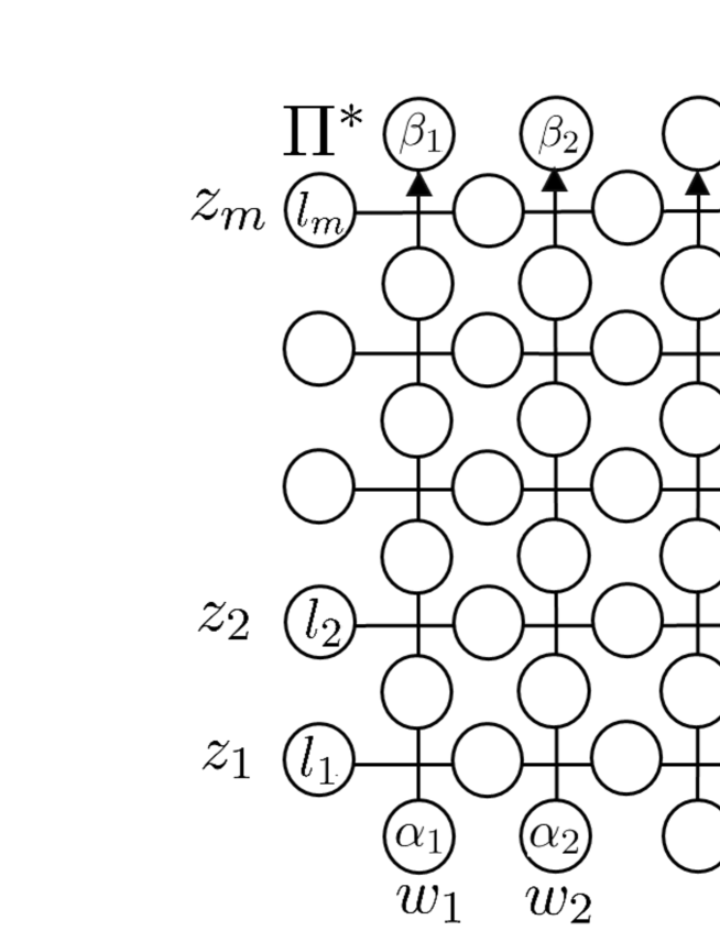
Making this action repeatedly, one obtains

		$\displaystyle L^{+}_{k_{m}l_{m}}(z_{m})L^{+}_{k_{m-1}l_{m-1}}(z_{m-1})\cdots L^{+}_{k_{1}l_{1}}(z_{1})v_{\boldsymbol{\alpha}}$
	$\displaystyle=$	$\displaystyle\sum_{\boldsymbol{\beta}\in[1,N]^{n}}Z_{{\bf K}\boldsymbol{\beta}}^{{\bf L}\boldsymbol{\alpha}}(z_{1},\dots,z_{m};w_{1},\dots,w_{n};\Pi^{*})v_{\boldsymbol{\beta}}$		(6.17)

with

	$\displaystyle Z_{{\bf K}\boldsymbol{\beta}}^{{\bf L}\boldsymbol{\alpha}}(z_{1},\dots,z_{m};w_{1},\dots,w_{n};\Pi^{*})$
$\displaystyle=$	$\displaystyle\sum_{\boldsymbol{\alpha}_{1},\dots,\boldsymbol{\alpha}_{m-1}\in[1,N]^{n}}T_{k_{m}l_{m}}^{+}(z_{m};z_{1},\dots,z_{n};\Pi^{})_{\boldsymbol{\beta}}^{\boldsymbol{\alpha}_{m-1}}T_{k_{m-1}l_{m-1}}^{+}(z_{m-1};w_{1},\dots,w_{n};\Pi^{}q^{2\langle\bar{\epsilon}_{l_{m}},h\rangle})_{\boldsymbol{\alpha}_{m-1}}^{\boldsymbol{\alpha}_{m-2}}\cdots$
	$\displaystyle\qquad\qquad\cdots T_{k_{1}l_{1}}^{+}(z_{1};w_{1},\dots,w_{n};\Pi^{*}q^{2\sum_{i=2}^{m}\langle\bar{\epsilon}_{l_{i}},h\rangle})_{\boldsymbol{\alpha}_{1}}^{\boldsymbol{\alpha}},$	(6.18)

where ${\bf K}=(k_{1},\dots,k_{m})$ , ${\bf L}=(l_{1},\dots,l_{m})$ , $\boldsymbol{\alpha}=(\alpha_{1},\dots,\alpha_{n})$ , $\boldsymbol{\beta}=(\beta_{1},\dots,\beta_{n})\in[1,N]^{n}$ . Note that from (6.15) each coefficient $Z_{{\bf K}{\boldsymbol{\beta}}}^{{\bf L}{\boldsymbol{\alpha}}}$ is given as a product of $R$ -matrices ${\widetilde{R}}^{+}(z,\Pi^{*})$ with the dynamical shifts. See Figure 6.2. The dynamical parameters in the matrix element ${\widetilde{R}}^{+}(z,\Pi^{*}q^{2\langle\bar{\epsilon}_{a},h\rangle})_{ij}^{kl}$ should be treated as $\Pi^{*}_{i,j}q^{2\langle\bar{\epsilon}_{a},h_{i,j}\rangle}=\Pi^{*}_{i,j}q^{2(\delta_{a,i}-\delta_{a,j})}$ .

6.2 The Gelfand-Tsetlin bases for $\widehat{V}_{w_{1}}\widetilde{\otimes}\cdots\widetilde{\otimes}\widehat{V}_{w_{n}}$

Let us consider ${\cal V}=\widehat{V}_{w_{1}}\widetilde{\otimes}\cdots\widetilde{\otimes}\widehat{V}_{w_{n}}$ with generic evaluation parameters $w_{1},\cdots,w_{n}$ . By the action (6.15), ${\cal V}$ is a $N^{n}$ -dimensional irreducible representation of $U_{q,p}(\widehat{{\mathfrak{gl}}}_{N})$ . It is the highest weight representation with the highest vector $\zeta=v_{(1^{n})}$ . Here $(1^{n})=(1,\cdots,1)$ . Using Proposition 6.2, we can check

\displaystyle\displaystyle L_{11}^{+}(z)\cdot\zeta=\prod_{l=1}^{n}a(z/w_{l})\zeta=\prod_{l=1}^{n}\theta(q^{2}z/w_{l})\zeta,

(6.19)

and

\displaystyle\displaystyle L_{ii}^{+}(z)\cdot\zeta=\prod_{l=1}^{n}a(z/w_{l})\overline{b}(z/w_{l})\zeta=\prod_{l=1}^{n}\theta(z/w_{l})\zeta,

(6.20)

for $i=2,\dots,N$ , hence the highest weight $\lambda(z)=(\lambda_{1}(z),\dots,\lambda_{N}(z))$ is given by

	$\displaystyle\lambda_{1}(z)$	$\displaystyle=\prod_{l=1}^{n}\theta(q^{2}z/w_{l}),$		(6.21)
	$\displaystyle\lambda_{i}(z)$	$\displaystyle=\prod_{l=1}^{n}\theta(z/w_{l}),\ \ \ i=2,\dots,N.$		(6.22)

In order to describe the Gelfand-Tsetlin bases, let us introduce a partition $I=(I_{1},\dots,I_{N})$ of $[1,n]=\{1,\dots,n\}$ , i.e.

\displaystyle I_{1}\cup\cdots\cup I_{N}=[1,n],\ \ \ I_{k}\cap I_{l}=\phi\ (k\neq l).

(6.23)

Let ${\cal I}_{n}$ be a set of all partitions of $[1,n]$ . For ${\boldsymbol{\mu}}=(\mu_{1},\mu_{2},\dots,\mu_{n})\in[1,N]^{n}$ , we define $I_{l}=\{i\in[1,n]\ |\ \mu_{i}=l\}$ ( $l=1,\dots,N$ ). Then $I=(I_{1},\dots,I_{N})\in{\cal I}_{n}$ . We often write thus obtained $I$ as $I=I_{\boldsymbol{\mu}}$ , and the corresponding standard base as $v_{I}=v_{\boldsymbol{\mu}}=v_{\mu_{1}}\widetilde{\otimes}\cdots\widetilde{\otimes}v_{\mu_{n}}$ .

In addition, for an index set $S=\{i_{1},i_{2},\dots,i_{r}\}$ with $i_{1}<i_{2}<\dots<i_{r}$ and the $L$ -operators $L^{+}_{kl}(z_{i_{a}})$ $(i_{a}\in S)$ , we write

\displaystyle L^{+}_{kl}(z_{S}):=\prod_{j\in S}^{\curvearrowleft}L^{+}_{kl}(z_{j})=L^{+}_{kl}(z_{i_{r}})\cdots L^{+}_{kl}(z_{i_{2}})L^{+}_{kl}(z_{i_{1}}).

Now we construct the Gelfand-Tsetlin bases in terms of the $L$ -operators.

Definition 6.2.

For $I\in{\cal I}_{n}$ , let us define a vector $\widetilde{\xi}_{I}\in{\cal V}$ by

\displaystyle\widetilde{\xi}_{I}=L_{N-1,N}^{+}(w_{I_{N}})L_{N-2,N-1}^{+}(w_{I_{N-1}\cup I_{N}})\cdots L_{12}^{+}(w_{I_{2}\cup\cdots\cup I_{N}})\cdot\zeta.

(6.24)

Example. Consider the case $N=3$ , $n=9$ , $I=I_{231213231}$ . Then $I_{1}=\{3<5<9\}$ , $I_{2}=\{1<4<7\}$ , $I_{3}=\{2<6<8\}$ . We have

	$\displaystyle\widetilde{\xi}_{I}$	$\displaystyle=L_{23}^{+}(w_{I_{3}})L_{12}^{+}(w_{I_{2}\cup I_{3}})\cdot\zeta$
		$\displaystyle=L_{23}^{+}(w_{8})L_{23}^{+}(w_{6})L_{23}^{+}(w_{2})L_{12}^{+}(w_{8})L_{12}^{+}(w_{7})L_{12}^{+}(w_{6})L_{12}^{+}(w_{4})L_{12}^{+}(w_{2})L_{12}^{+}(w_{1})\cdot\zeta.$		(6.25)

We show that the set of vectors $\{\widetilde{\xi}_{I}\}_{I\in{\cal I}_{n}}$ forms a basis of ${\cal V}$ , on which all the generators $A_{\ell}(z)$ of the Gelfand-Tsetlin subalgebras of $E_{q,p}(\widehat{\mathfrak{gl}}_{N})$ are simultaneously diagonalized.

Proposition 6.3.

The vector $\widetilde{\xi}_{I}$ is an eigenvector of $A_{l}(z)$ , $l=1,\dots,N$

\displaystyle A_{l}(z)\cdot\widetilde{\xi}_{I}=\prod_{k=1}^{N-l+1}\lambda_{N-l+1,k}^{I}(q^{-2k+2}z)\widetilde{\xi}_{I},

(6.26)

where $\lambda_{jk}^{I}(z)$ , $1\leq k\leq j\leq N$ are given by

	$\displaystyle\lambda_{j1}^{I}(z)$	$\displaystyle=\prod_{m=1}^{n}\theta(q^{2\delta_{m\in I_{N-j+1}\cup\cdots\cup I_{N}}}z/w_{m}),$		(6.27)
	$\displaystyle\lambda_{jk}^{I}(z)$	$\displaystyle=\prod_{m=1}^{n}\theta(z/w_{m}),\ \ \ k\neq 1.$		(6.28)

Here

\displaystyle\delta_{s\in S}=\left\{\begin{matrix}1&\ (s\in S)\cr 0&\ (s\not\in S)\cr\end{matrix}\right.

for any index set $S$ .

Proof.

Define $\widetilde{\xi}_{I}^{(l)}$ as

\displaystyle\widetilde{\xi}_{I}^{(l)}:=L_{N-l,N-l+1}^{+}(w_{I_{N-l+1}\cup\cdots\cup I_{N}})L_{N-l-1,N-l}^{+}(w_{I_{N-l}\cup\cdots\cup I_{N}})\cdots L_{12}^{+}(w_{I_{2}\cup\cdots\cup I_{N}})\cdot\zeta.

(6.29)

Then $\widetilde{\xi}_{I}$ can be expressed as

\displaystyle\widetilde{\xi}_{I}=L_{N-1,N}^{+}(w_{I_{N}})\cdots L_{l,l+1}^{+}(w_{I_{l+1}\cup\cdots\cup I_{N}})\cdot\widetilde{\xi}_{I}^{(N-l+1)}.

(6.30)

We first examine the action of $A_{l}(z)$ on $\widetilde{\xi}_{I}^{(N-l+1)}$ . By applying Lemma 6.1 repeatedly, one finds that $\widetilde{\xi}_{I}^{(N-l+1)}$ is a singular vector of weight $(\lambda_{N-l+1,1}^{I}(z),\lambda_{N-l+1,2}^{I}(z),\cdots,\lambda_{N-l+1,N-l+1}^{I}(z))$ with respect to the subalgebra $E_{q,p}(\widehat{{\mathfrak{gl}}}_{N-l+1})$ . Note $\lambda_{Nk}^{I}(z)=\lambda_{k}(z)$ , $k=1,\dots,N$ , where $(\lambda_{1}(z),\lambda_{2}(z),\dots,\lambda_{N}(z))$ is the weight for the highest vector $\widetilde{\xi}_{I}^{(N)}=\zeta$ . Since $\widetilde{\xi}_{I}^{(N-l+1)}$ is a singular vector, we have

	$\displaystyle L^{+}_{ij}(z)\cdot\widetilde{\xi}_{I}^{(N-l+1)}$	$\displaystyle=0,\ \ \qquad l\leq j<i\leq N,$		(6.31)
	$\displaystyle L^{+}_{l+k-1,l+k-1}(z)\cdot\widetilde{\xi}_{I}^{(N-l+1)}$	$\displaystyle=\lambda_{N-l+1,k}^{I}(z)\widetilde{\xi}_{I}^{(N-l+1)},\ \ \qquad k=1,\dots,N-l+1,$		(6.32)

From (2.83), we have

\displaystyle A_{l}(z)=\sum_{\sigma\in\mathfrak{S}_{N-l+1}}\mathrm{sgn}_{{[}l,N{]}}^{*}(\sigma,\Pi^{*})L^{+}_{l\sigma(l)}(z)L^{+}_{l+1\sigma(l+1)}(q^{-2}z)\cdots L^{+}_{N,\sigma(N)}(q^{-2N+2l}z).

(6.33)

Using (6.31), (6.32) and (6.33), we find that $\widetilde{\xi}_{I}^{(N-l+1)}$ is an eigenvector of $A_{l}(z)$ :

\displaystyle A_{l}(z)\cdot\widetilde{\xi}_{I}^{(N-l+1)}=\prod_{k=1}^{N-l+1}\lambda_{N-l+1,k}^{I}(q^{-2k+2}z)\widetilde{\xi}_{I}^{(N-l+1)}.

(6.34)

Next, we consider the action of $A_{l}(z)$ on $\widetilde{\xi}_{I}$ . Recall $A_{l}(z)$ is the center of the subalgebra $E_{q,p}(\widehat{{\mathfrak{gl}}}_{N-l+1})$ generated by $L^{+}_{ij}(w),\ l\leq i,j\leq N$

\displaystyle[A_{l}(z),L^{+}_{ij}(w)]=0,\ \ \ l\leq i,j\leq N.

(6.35)

Using (6.30), (6.34) and (6.35), we find that $\widetilde{\xi}_{I}$ is an eigenvector of $A_{l}(u)$ :

$\displaystyle A_{l}(z)\cdot\widetilde{\xi}_{I}$	$\displaystyle=A_{l}(z)L_{N-1,N}^{+}(w_{I_{N}})\cdots L_{l,l+1}^{+}(w_{I_{l+1}\cup\cdots\cup I_{N}})\cdot\widetilde{\xi}_{I}^{(N-l+1)}$
	$\displaystyle=L_{N-1,N}^{+}(w_{I_{N}})\cdots L_{l,l+1}^{+}(w_{I_{l+1}\cup\cdots\cup I_{N}})A_{l}(z)\cdot\widetilde{\xi}_{I}^{(N-l+1)}$
	$\displaystyle=\prod_{k=1}^{N-l+1}\lambda_{N-l+1,k}^{I}(q^{-2k+2}z)L_{N-1,N}^{+}(w_{I_{N}})\cdots L_{l,l+1}^{+}(w_{I_{l+1}\cup\cdots\cup I_{N}})\cdot\widetilde{\xi}_{I}^{(N-l+1)}$
	$\displaystyle=\prod_{k=1}^{N-l+1}\lambda_{N-l+1,k}^{I}(q^{-2k+2}z)\widetilde{\xi}_{I}.$	(6.36)

∎

Theorem 6.3.

The set of vectors $\{\widetilde{\xi}_{I}\}_{I\in{\cal I}_{n}}$ forms a basis of ${\cal V}$ .

Proof.

From Proposition 6.3, each vector $\widetilde{\xi}_{I}$ belongs to the different simultaneous eigenvalues of $A_{l}(z)$ $(1\leq l\leq N)$ so that $\widetilde{\xi}_{I}\ {(I\in{\cal I}_{n})}$ are linearly independent. The number of these vectors is

\displaystyle\sum_{(|I_{1}|,\cdots,|I_{N}|)\in{\mathbb{N}}^{N}\atop\sum_{a=1}^{N}|I_{a}|=n}\frac{n!}{|I_{1}|!\cdots|I_{N}|!}=N^{n}.

∎

In [24], the Gelfand-Tsetlin bases of ${\cal V}$ was constructed in a different way. Let us denote them by $\xi_{I}^{\prime}$ $(I\in{\cal I}_{n})$ . The construction is as follows. Let us define $\widetilde{S}_{i}(\Pi^{*})$ by

\displaystyle\widetilde{S}_{i}(\Pi^{*}):={\cal P}^{(ii+1)}{\overline{R}}^{(ii+1)}(z_{i}/z_{i+1},\Pi^{*}q^{2{\sum_{j=1}^{i-1}h^{(j)}}})s^{z}_{i},

where ${\cal P}$ and $s^{z}_{i}$ are the following permutation operators

\displaystyle{\cal P}:v\widetilde{\otimes}w\mapsto w\widetilde{\otimes}v,\qquad s^{z}_{i}f(\cdots,z_{i},z_{i+1},\cdots)=f(\cdots,z_{i+1},z_{i},\cdots)

for any function $f(z_{1},\cdots,z_{n})$ . Then by using the dynamical Yang-Baxter equation (2.15) and the unitarity relation for ${\overline{R}}(z,\Pi^{*})$ one can show the following.

Proposition 6.4.

	$\displaystyle\widetilde{S}_{i}(\Pi^{})\widetilde{S}_{i+1}(\Pi^{})\widetilde{S}_{i}(\Pi^{})=\widetilde{S}_{i+1}(\Pi^{})\widetilde{S}_{i}(\Pi^{})\widetilde{S}_{i+1}(\Pi^{}),$
	$\displaystyle\widetilde{S}_{i}(\Pi^{})\widetilde{S}_{j}(\Pi^{})=\widetilde{S}_{j}(\Pi^{})\widetilde{S}_{i}(\Pi^{})\qquad\qquad(\|i-j\|>1)$
	$\displaystyle\widetilde{S}_{i}(\Pi^{*})^{2}=1.$

For $I,J\in{\cal I}_{n}$ with $|I_{l}|=|J_{l}|$ $(l=1,\cdots,N)$ , let $I^{(l)}=\{i^{(l)}_{1}<\cdots<i^{(l)}_{\lambda^{(l)}}\}$ and $J^{(l)}=\{j^{(l)}_{1}<\cdots<j^{(l)}_{\lambda^{(l)}}\}$ $(l=1,\cdots,N)$ . We define a partial ordering $\leqslant$ by

\displaystyle I\leqslant J\Leftrightarrow i^{(l)}_{a}\leq j^{(l)}_{a}\qquad\forall l,a.

One then can construct the Gelfand-Tsetlin bases $\xi^{\prime}_{I}$ $(I\in{\cal I}_{n})$ by

\displaystyle\xi^{\prime}_{I^{max}}:=v_{I^{max}},\qquad\xi^{\prime}_{s_{i}(I)}:=\widetilde{S}_{i}(\Pi^{*})\xi_{I},

(6.37)

where $s_{i}(I)=I_{\cdots,\mu_{i+1},\mu_{i},\cdots}$ for $I=I_{\cdots,\mu_{i},\mu_{i+1},\cdots}$ , and

\displaystyle I^{max}=I_{\tiny\underbrace{N\cdots N}_{|I_{N}|}\ \cdots\underbrace{1\cdots 1}_{|I_{1}|}}.

In [24], the level-0 action of the Drinfeld generators on $\xi_{I}^{\prime}$ was explicitly obtained. In particular the $K^{+}_{l}(z)$ $(1\leq l\leq N)$ are simultaneously diagonalized as

\displaystyle\displaystyle K^{+}_{j}(z)\cdot\xi_{I}^{\prime}

\displaystyle=\prod_{m=1}^{n}\theta(q^{2}z/w_{m})\prod_{k=1}^{j-1}\prod_{a\in I_{k}}\frac{\theta(z/w_{a})}{\theta(q^{2}z/w_{a})}\prod_{l=j+1}^{N}\prod_{b\in I_{l}}\frac{\theta(q^{-2}z/w_{b})}{\theta(z/w_{b})}\xi_{I}^{\prime}.

(6.38)

Here we modified the formula obtained in [24] by considering the difference of the vector representations of $L^{+}(z)$ used there and in this section: in [24] it is defined by the $R$ -matrix ${{\overline{R}}}(z/w,\Pi^{*})$ (2.11) instead of ${\widetilde{R}}(z/w,\Pi^{*})=a(z/w){{\overline{R}}}(z/w,\Pi^{*})$ (6.14). One can rewrite this as

\displaystyle\displaystyle K^{+}_{j}(z)\cdot\xi_{I}^{\prime}

\displaystyle=\frac{\prod_{m=1}^{n}\theta(q^{2\delta_{m\in I_{j}\cup\cdots\cup I_{N}}}z/w_{m})\prod_{m=1}^{n}\theta(q^{-2}z/w_{m})}{\prod_{m=1}^{n}\theta(q^{2\delta_{m\in I_{j+1}\cup\cdots\cup I_{N}}-2}z/w_{m})}\xi_{I}^{\prime}.

(6.39)

Hence we have

	$\displaystyle A_{l}(z)\cdot\xi_{I}^{\prime}$	$\displaystyle=K^{+}_{l}(z)K^{+}_{l+1}(q^{-2}z)\cdots K^{+}_{N}(q^{-2N+2l}z)\cdot\xi_{I}^{\prime}$
		$\displaystyle=\prod_{m=1}^{n}\theta(q^{2\delta_{m\in I_{j}\cup\cdots\cup I_{N}}}z/w_{m})\prod_{m=1}^{n}\prod_{l=1}^{N-j}\theta(q^{-2l}z/w_{m})\xi_{I}^{\prime},$		(6.40)

which is in agreement with (6.26). Therefore the difference between $\widetilde{\xi}_{I}$ and $\xi_{I}^{\prime}$ is a multiplication by a scalar function. We determine this scalar function in Sec.6.4

6.3 Relation between $\xi_{\boldsymbol{\nu}}$ and $\widetilde{\xi}_{I}$

Let us compare the Gelfand-Tsetlin bases $\xi_{{\boldsymbol{\nu}}}$ ’s (5.15) in the previous section with $\widetilde{\xi}_{I}$ ’s (6.24). First, let us specialize the construction in the previous subsection to the tensor product of the vector representations. This means we restrict the tuples of Gelfand-Tsetlin patterns ${\boldsymbol{\lambda}}=({\boldsymbol{\lambda}}^{(1)},\dots,{\boldsymbol{\lambda}}^{(n)})$ to those labelled by $I$ . By comparing the eigenvalues of $A_{l}(z)$ (also recall $\overline{A}_{N+1-l}(z)=A_{l}(z)$ ), we find the following correspondence: $a^{(s)}=w_{s}$ , and

	$\displaystyle\lambda_{j,1}^{(s)}=\delta_{s\in I_{N-j+1}\cup\cdots\cup I_{N}},$
	$\displaystyle\lambda_{j,k}^{(s)}=0,\qquad k\neq j\qquad$

for $j=1,\dots,N$ . In terms of ${\boldsymbol{\nu}}=({\boldsymbol{\nu}}^{(1)},\dots,{\boldsymbol{\nu}}^{(n)})$ , the correspondence is

	$\displaystyle\nu_{j,j}^{(s)}=\delta_{s\in I_{N-j+1}\cup\cdots\cup I_{N}},$
	$\displaystyle\nu_{j,k}^{(s)}=0,\qquad k=1,\dots,j-1$

for $j=1,\dots,N$ . Then the $\overline{B}_{\ell}$ -operators which contribute to the product in (5.15) are only those specified by $(\ell,j,s)$ satisfying $\ell=j$ , $\nu^{(s)}_{j,j}=\delta_{s\in I_{N-j+1}\cup\cdots\cup I_{N}}=1$ , i.e. $\overline{B}_{j}(w_{s})$ $(1\leq j\leq N-1)$ with $s\in I_{N-j+1}\cup\cdots\cup I_{N}$ . Let us denote this $\xi_{{\boldsymbol{\nu}}}$ by ${\xi}_{I}$ . Noting $\overline{B}_{j}(w)=B_{N+1-j}(w)=\ell^{+}(w)_{\{N-j,N-j+2,\dots,N\}}^{[N+1-j,N]}$ , we have

\displaystyle{\xi}_{I}=\ell^{+}(w_{I_{N}})_{\{N-1\}}^{\{N\}}\ell^{+}(w_{I_{N-1}\cup I_{N}})_{\{N-2,N\}}^{[N-1,N]}\cdots\ell^{+}(w_{I_{2}\cup\cdots\cup I_{N}})_{\{1,3,\dots,N\}}^{[2,N]}\cdot\zeta.

(6.41)

Let us derive the scalar coefficient which relates ${\xi}_{I}$ (6.41) and $\widetilde{\xi}_{I}$ (6.24). We first show the following.

Proposition 6.4.

Let $I$ and $J$ be two partitions of $[1,n]$ such that $I_{l+2}=\cdots=I_{N}=\phi$ , $J_{l+2}=\cdots=J_{N}=\phi$ , $J_{l}=I_{l}\cup\{k\}$ , $J_{l+1}=I_{l+1}\backslash\{k\}$ , $J_{j}=I_{j}\ (j\neq l,l+1)$ . We have

\displaystyle\displaystyle\ell^{+}(w_{k})_{\{l,l+2,\dots,N\}}^{[l+1,N]}\cdot\widetilde{\xi}_{J}=\prod_{j=1}^{n}\prod_{a=1}^{N-l-1}\theta(q^{-2a}w_{k}/w_{j})\widetilde{\xi}_{I}.

(6.42)

Proof.

Using (2.89), we have

\displaystyle\displaystyle\ell^{+}(w_{k})_{\{l,l+2,\dots,N\}}^{[l+1,N]}\cdot\widetilde{\xi}_{J}=\sum_{j=1}^{N-l}\prod_{1\leq a<j}\frac{\theta(q^{2}\Pi_{i_{j},i_{a}})}{\theta(\Pi_{i_{a},i_{j}})}\ell^{+}(q^{-2}w_{k})_{\{l,l+2,\dots,N\}\backslash\{i_{j}\}}^{[l+2,N]}L^{+}_{i_{j},l+1}(w_{k})\cdot\widetilde{\xi}_{J},

(6.43)

where $i_{1}=l$ , $i_{a}=l+a$ ( $a=2,\dots,N-l$ ). From $\displaystyle L_{ij}^{+}(z)\cdot\widetilde{\xi}_{J}=0$ , $l+1\leq j<i\leq N$ , we note that only the summand corresponding to $j=1$ in (6.43) survives. Noting also $L^{+}_{l,l+1}(w_{k})\cdot\widetilde{\xi}_{J}=\widetilde{\xi}_{I}$ , we get

\displaystyle\displaystyle\ell^{+}(w_{k})_{\{l,l+2,\dots,N\}}^{[l+1,N]}\cdot\widetilde{\xi}_{J}=\ell^{+}(q^{-2}w_{k})_{[l+2,N]}^{[l+2,N]}L^{+}_{l,l+1}(w_{k})\cdot\widetilde{\xi}_{J}=\ell^{+}(q^{-2}w_{k})_{[l+2,N]}^{[l+2,N]}\cdot\widetilde{\xi}_{I}.

(6.44)

Noting that our vector $\widetilde{\xi}_{I}$ here is $\widetilde{\xi}_{I}^{(N-l)}$ , one can evaluate the right hand side of (6.44) by using (2.83) and the following properties.

	$\displaystyle L^{+}_{ij}(z)\cdot\widetilde{\xi}_{I}$	$\displaystyle=0,\ \ \ l+1\leq j<i\leq N,$		(6.45)
	$\displaystyle L^{+}_{l+k,l+k}(z)\cdot\widetilde{\xi}_{I}$	$\displaystyle=\lambda_{N-l,k}^{I}(z)\widetilde{\xi}_{I},\ \ \ k=1,\dots,N-l.$		(6.46)

These are obtained by replacing $l$ in (6.31) and (6.32) by $l+1$ . Then the result is

	$\displaystyle\ell^{+}(q^{-2}w_{k})_{[l+2,N]}^{[l+2,N]}\cdot\widetilde{\xi}_{I}$
$\displaystyle=$	$\displaystyle\sum_{\sigma\in\mathfrak{S}_{N-l-1}}\mathrm{sgn}_{[\ell+2,N]}^{}(\sigma,\Pi^{})L^{+}_{l+2,\sigma(l+2)}(q^{-2}w_{k})L^{+}_{l+3,\sigma(l+3)}(q^{-4}w_{k})\cdots L^{+}_{N,\sigma(N)}(q^{-2N+2+2l}w_{k})\cdot\widetilde{\xi}_{I}$
$\displaystyle=$	$\displaystyle\lambda_{N-l,2}^{I}(q^{-2}w_{k})\lambda_{N-l,3}^{I}(q^{-4}w_{k})\cdots\lambda_{N-l,N-l}^{I}(q^{-2N+2+2l}w_{k})\widetilde{\xi}_{I}$
$\displaystyle=$	$\displaystyle\prod_{j=1}^{n}\prod_{a=1}^{N-l-1}\theta(q^{-2a}w_{k}/w_{j})\widetilde{\xi}_{I}.$	(6.47)

From (6.44) and (6.47), we get (6.42).

∎

From (6.42) and $L^{+}_{l,l+1}(w_{k})\cdot\widetilde{\xi}_{J}=\widetilde{\xi}_{I}$ , we have the following relation.

Proposition 6.5.

\displaystyle\displaystyle{\xi}_{I}=\prod_{j=1}^{n}\prod_{l=1}^{N-1}\prod_{a=1}^{N-l-1}\theta(q^{-2a}w_{I_{l+1}\cup\cdots\cup I_{N}}/w_{j})\widetilde{\xi}_{I}.

(6.48)

6.4 The change of basis matrix

Now let us make a connection between $\widetilde{\xi}_{I}$ and $\xi^{\prime}_{I}$ . As shown in Sec.6.2, their difference is a multiplication by a scalar function

\displaystyle\widetilde{\xi}_{I}=N({\bf w})\xi_{I}^{\prime}.

(6.49)

We determine a function $N({\bf w})$ of the evaluation parameters ${\bf w}=(w_{1},\cdots,w_{n})$ . As a byproduct we obtain an explicit formula for the partition function of the 2-dimensional square lattice model defined by the elliptic $R$ -matrix ${\widetilde{R}}(z,\Pi^{*})$ (6.14) in terms of the elliptic weight function.

For this purpose let us consider the change of basis matrix $(\widetilde{X}_{IJ})_{I,J\in{\cal I}_{n}}$ from the standard basis $\{v_{I}\}_{I\in{\cal I}_{n}}$ to the Gelfand-Tsetlin basis $\{\widetilde{\xi}_{I}\}_{I\in{\cal I}_{n}}$ .

\displaystyle\widetilde{\xi}_{I}=\sum_{J\in{\cal I}_{n}}\widetilde{X}_{IJ}v_{J}.

From (6.17) and (6.24) with $\zeta=v_{(1^{n})}$ , the matrix element $\widetilde{X}_{IJ}$ for $J=J_{{\boldsymbol{\mu}}}$ with ${\boldsymbol{\mu}}=(\mu_{1},\dots,\mu_{n})$ is given by

\displaystyle\widetilde{X}_{IJ}=Z_{{\bf K}\;{\boldsymbol{\mu}}}^{{\bf L}(1^{n})}(w_{I_{2}\cup\cdots\cup I_{N}},w_{I_{3}\cup\cdots\cup I_{N}},\dots,w_{I_{N}};w_{1},\dots,w_{n};\Pi^{*}),

(6.50)

where ${\bf K}=(1^{|I_{2}\cup\cdots\cup I_{N}|},2^{|I_{3}\cup\cdots\cup I_{N}|},\dots,(N-1)^{|I_{N}|})$ and ${\bf L}=(2^{|I_{2}\cup\cdots\cup I_{N}|},3^{|I_{3}\cup\cdots\cup I_{N}|},\dots,N^{|I_{N}|})$ .

As a statistical model, $\widetilde{X}_{IJ}$ is a partition function of the 2-dimensional $n\times n$ square lattice model defined by assigning the $R$ -matrix elements ${\widetilde{R}}(z_{i}/w_{j},\Pi^{*}q^{2h_{\bullet}})_{i_{1}i_{2}}^{j_{1}j_{2}}$ on the vertex at $(i,j)$ (Figure 6.1)⁴⁴4We count the row from the bottom to the top and the column from the left to the right. as statistical weights. Here $(z_{1},\cdots,z_{n})$ is taken as $(w_{I_{2}\cup\cdots\cup I_{N}},w_{I_{3}\cup\cdots\cup I_{N}},\dots,w_{I_{N}})$ . On each link, the overlapped indices of the neighbor $R$ -matrices are summed over $1,\cdots,N$ (Figure 6.2).

On the other hand, in [24] the change of basis matrix from $\{v_{I}\}$ to $\{\xi^{\prime}_{I}\}$ was obtained explicitly in terms of the elliptic weight functions. Let us recall them. Let us set $I^{(l)}:=I_{1}\cup\cdots\cup I_{l}$ and denote its elements as $I^{(l)}=\{i_{1}^{(l)}<\cdots<i_{\lambda^{(l)}}^{(l)}\}$ , where we set $\lambda_{l}=|I_{l}|$ and $\lambda^{(l)}:=\lambda_{1}+\cdots+\lambda_{l}$ . To each $i_{a}^{(l)}$ ( $l=1,\dots,N$ , $a=1,\dots,\lambda^{(l)}$ ), we associate a variable $t_{a}^{(l)}\equiv t(i_{a}^{(l)})$ with $t_{a}^{(N)}=w_{a}$ $(a=1,\dots,n)$ and set ${\bf t}=(t_{a}^{(l)})$ $(l=1,\dots,N,a=1,\dots,\lambda^{(l)})$ and ${\bf w}=(w_{a})$ $(a=1,\dots,n)$ . Then the elliptic weight functions [22, 24] are given by

$\displaystyle\widetilde{W}_{I}({\bf t},{\bf w},\Pi^{*})$	$\displaystyle=\mathrm{Sym}_{t^{(1)}}\cdots\mathrm{Sym}_{t^{(N-1)}}\widetilde{U}_{I}(t,w,\Pi^{*}),$	(6.51)
$\displaystyle\widetilde{U}_{I}(t,w,\Pi^{*})$	$\displaystyle=\prod_{l=1}^{N-1}\prod_{a=1}^{{\lambda}^{(l)}}\Bigg{(}\frac{\theta(q^{-2C_{\mu_{s},l+1}(s)}\Pi^{}_{\mu_{s},l+1}t_{b}^{(l+1)}/t_{a}^{(l)})\theta(q^{2})}{\theta(q^{2}t_{b}^{(l+1)}/t_{a}^{(l)})\theta(q^{-2C_{\mu_{s},l+1}(s)}\Pi^{}_{\mu_{s},l+1})}\Bigg{\|}_{i_{b}^{(l+1)}=i_{a}^{(l)}=s}$
	$\displaystyle\times\prod_{\begin{subarray}{c}b=1\\ i_{b}^{(l+1)}>i_{a}^{(l)}\end{subarray}}^{\lambda^{(l+1)}}\frac{\theta(t_{b}^{(l+1)}/t_{a}^{(l)})}{\theta(q^{2}t_{b}^{(l+1)}/t_{a}^{(l)})}\prod_{b=a+1}^{\lambda^{(l)}}\frac{\theta(q^{-2}t_{a}^{(l)}/t_{b}^{(l)})}{\theta(t_{a}^{(l)}/t_{b}^{(l)})}\Bigg{)},$	(6.52)

where we set $C_{\mu_{s},l+1}(s):=\sum_{j=s+1}^{n}\langle\overline{\epsilon}_{\mu_{j}},h_{\mu_{s},l+1}\rangle$ $(\mu_{s}\leq l)$ , and $\mathrm{Sym}_{t^{(l)}}$ denotes symmetrization over the variables $t_{1}^{(l)},\dots,t_{\lambda^{(l)}}^{(l)}$ .

Define the specialization ${\bf t}={\bf w}_{I}$ by $t_{a}^{(l)}=w_{i_{a}^{(l)}}(l=1,\dots,N-1,a=1,\dots,\lambda^{(l)})$ . One obtains the lower triangular matrix $X=(\widetilde{W}_{J}({\bf w}_{I},{\bf w},\Pi^{*}))_{I,J\in{\cal I}_{\lambda}}$ [22]. Here we put the matrix elements in the decreasing order $I^{max}\geqslant\cdots\geqslant I^{min}$ . For $\lambda=(\lambda_{1},\cdots,\lambda_{N})\in{\mathbb{N}}^{N}$ , $\mathcal{I}_{\lambda}$ denotes the set of all partition $I$ of $[1,n]$ satisfying $I_{l}=\lambda_{l}$ $l=1,\dots,N$ . Then one obtains the following statement.

Theorem 6.6.

([24] Thm 4.5)

\displaystyle\displaystyle\xi_{I}^{\prime}=\sum_{J\in\mathcal{I}_{\lambda}}\widetilde{W}_{J}({\bf w}_{I},{\bf w},\Pi^{*}q^{2\sum_{j=1}^{n}\langle\overline{\epsilon}_{\mu_{j}},h\rangle})v_{J}.

(6.53)

From (6.49) and the invertibility of the change of basis matrices, one obtains the following formula for the partition function.

Proposition 6.5.

\displaystyle Z_{{\bf K}\;{\boldsymbol{\mu}}}^{{\bf L}(1^{n})}(w_{I_{2}\cup\cdots\cup I_{N}},w_{I_{3}\cup\cdots\cup I_{N}},\dots,w_{I_{N}};{\bf w};\Pi^{*})=N({\bf w})\widetilde{W}_{J}({\bf w}_{I},{\bf w},\Pi^{*}q^{2\sum_{j=1}^{n}\langle\overline{\epsilon}_{\mu_{j}},h\rangle})

with $J=J_{{\boldsymbol{\mu}}}$ , ${\bf K}=(1^{|I_{2}\cup\cdots\cup I_{N}|},2^{|I_{3}\cup\cdots\cup I_{N}|},\dots,(N-1)^{|I_{N}|})$ and ${\bf L}=(2^{|I_{2}\cup\cdots\cup I_{N}|},3^{|I_{3}\cup\cdots\cup I_{N}|},\dots,N^{|I_{N}|})$ .

Example. The case of $N=2$ , $n=3$ , $\lambda=(2,1)$ : one has

$\displaystyle\displaystyle\widetilde{W}_{I_{211}}(w_{I_{112}},w,\Pi^{*})$	$\displaystyle=\frac{\theta(q^{-2}\Pi^{}_{1,2}w_{3}/w_{1})\theta(q^{2})}{\theta(q^{2}w_{3}/w_{1})\theta(q^{-2}\Pi^{}_{1,2})},$	(6.54)
$\displaystyle\displaystyle\widetilde{W}_{I_{121}}(w_{I_{112}},w,\Pi^{*})$	$\displaystyle=\frac{\theta(w_{3}/w_{1})\theta(\Pi^{}_{1,2}w_{3}/w_{2})\theta(q^{2})}{\theta(q^{2}w_{3}/w_{1})\theta(q^{2}w_{3}/w_{2})\theta(\Pi^{}_{1,2})},$	(6.55)
$\displaystyle\displaystyle\widetilde{W}_{I_{111}}(w_{I_{112}},w,\Pi^{*})$	$\displaystyle=\frac{\theta(w_{3}/w_{1})\theta(w_{3}/w_{2})}{\theta(q^{2}w_{3}/w_{1})\theta(q^{2}w_{3}/w_{2})},$	(6.56)

and

$\displaystyle\displaystyle\xi_{112}^{\prime}=$	$\displaystyle\displaystyle\widetilde{W}_{I_{211}}(w_{I_{112}},w,\Pi^{}q^{2<2\overline{\epsilon}_{1}+\overline{\epsilon}_{2},h>})v_{211}+\displaystyle\widetilde{W}_{I_{121}}(w_{I_{112}},w,\Pi^{}q^{2<2\overline{\epsilon}_{1}+\overline{\epsilon}_{2},h>})v_{121}$
	$\displaystyle+\displaystyle\widetilde{W}_{I_{111}}(w_{I_{112}},w,\Pi^{*}q^{2<2\overline{\epsilon}_{1}+\overline{\epsilon}_{2},h>})v_{111}$
$\displaystyle=$	$\displaystyle\frac{\theta(\Pi^{}_{1,2}w_{3}/w_{1})\theta(q^{2})}{\theta(q^{2}w_{3}/w_{1})\theta(\Pi^{}_{1,2})}v_{211}+\frac{\theta(w_{3}/w_{1})\theta(q^{2}\Pi^{}_{1,2}w_{3}/w_{2})\theta(q^{2})}{\theta(q^{2}w_{3}/w_{1})\theta(q^{2}w_{3}/w_{2})\theta(q^{2}\Pi^{}_{1,2})}v_{121}$
	$\displaystyle+\frac{\theta(w_{3}/w_{1})\theta(w_{3}/w_{2})}{\theta(q^{2}w_{3}/w_{1})\theta(q^{2}w_{3}/w_{2})}v_{112}.$	(6.57)

On the other hand, by direct computation, we find

	$\displaystyle\widetilde{\xi}_{112}=$	$\displaystyle\frac{\theta(\Pi^{}_{1,2}w_{3}/w_{1})\theta(q^{2})^{2}\theta(q^{2}w_{3}/w_{2})}{\theta(\Pi^{}_{1,2})}v_{211}+\frac{\theta(w_{3}/w_{1})\theta(q^{2}\Pi^{}_{1,2}w_{3}/w_{2})\theta(q^{2})^{2}}{\theta(q^{2}\Pi^{}_{1,2})}v_{121}$
		$\displaystyle+\theta(w_{3}/w_{1})\theta(w_{3}/w_{2})\theta(q^{2})v_{112}.$		(6.58)

The relation between $\widetilde{\xi}_{112}$ and $\xi_{112}^{\prime}$ is $\widetilde{\xi}_{112}=\theta(q^{2})\theta(q^{2}w_{3}/w_{2})\theta(q^{2}w_{3}/w_{1})\xi_{112}^{\prime}$ .

In the rest of this section, we determine $N({\bf w})$ as the ratio of the diagonal elements of $\widetilde{X}$ and $X$ . For $X$ , we have the result.

Proposition 6.7.

([22], Prop 5.1)

\displaystyle\widetilde{W}_{I}({\bf w}_{I},{\bf w},\Pi^{*})=\prod_{1\leq k<l<N}\prod_{a\in I_{k}}\prod_{\begin{subarray}{c}b\in I_{l}\\ a<b\end{subarray}}\frac{\theta(w_{b}/w_{a})}{\theta(q^{2}w_{b}/w_{a})}.

(6.59)

We show that the diagonal elements $\widetilde{X}_{II}$ can be calculated recursively and have a factored expression. To illustrate the calculation, let us show an example.

Example. Take $N=3$ , $n=9$ , $I=I_{231213231}$ . From the example in Sec.6.2, we have

$\displaystyle\widetilde{X}_{II}=$	$\displaystyle Z_{(1^{6},2^{3}),(231213231)}^{(2^{6},3^{3}),(1^{9})}(w_{1},w_{2},w_{4},w_{6},w_{7},w_{8},w_{2},w_{6},w_{8};w_{1},\dots,w_{9};\Pi^{*})$
$\displaystyle=$	$\displaystyle\sum_{\boldsymbol{\alpha}_{1},\dots,\boldsymbol{\alpha}_{8}\in[1,3]^{9}}T_{23}^{+}(w_{8};w_{1},\dots,w_{9};\Pi^{*})_{(231213231)}^{\boldsymbol{\alpha}_{8}}$
	$\displaystyle\times T_{23}^{+}(w_{6};w_{1},\dots,w_{9};\Pi^{}q^{2h_{\overline{\epsilon}_{3}}})_{\boldsymbol{\alpha}_{8}}^{\boldsymbol{\alpha}_{7}}T_{23}^{+}(w_{2};w_{1},\dots,w_{9};\Pi^{}q^{2h_{2\overline{\epsilon}_{3}}})_{\boldsymbol{\alpha}_{7}}^{\boldsymbol{\alpha}_{6}}$
	$\displaystyle\times T_{12}^{+}(w_{8};w_{1},\dots,w_{9};\Pi^{}q^{2h_{3\overline{\epsilon}_{3}}})_{\boldsymbol{\alpha}_{6}}^{\boldsymbol{\alpha}_{5}}T_{12}^{+}(w_{7};w_{1},\dots,w_{9};\Pi^{}q^{2h_{\overline{\epsilon}_{2}+3\overline{\epsilon}_{3}}})_{\boldsymbol{\alpha}_{5}}^{\boldsymbol{\alpha}_{4}}$
	$\displaystyle\times T_{12}^{+}(w_{6};w_{1},\dots,w_{9};\Pi^{}q^{2h_{2\overline{\epsilon}_{2}+3\overline{\epsilon}_{3}}})_{\boldsymbol{\alpha}_{4}}^{\boldsymbol{\alpha}_{3}}T_{12}^{+}(w_{4};w_{1},\dots,w_{9};\Pi^{}q^{2h_{3\overline{\epsilon}_{2}+3\overline{\epsilon}_{3}}})_{\boldsymbol{\alpha}_{3}}^{\boldsymbol{\alpha}_{2}}$
	$\displaystyle\times T_{12}^{+}(w_{2};w_{1},\dots,w_{9};\Pi^{}q^{2h_{4\overline{\epsilon}_{2}+3\overline{\epsilon}_{3}}})_{\boldsymbol{\alpha}_{2}}^{\boldsymbol{\alpha}_{1}}T_{12}^{+}(w_{1};w_{1},\dots,w_{9};\Pi^{}q^{2h_{5\overline{\epsilon}_{2}+3\overline{\epsilon}_{3}}})_{\boldsymbol{\alpha}_{1}}^{(1^{9})}.$	(6.60)

See Figure 6.3 for a graphical description of (6.60).

Taking $\boldsymbol{\alpha}_{j}=(\alpha_{j},\boldsymbol{\alpha}_{j}^{\prime})$ with $\alpha_{j}\in[1,3]$ and ${\boldsymbol{\alpha}}_{j}^{\prime}\in[1,3]^{8}$ , $j=1,\dots,8$ , we decompose (6.60) as

\displaystyle\sum_{\alpha_{1},\dots,\alpha_{8},\mu_{1},\dots,\mu_{9}\in[1,3]}C(\alpha_{1},\dots,\alpha_{8};\mu_{1},\dots,\mu_{9})Z(\alpha_{1},\dots,\alpha_{8};\mu_{1},\dots,\mu_{9}),

(6.61)

where we set

	$\displaystyle C(\alpha_{1},\dots,\alpha_{8};\mu_{1},\dots,\mu_{9})$
	$\displaystyle={\widetilde{R}}(w_{8}/w_{1},\Pi^{})_{\mu_{9}2}^{3\alpha_{8}}{\widetilde{R}}(w_{6}/w_{1},\Pi^{}q^{2h_{\overline{\epsilon}_{3}}})_{\mu_{8}\alpha_{8}}^{3\alpha_{7}}{\widetilde{R}}(w_{2}/w_{1},\Pi^{*}q^{2h_{2\overline{\epsilon}_{3}}})_{\mu_{7}\alpha_{7}}^{3\alpha_{6}}$
	$\displaystyle\times{\widetilde{R}}(w_{8}/w_{1},\Pi^{}q^{2h_{3\overline{\epsilon}_{3}}})_{\mu_{6}\alpha_{6}}^{2\alpha_{5}}{\widetilde{R}}(w_{7}/w_{1},\Pi^{}q^{2h_{\overline{\epsilon}_{2}+3\overline{\epsilon}_{3}}})_{\mu_{5}\alpha_{5}}^{2\alpha_{4}}$
	$\displaystyle\times{\widetilde{R}}(w_{6}/w_{1},\Pi^{}q^{2h_{2\overline{\epsilon}_{2}+3\overline{\epsilon}_{3}}})_{\mu_{4}\alpha_{4}}^{2\alpha_{3}}{\widetilde{R}}(w_{4}/w_{1},\Pi^{}q^{2h_{3\overline{\epsilon}_{2}+3\overline{\epsilon}_{3}}})_{\mu_{3}\alpha_{3}}^{2\alpha_{2}}$
	$\displaystyle\times{\widetilde{R}}(w_{2}/w_{1},\Pi^{}q^{2h_{4\overline{\epsilon}_{2}+3\overline{\epsilon}_{3}}})_{\mu_{2}\alpha_{2}}^{2\alpha_{1}}{\widetilde{R}}(w_{1}/w_{1},\Pi^{}q^{2h_{5\overline{\epsilon}_{2}+3\overline{\epsilon}_{3}}})_{\mu_{1}\alpha_{1}}^{21},$		(6.62)
	$\displaystyle Z(\alpha_{1},\dots,\alpha_{8};\mu_{1},\dots,\mu_{9})$
	$\displaystyle=\sum_{\boldsymbol{\alpha}_{1}^{\prime},\dots,\boldsymbol{\alpha}_{8}^{\prime}\in[1,3]^{8}}T_{2\mu_{9}}^{+}(w_{8};w_{2},\dots,w_{9};\Pi^{*}q^{2h_{\overline{\epsilon}_{2}}})_{(31213231)}^{\boldsymbol{\alpha}_{8}^{\prime}}$
	$\displaystyle\times T_{2\mu_{8}}^{+}(w_{6};w_{2},\dots,w_{9};\Pi^{}q^{2h_{\overline{\epsilon}_{3}+\overline{\epsilon}_{\alpha_{8}}}})_{\boldsymbol{\alpha}_{8}^{\prime}}^{\boldsymbol{\alpha}_{7}^{\prime}}T_{2\mu_{7}}^{+}(w_{2};w_{2},\dots,w_{9};\Pi^{}q^{2h_{2\overline{\epsilon}_{3}+\overline{\epsilon}_{\alpha_{7}}}})_{\boldsymbol{\alpha}_{7}^{\prime}}^{\boldsymbol{\alpha}_{6}^{\prime}}$
	$\displaystyle\times T_{1\mu_{6}}^{+}(w_{8};w_{2},\dots,w_{9};\Pi^{}q^{2h_{3\overline{\epsilon}_{3}+\overline{\epsilon}_{\alpha_{6}}}})_{\boldsymbol{\alpha}_{6}^{\prime}}^{\boldsymbol{\alpha}_{5}^{\prime}}T_{1\mu_{5}}^{+}(w_{7};w_{2},\dots,w_{9};\Pi^{}q^{2h_{\overline{\epsilon}_{2}+3\overline{\epsilon}_{3}+\overline{\epsilon}_{\alpha_{5}}}})_{\boldsymbol{\alpha}_{5}^{\prime}}^{\boldsymbol{\alpha}_{4}^{\prime}}$
	$\displaystyle\times T_{1\mu_{4}}^{+}(w_{6};w_{2},\dots,w_{9};\Pi^{}q^{2h_{2\overline{\epsilon}_{2}+3\overline{\epsilon}_{3}+\overline{\epsilon}_{\alpha_{4}}}})_{\boldsymbol{\alpha}_{4}^{\prime}}^{\boldsymbol{\alpha}_{3}^{\prime}}T_{1\mu_{3}}^{+}(w_{4};w_{2},\dots,w_{9};\Pi^{}q^{2h_{3\overline{\epsilon}_{2}+3\overline{\epsilon}_{3}+\overline{\epsilon}_{\alpha_{3}}}})_{\boldsymbol{\alpha}_{3}^{\prime}}^{\boldsymbol{\alpha}_{2}^{\prime}}$
	$\displaystyle\times T_{1\mu_{2}}^{+}(w_{2};w_{2},\dots,w_{9};\Pi^{}q^{2h_{4\overline{\epsilon}_{2}+3\overline{\epsilon}_{3}+\overline{\epsilon}_{\alpha_{2}}}})_{\boldsymbol{\alpha}_{2}^{\prime}}^{\boldsymbol{\alpha}_{1}^{\prime}}T_{1\mu_{1}}^{+}(w_{1};w_{2},\dots,w_{9};\Pi^{}q^{2h_{5\overline{\epsilon}_{2}+3\overline{\epsilon}_{3}+\overline{\epsilon}_{\alpha_{1}}}})_{\boldsymbol{\alpha}_{1}^{\prime}}^{(1^{8})}.$		(6.63)

The $C(\alpha_{1},\dots,\alpha_{8};\mu_{1},\dots,\mu_{9})$ part corresponds to the 1st column (the left most column ) in Figure 6.3. We now show that $\alpha_{1},\dots,\alpha_{8}$ , $\mu_{1},\dots,\mu_{9}$ in (6.61) are determined uniquely. In fact, applying the property

\displaystyle{{\widetilde{R}}}(z,P)_{kl}^{ij}=0\ \ \ \mathrm{unless}\ \ \ i=k,\ j=l\ \ \ \mathrm{or}\ \ \ i=l,\ j=k

(6.64)

to each factor in $C(\alpha_{1},\dots,\alpha_{8};\mu_{1},\dots,\mu_{9})$ , one finds

•

${\widetilde{R}}(w_{8}/w_{1},\Pi^{*})_{\mu_{9}2}^{3\alpha_{8}}$ yields $\alpha_{8}=2$ , $\mu_{9}=3$
•

${\widetilde{R}}(w_{6}/w_{1},\Pi^{*}q^{2h_{\overline{\epsilon}_{3}}})_{\mu_{8}\alpha_{8}}^{3\alpha_{7}}$ with $\alpha_{8}=2$ yields $\alpha_{7}=2$ , $\mu_{8}=3$
•

${{\widetilde{R}}}(w_{2}/w_{1},\Pi^{*}q^{2h_{2\overline{\epsilon}_{3}}})_{\mu_{7}\alpha_{7}}^{3\alpha_{6}}$ with $\alpha_{7}=2$ yields $\alpha_{6}=2$ , $\mu_{7}=3$ .
•

${\widetilde{R}}(w_{1}/w_{1},\Pi^{*}q^{2h_{5\overline{\epsilon}_{2}+3\overline{\epsilon}_{3}}})_{\mu_{1}\alpha_{1}}^{21}$ yields $\alpha_{1}=2$ , $\mu_{1}=1$ due to ${\widetilde{R}}(w_{1}/w_{1},\Pi^{*}q^{2h_{5\overline{\epsilon}_{2}+3\overline{\epsilon}_{3}}})_{21}^{21}=\theta(w_{1}/w_{1})=0$
•

the factors ${\widetilde{R}}(w_{2}/w_{1},\Pi^{*}q^{2h_{4\overline{\epsilon}_{2}+3\overline{\epsilon}_{3}}})_{\mu_{2}\alpha_{2}}^{2\alpha_{1}}$ , ${\widetilde{R}}(w_{4}/w_{1},\Pi^{*}q^{2h_{3\overline{\epsilon}_{2}+3\overline{\epsilon}_{3}}})_{\mu_{3}\alpha_{3}}^{2\alpha_{2}}$ , ${\widetilde{R}}(w_{6}/w_{1},\Pi^{*}q^{2h_{2\overline{\epsilon}_{2}+3\overline{\epsilon}_{3}}})_{\mu_{4}\alpha_{4}}^{2\alpha_{3}}$ ,
${\widetilde{R}}(w_{7}/w_{1},\Pi^{*}q^{2h_{\overline{\epsilon}_{2}+3\overline{\epsilon}_{3}}})_{\mu_{5}\alpha_{5}}^{2\alpha_{4}}$ and ${\widetilde{R}}(w_{8}/w_{1},\Pi^{*}q^{2h_{3\overline{\epsilon}_{3}}})_{\mu_{6}\alpha_{6}}^{2\alpha_{5}}$ in this order with $\alpha_{1}=2$ yield $\alpha_{2}=\cdots=\alpha_{6}=\mu_{2}=\cdots=\mu_{6}=2$ .

Therefore we obtain

\displaystyle\displaystyle\widetilde{X}_{II}=

\displaystyle C(2^{8};1,2^{5},3^{3})Z_{(1^{6},2^{3}),(31213231)}^{(1,2^{5},3^{3}),(1^{8})}(w_{1},w_{2},w_{4},w_{6},w_{7},w_{8},w_{2},w_{6},w_{8};w_{2},\dots,w_{9};\Pi^{*}q^{2h_{\overline{\epsilon}_{2}}}).

(6.65)

Here we made the identification

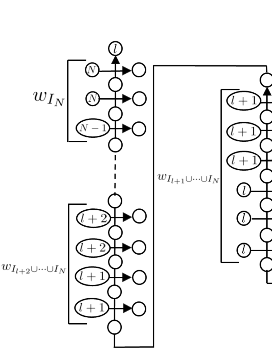
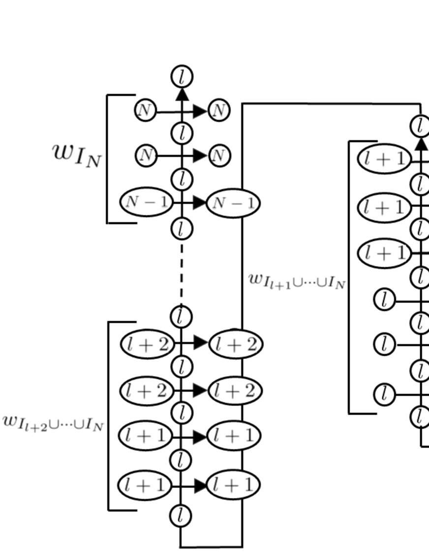
\displaystyle Z(2^{8};1,2^{5},3^{3})=Z_{(1^{6},2^{3}),(31213231)}^{(1,2^{5},3^{3}),(1^{8})}(w_{1},w_{2},w_{4},w_{6},w_{7},w_{8},w_{2},w_{6},w_{8};w_{2},\dots,w_{9};\Pi^{*}q^{2h_{\overline{\epsilon}_{2}}}).

We can repeat this process and find that $\widetilde{X}_{II}$ can be written as a product of the $R$ -matrix elements uniquely determined by the configuration at the boundary of the lattice (Figure 6.4). From the perspective of partition functions, this means that there is only one configuration which gives nonzero contribution.

Theorem 6.6.

	$\displaystyle\displaystyle\widetilde{X}_{II}=$	$\displaystyle\ \theta(q^{2})^{\sum_{k=2}^{N}(k-1)\|I_{k}\|}\prod_{l=1}^{N-1}\Bigg{\{}\prod_{\begin{subarray}{c}j\in I_{N-l+1}\cup\cdots\cup I_{N}\\ k\in I_{1}\cup\cdots\cup I_{N-l-1}\end{subarray}}\theta(w_{j}/w_{k})$
		$\displaystyle\times\prod_{\begin{subarray}{c}j\in I_{N-l+1}\cup\cdots\cup I_{N}\\ k\in I_{N-l}\cup\cdots\cup I_{N}\\ j<k\end{subarray}}\theta(q^{2}w_{j}/w_{k})\prod_{\begin{subarray}{c}j\in I_{N-l+1}\cup\cdots\cup I_{N}\\ k\in I_{N-l+1}\cup\cdots\cup I_{N}\\ j>k\end{subarray}}\theta(q^{2}w_{j}/w_{k})\prod_{\begin{subarray}{c}j\in I_{N-l+1}\cup\cdots\cup I_{N}\\ k\in I_{N-l}\\ j>k\end{subarray}}\theta(w_{j}/w_{k})\Bigg{\}}.$		(6.66)

Proof.

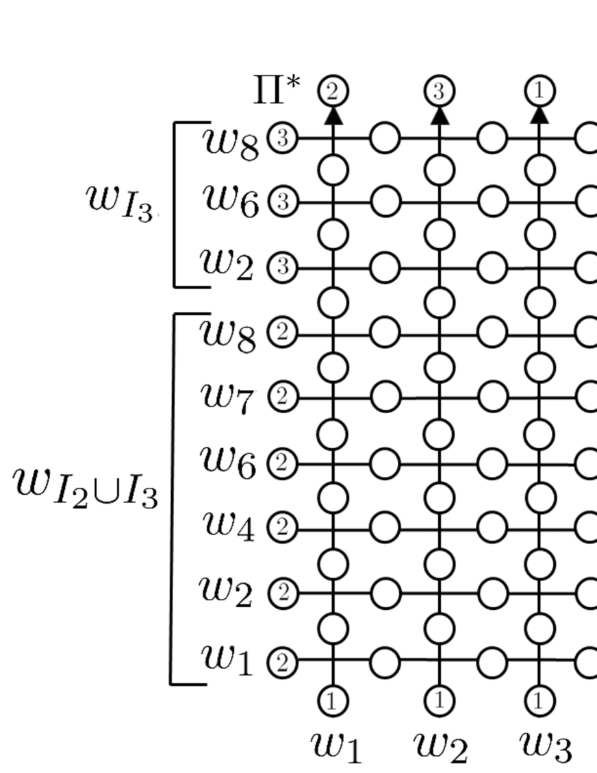
The diagonal matrix element $\widetilde{X}_{II}$ is given by (6.50) with $I=J_{{\boldsymbol{\mu}}}$ , ${\boldsymbol{\mu}}=(\mu_{1},\cdots,\mu_{n})$ . We show that $\widetilde{X}_{II}$ is factored into a product of the matrix elements of the $R$ -matrices determined uniquely by the boundary configuration.

To show this inductively in the number of columns in the lattice, let us introduce the following. For $k=1,\dots,n$ and $j=1,\cdots,N$ , let us set $n(I,k,j):=|\{\mu_{1},\dots,\mu_{k}\in I_{j}\}|$ and ${I_{j}\cup\cdots\cup I_{N}}=\{i_{1}^{[j,N]}<i_{2}^{[j,N]}<\cdots<i_{|I_{j}\cup\cdots\cup I_{N}|}^{[j,N]}\}$ . We define the $k$ -th partition function by

	$\displaystyle Z_{k}:=Z_{{\bf K}_{k}\;(\mu_{k},\dots,\mu_{n})}^{{\bf L}(1^{n+1-k})}(w_{i_{1}^{[2,N]}},\dots,w_{i_{\|I_{2}\cup\cdots\cup I_{N}\|}^{[2,N]}},w_{i_{1}^{[3,N]}},\dots,w_{i_{\|I_{3}\cup\cdots\cup I_{N}\|}^{[3,N]}},\dots,w_{i_{1}^{[N,N]}},\dots,w_{i_{\|I_{N}\|}^{[N,N]}};$
	$\displaystyle\qquad\qquad\qquad\qquad\qquad\qquad w_{k},\dots,w_{n};\Pi^{*}q^{\sum_{l=1}^{k-1}2h_{\overline{\epsilon}_{\mu_{l}}}}).$		(6.67)

Here, ${\bf K}_{k}=(1^{n(I,k,2)+\cdots+n(I,k,N)},2^{|I_{2}\cup\dots\cup I_{N}|-n(I,k,2)},3^{|I_{3}\cup\dots\cup I_{N}|-n(I,k,3)},\dots,N^{|I_{N}|-n(I,k,N)})$ , and we fix the order of the variables $(w_{I_{2}\cup\cdots\cup I_{N}},w_{I_{3}\cup\cdots\cup I_{N}},\dots,w_{I_{N}})$ as

\displaystyle(w_{i_{1}^{[2,N]}},\dots,w_{i_{|I_{2}\cup\cdots\cup I_{N}|}^{[2,N]}},w_{i_{1}^{[3,N]}},\dots,w_{i_{|I_{3}\cup\cdots\cup I_{N}|}^{[3,N]}},\dots,w_{i_{1}^{[N,N]}},\dots,w_{i_{|I_{N}|}^{[N,N]}}).

We show that from the $k$ -th partition function $Z_{k}$ one can obtain the $k+1$ -th partition $Z_{k+1}$ by removing the $k$ -th column as illustrated in the above example. The precise relation between $Z_{k}$ and $Z_{k+1}$ is given below. We also set $Z_{n+1}:=1$ .

Lemma 6.8.

For $k\in I_{l}$ , the relation between $Z_{k}$ and $Z_{k+1}$ is given by

\displaystyle Z_{k}=W_{k}Z_{k+1},

(6.68)

where

$\displaystyle W_{k}$	$\displaystyle=W_{k}^{1}W_{k}^{2}W_{k}^{3},$	(6.69)
$\displaystyle W_{k}^{1}$	$\displaystyle=\prod_{\begin{subarray}{c}j\in I_{N}\end{subarray}}\theta(w_{j}/w_{k})\prod_{\begin{subarray}{c}j\in I_{N-1}\cup I_{N}\end{subarray}}\theta(w_{j}/w_{k})\cdots\prod_{\begin{subarray}{c}j\in I_{l+2}\cup\cdots\cup I_{N}\end{subarray}}\theta(w_{j}/w_{k}),$	(6.70)
$\displaystyle W_{k}^{2}$	$\displaystyle=\prod_{\begin{subarray}{c}j\in I_{l+1}\cup\cdots\cup I_{N}\\ j>k\end{subarray}}\theta(w_{j}/w_{k})\prod_{\begin{subarray}{c}j\in I_{l+1}\cup\cdots\cup I_{N}\\ j<k\end{subarray}}\theta(q^{2}w_{j}/w_{k}),$	(6.71)
$\displaystyle W_{k}^{3}$	$\displaystyle=\Bigg{\{}\theta(q^{2})\prod_{\begin{subarray}{c}j\in I_{l}\cup\cdots\cup I_{N}\\ j>k\end{subarray}}\theta(q^{2}w_{j}/w_{k})\prod_{\begin{subarray}{c}j\in I_{l}\cup\cdots\cup I_{N}\\ j<k\end{subarray}}\theta(q^{2}w_{j}/w_{k})\Bigg{\}}$
	$\displaystyle\times\Bigg{\{}\theta(q^{2})\prod_{\begin{subarray}{c}j\in I_{l-1}\cup\cdots\cup I_{N}\\ j>k\end{subarray}}\theta(q^{2}w_{j}/w_{k})\prod_{\begin{subarray}{c}j\in I_{l-1}\cup\cdots\cup I_{N}\\ j<k\end{subarray}}\theta(q^{2}w_{j}/w_{k})\Bigg{\}}$
	$\displaystyle\times\cdots\times\Bigg{\{}\theta(q^{2})\prod_{\begin{subarray}{c}j\in I_{2}\cup\cdots\cup I_{N}\\ j>k\end{subarray}}\theta(q^{2}w_{j}/w_{k})\prod_{\begin{subarray}{c}j\in I_{2}\cup\cdots\cup I_{N}\\ j<k\end{subarray}}\theta(q^{2}w_{j}/w_{k})\Bigg{\}}.$	(6.72)

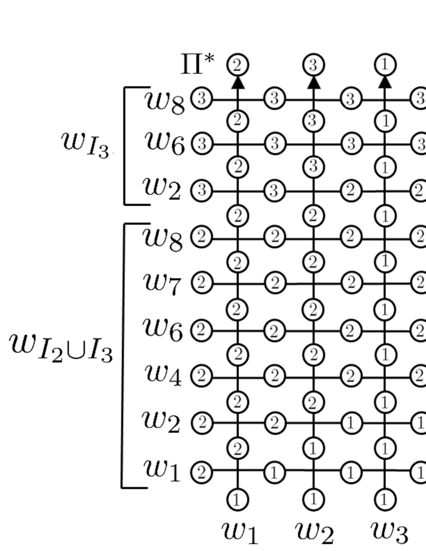
Proof.

We show by induction on $k$ . Figure 6.5 is a graphical description of the $k$ -th column of the partition function corresponding to $\tilde{X}_{II}$ or equivalently the leftmost column of the partition function $Z_{k}$ when $k\in I_{l}$ . By inductive assumption, the left boundary condition of the column which corresponds to the left boundary condition of $Z_{k}$ is given by ${\bf K}_{k}=(1^{n(I,k,2)+\cdots+n(I,k,N)},2^{|I_{2}\cup\dots\cup I_{N}|-n(I,k,2)},3^{|I_{3}\cup\dots\cup I_{N}|-n(I,k,3)},\dots,N^{|I_{N}|-n(I,k,N)})$ . We find in the same way as in Example that the empty circles in Figure 6.5 are uniquely filled with the numbers as given in Figure 6.6. This means that from this column we have products of $R$ -matrix elements denoted as $W_{k}$ , which can be read out explicitly from Figure 6.6 as $W_{k}=W_{k}^{1}W_{k}^{2}W_{k}^{3}$ where $W_{k}^{1}$ , $W_{k}^{2}$ , $W_{k}^{3}$ are (6.70), (6.71) and (6.72). Figure 6.6 also implies $Z_{k}=W_{k}Z_{k+1}$ . The right boundary of the column in Figure 6.6 is ${\bf K}_{k+1}=(1^{n(I,k+1,2)+\cdots+n(I,k+1,N)},2^{|I_{2}\cup\dots\cup I_{N}|-n(I,k+1,2)},3^{|I_{3}\cup\dots\cup I_{N}|-n(I,k+1,3)},\\ \dots,N^{|I_{N}|-n(I,k+1,N)})$ and this becomes the left boundary of $Z_{k+1}$ . ∎

To get the expression (6.66), first note $\widetilde{X}_{II}=\prod_{k=1}^{n}W_{k}=\prod_{k=1}^{n}W_{k}^{1}W_{k}^{2}W_{k}^{3}$ . Also recall the disjoint union of $I_{1},\dots,I_{N}$ is ${[}1,n{]}$ . Then one notes from the expressions (6.70), (6.71), (6.72) that $\prod_{k=1}^{n}W_{k}^{1}$ , $\prod_{k=1}^{n}W_{k}^{2}$ and $\prod_{k=1}^{n}W_{k}^{3}$ can be expressed as

$\displaystyle\prod_{k=1}^{n}W_{k}^{1}$	$\displaystyle=\displaystyle\prod_{l=1}^{N-1}\prod_{\begin{subarray}{c}j\in I_{N-l+1}\cup\cdots\cup I_{N}\\ k\in I_{1}\cup\cdots\cup I_{N-l-1}\end{subarray}}\theta(w_{j}/w_{k}),$	(6.73)
$\displaystyle\prod_{k=1}^{n}W_{k}^{2}$	$\displaystyle=\displaystyle\prod_{l=1}^{N-1}\Bigg{\{}\prod_{\begin{subarray}{c}j\in I_{N-l+1}\cup\cdots\cup I_{N}\\ k\in I_{N-l}\\ j>k\end{subarray}}\theta(w_{j}/w_{k})\prod_{\begin{subarray}{c}j\in I_{N-l+1}\cup\cdots\cup I_{N}\\ k\in I_{N-l}\\ j<k\end{subarray}}\theta(q^{2}w_{j}/w_{k})\Bigg{\}},$	(6.74)
$\displaystyle\prod_{k=1}^{n}W_{k}^{3}$	$\displaystyle=\displaystyle\theta(q^{2})^{\sum_{k=2}^{N}(k-1)\|I_{k}\|}\prod_{l=1}^{N-1}\Bigg{\{}\prod_{\begin{subarray}{c}j\in I_{N-l+1}\cup\cdots\cup I_{N}\\ k\in I_{N-l+1}\cup\cdots\cup I_{N}\\ j<k\end{subarray}}\theta(q^{2}w_{j}/w_{k})\prod_{\begin{subarray}{c}j\in I_{N-l+1}\cup\cdots\cup I_{N}\\ k\in I_{N-l+1}\cup\cdots\cup I_{N}\\ j>k\end{subarray}}\theta(q^{2}w_{j}/w_{k})\Bigg{\}}.$	(6.75)

Multiplying (6.73), (6.74) and (6.75) and rearranging, one gets (6.66).

∎

As a corollary, we obtain $N({\bf w})=\widetilde{X}_{II}/X_{II}$ as follows.

Corollary 6.7.

	$\displaystyle N({\bf w})$	$\displaystyle=\theta(q^{2})^{\sum_{k=2}^{N}(k-1)\|I_{k}\|}\prod_{1\leq k<l<N}\prod_{a\in I_{k}}\prod_{\begin{subarray}{c}b\in I_{l}\\ a<b\end{subarray}}\frac{\theta(q^{2}w_{b}/w_{a})}{\theta(w_{b}/w_{a})}\prod_{l=1}^{N-1}\Bigg{\{}\prod_{\begin{subarray}{c}j\in I_{N-l+1}\cup\cdots\cup I_{N}\\ k\in I_{1}\cup\cdots\cup I_{N-l-1}\end{subarray}}\theta(w_{j}/w_{k})$
		$\displaystyle\times\prod_{\begin{subarray}{c}j\in I_{N-l+1}\cup\cdots\cup I_{N}\\ k\in I_{N-l}\cup\cdots\cup I_{N}\\ j<k\end{subarray}}\theta(q^{2}w_{j}/w_{k})\prod_{\begin{subarray}{c}j\in I_{N-l+1}\cup\cdots\cup I_{N}\\ k\in I_{N-l+1}\cup\cdots\cup I_{N}\\ j>k\end{subarray}}\theta(q^{2}w_{j}/w_{k})\prod_{\begin{subarray}{c}j\in I_{N-l+1}\cup\cdots\cup I_{N}\\ k\in I_{N-l}\\ j>k\end{subarray}}\theta(w_{j}/w_{k})\Bigg{\}}.$

Example. For the case $N=2$ , we have

\displaystyle N({\bf w})

\displaystyle=\prod_{a\in I_{1}}\prod_{b\in I_{2}}\theta(q^{2}w_{b}/w_{a})\prod_{a\in I_{2}}\prod_{b\in I_{2}}\theta(q^{2}w_{b}/w_{a}).

Acknowledgments

This work was partially supported by grant-in-Aid for Scientific Research (C) 20K03507, 21K03176, 20K03793.

Appendix A Defining Relations of $U_{q,p}(\widehat{\mbox{\fourteeneufm gl}}_{N})$ and $U_{q,p}(\widehat{\mbox{\fourteeneufm sl}}_{N})$

A.1 $U_{q,p}(\widehat{\mathfrak{gl}}_{N})$

For $g(P),g(P+h)\in{\mathbb{F}}$ ,

	$\displaystyle g({P+h})e_{j}(z)=e_{j}(z)g({P+h}),\quad g({P})e_{j}(z)=e_{j}(z)g(P-\langle Q_{\alpha_{j}},P\rangle),$		(A.1)
	$\displaystyle g({P+h})f_{j}(z)=f_{j}(z)g(P+h-\langle{\alpha_{j}},P+h\rangle),\quad g({P})f_{j}(z)=f_{j}(z)g(P),$		(A.2)
	$\displaystyle g({P})k^{+}_{l}(z)=k^{+}_{l}(z)g(P-\langle Q_{\bar{\epsilon}_{l}},P\rangle),\quad g({P+h})k^{+}_{l}(z)=k^{+}_{l}(z)g(P+h-\langle Q_{\bar{\epsilon}_{l}},P\rangle),$
			(A.3)
	$\displaystyle\rho^{+}_{+}(z_{2}/z_{1})k^{+}_{l}(z_{1})k^{+}_{l}(z_{2})=\rho^{+}_{+}(z_{1}/z_{2})k^{+}_{l}(z_{2})k^{+}_{l}(z_{1}),\qquad(1\leq l\leq N),$		(A.4)
	$\displaystyle\rho^{+}_{+}(z_{2}/z_{1})\frac{(p^{}z_{2}/z_{1};p^{})_{\infty}(pq^{2}z_{2}/z_{1};p)_{\infty}}{(p^{}q^{2}z_{2}/z_{1};p^{})_{\infty}(pz_{2}/z_{1};p)_{\infty}}k^{+}_{j}(z_{1})k^{+}_{l}(z_{2})$
	$\displaystyle\qquad={\rho}^{+}_{+}(z_{1}/z_{2})\frac{(q^{-2}z_{1}/z_{2};p^{})_{\infty}(z_{1}/z_{z};p)_{\infty}}{(z_{1}/z_{2};p^{})_{\infty}(q^{-2}z_{1}/z_{2};p)_{\infty}}k^{+}_{l}(z_{2})k^{+}_{j}(z_{1})\quad(1\leq j<l\leq N),$		(A.5)
	$\displaystyle\frac{(p^{}q^{c+2-j}z_{2}/z_{1};p^{})_{\infty}}{(p^{}q^{c-j}z_{2}/z_{1};p^{})_{\infty}}k_{j}^{+}(z_{1})e_{j}(z_{2})=q^{-1}\frac{(q^{-c+j}z_{1}/z_{2};p^{})_{\infty}}{(q^{-c-2+j}z_{1}/z_{2};p^{})_{\infty}}e_{j}(z_{2})k_{j}^{+}(z_{1}),$		(A.6)
	$\displaystyle\frac{(p^{}q^{c-2-j}z_{2}/z_{1};p^{})_{\infty}}{(p^{}q^{c-j}z_{2}/z_{1};p^{})_{\infty}}k_{j+1}^{+}(z_{1})e_{j}(z_{2})=q\frac{(q^{-c+j}z_{1}/z_{2};p^{})_{\infty}}{(q^{-c+2+j}z_{1}/z_{2};p^{})_{\infty}}e_{j}(z_{2})k_{j+1}^{+}(z_{1}),$		(A.7)
	$\displaystyle k_{l}^{+}(z_{1})e_{j}(z_{2})k_{l}^{+}(z_{1})^{-1}=e_{j}(z_{2})\qquad\qquad(l\not=j,j+1),$		(A.8)
	$\displaystyle\frac{(pq^{-j}z_{2}/z_{1};p)_{\infty}}{(pq^{2-j}z_{2}/z_{1};p)_{\infty}}k_{j}^{+}(z_{1})f_{j}(z_{2})=q\frac{(q^{-2+j}z_{1}/z_{2};p)_{\infty}}{(q^{j}z_{1}/z_{2};p)_{\infty}}f_{j}(z_{2})k_{j}^{+}(z_{1}),$		(A.9)
	$\displaystyle\frac{(pq^{-j}z_{2}/z_{1};p)_{\infty}}{(pq^{-2-j}z_{2}/z_{1};p)_{\infty}}k_{j+1}^{+}(z_{1})f_{j}(z_{2})=q^{-1}\frac{(q^{2+j}z_{1}/z_{2};p)_{\infty}}{(q^{j}z_{1}/z_{2};p)_{\infty}}f_{j}(z_{2})k_{j+1}^{+}(z_{1}),$		(A.10)
	$\displaystyle k_{l}^{+}(z_{1})f_{j}(z_{2})k_{l}^{+}(z_{1})^{-1}=f_{j}(z_{2})\qquad\qquad(l\not=j,j+1),$		(A.11)
	$\displaystyle z_{1}\frac{(q^{2}z_{2}/z_{1};p^{})_{\infty}}{(p^{}q^{-2}z_{2}/z_{1};p^{})_{\infty}}e_{j}(z_{1})e_{j}(z_{2})=-z_{2}\frac{(q^{2}z_{1}/z_{2};p^{})_{\infty}}{(p^{}q^{-2}z_{1}/z_{2};p^{})_{\infty}}e_{j}(z_{2})e_{j}(z_{1}),$		(A.12)
	$\displaystyle z_{1}\frac{(q^{-1}z_{2}/z_{1};p^{})_{\infty}}{(p^{}qz_{2}/z_{1};p^{})_{\infty}}e_{j}(z_{1})e_{j+1}(z_{2})=-z_{2}\frac{(q^{-1}z_{1}/z_{2};p^{})_{\infty}}{(p^{}qz_{1}/z_{2};p^{})_{\infty}}e_{j+1}(z_{2})e_{j}(z_{1}),$		(A.13)
	$\displaystyle e_{j}(z_{1})e_{l}(z_{2})=e_{l}(z_{2})e_{j}(z_{1})\qquad\qquad(\|j-l\|>1)$		(A.14)
	$\displaystyle z_{1}\frac{(q^{-2}z_{2}/z_{1};p)_{\infty}}{(pq^{2}z_{2}/z_{1};p)_{\infty}}f_{j}(z_{1})f_{j}(z_{2})=-z_{2}\frac{(q^{-2}z_{1}/z_{2};p)_{\infty}}{(pq^{2}z_{1}/z_{2};p)_{\infty}}f_{j}(z_{2})f_{j}(z_{1}),$		(A.15)
	$\displaystyle z_{1}\frac{(qz_{2}/z_{1};p)_{\infty}}{(pq^{-1}z_{2}/z_{1};p)_{\infty}}f_{j}(z_{1})f_{j+1}(z_{2})=-z_{2}\frac{(qz_{1}/z_{2};p)_{\infty}}{(pq^{-1}z_{1}/z_{2};p)_{\infty}}f_{j+1}(z_{2})f_{j}(z_{1}),$		(A.16)
	$\displaystyle f_{j}(z_{1})f_{l}(z_{2})=f_{l}(z_{2})f_{j}(z_{1})\qquad\qquad(\|j-l\|>1)$		(A.17)
	$\displaystyle[e_{i}(z_{1}),f_{j}(z_{2})]=\frac{\delta_{i,j}\kappa}{q-q^{-1}}\left(\delta(q^{-c}z_{1}/z_{2})k_{j}^{-}(q^{-\frac{c}{2}}z_{1})k_{j+1}^{-}(q^{-\frac{c}{2}}z_{1})^{-1}\right.$
	$\displaystyle\left.\qquad\qquad\qquad\qquad\qquad\qquad\qquad-\delta(q^{c}z_{1}/z_{2})k_{j}^{+}(q^{-\frac{c}{2}}z_{2})k_{j+1}^{+}(q^{-\frac{c}{2}}z_{2})^{-1}\right),$		(A.18)

	$\displaystyle\frac{(p^{}q^{2}{z_{2}}/{z_{1}};p^{})_{\infty}}{(p^{}q^{-2}{z_{2}}/{z_{1}};p^{})_{\infty}}\left\{\frac{(p^{}q^{-1}{z_{1}}/{w};p^{})_{\infty}}{(p^{}qz_{1}/{w};p^{})_{\infty}}\frac{(p^{}q^{-1}{z_{2}}/w;p^{})_{\infty}}{(p^{}q{z_{2}}/w;p^{})_{\infty}}e_{j}(w)e_{i}(z_{1})e_{i}(z_{2})\right.$
	$\displaystyle\left.\qquad\qquad\qquad-[2]_{q}\frac{(p^{}q^{-1}w/{z_{1}};p^{})_{\infty}}{(p^{}qw/z_{1};p^{})_{\infty}}\frac{(p^{}q^{-1}{z_{2}}/w;p^{})_{\infty}}{(p^{}q{z_{2}}/w;p^{})_{\infty}}e_{i}(z_{1})e_{j}(w)e_{i}(z_{2})\right.$
	$\displaystyle\left.\qquad+\frac{(p^{}q^{-1}w/{z_{1}};p^{})_{\infty}}{(p^{}qw/z_{1};p^{})_{\infty}}\frac{(p^{}q^{-1}w/{z_{2}};p^{})_{\infty}}{(p^{}qw/{z_{2}};p^{})_{\infty}}e_{i}(z_{1})e_{i}(z_{2})e_{j}(w)\right\}+(z_{1}\leftrightarrow z_{2})=0,$		(A.19)
	$\displaystyle\frac{(pq^{-2}{z_{2}}/{z_{1}};p)_{\infty}}{(pq^{2}{z_{2}}/{z_{1}};p)_{\infty}}\left\{\frac{(pq{z_{1}}/{w};p)_{\infty}}{(pq^{-1}z_{1}/{w};p)_{\infty}}\frac{(pq{z_{2}}/w;p)_{\infty}}{(pq^{-1}{z_{2}}/w;p)_{\infty}}f_{j}(w)f_{i}(z_{1})f_{i}(z_{2})\right.$
	$\displaystyle\left.\qquad\qquad\qquad-[2]_{q}\frac{(pqw/{z_{1}};p)_{\infty}}{(pq^{-1}w/z_{1};p)_{\infty}}\frac{(pq{z_{2}}/w;p)_{\infty}}{(pq^{-1}{z_{2}}/w;p)_{\infty}}f_{i}(z_{1})f_{j}(w)f_{i}(z_{2})\right.$
	$\displaystyle\left.\qquad+\frac{(pqw/{z_{1}};p)_{\infty}}{(pq^{-1}w/z_{1};p)_{\infty}}\frac{(pqw/{z_{2}};p)_{\infty}}{(pq^{-1}w/{z_{2}};p)_{\infty}}f_{i}(z_{1})f_{i}(z_{2})f_{j}(w)\right\}+(z_{1}\leftrightarrow z_{2})=0\quad\|i-j\|=1,$
			(A.20)

where $\delta(z)=\sum_{n\in{\mathbb{Z}}}z^{n}$ , $\rho(z)=\rho^{+*}(z)/\rho^{+}(z)$ ,

\displaystyle\rho^{+}_{+}(z)=\frac{\{q^{2}z\}^{*}\{q^{-2}q^{2N}z\}^{*}\{z\}\{q^{2N}z\}}{\{z\}^{*}\{q^{2N}z\}^{*}\{q^{2}z\}\{q^{-2}q^{2N}z\}},\quad\{z\}=(z;q^{2N},p)_{\infty},\quad\{z\}^{*}=(z;q^{2N},p^{*})_{\infty},

and $\kappa$ is given by

\displaystyle\kappa=\frac{(p;p)_{\infty}(p^{*}q^{2};p^{*})_{\infty}}{(p^{*};p^{*})_{\infty}(pq^{2};p)_{\infty}}.

(A.21)

We treat these relations as formal Laurent series in $z,w$ and $z_{j}$ ’s. All the coefficients in $z_{j}$ ’s are well defined in the $p$ -adic topology.

A.2 $U_{q,p}(\widehat{\mathfrak{sl}}_{N})$

The defining relations of $U_{q,p}(\widehat{\mathfrak{sl}}_{N})$ consists of (2.46), (A.1), (A.2), the Serre relations (A.19) and (A.20), and the following relations.

	$\displaystyle z_{1}\frac{(q^{a_{ij}}z_{2}/z_{1};p^{})_{\infty}}{(p^{}q^{-a_{ij}}z_{2}/z_{1};p^{})_{\infty}}e_{i}(z_{1})e_{j}(z_{2})=-z_{2}\frac{(q^{a_{ij}}z_{1}/z_{2};p^{})_{\infty}}{(p^{}q^{-a_{ij}}z_{1}/z_{2};p^{})_{\infty}}e_{j}(z_{2})e_{i}(z_{1}),$		(A.22)
	$\displaystyle z_{1}\frac{(q^{-a_{ij}}z_{2}/z_{1};p)_{\infty}}{(pq^{a_{ij}}z_{2}/z_{1};p)_{\infty}}f_{i}(z_{1})f_{j}(z_{2})=-z_{2}\frac{(q^{-a_{ij}}z_{1}/z_{2};p)_{\infty}}{(pq^{a_{ij}}z_{1}/z_{2};p)_{\infty}}f_{j}(z_{2})f_{i}(z_{1}),$		(A.23)
	$\displaystyle[e_{i}(z_{1}),f_{j}(z_{2})]=\frac{\delta_{i,j}}{q-q^{-1}}\left(\delta(q^{-c}z_{1}/z_{2})\psi_{j}^{-}(q^{\frac{c}{2}}z_{2})-\delta(q^{c}z_{1}/z_{2})\psi_{j}^{+}(q^{-\frac{c}{2}}z_{2})\right).$		(A.24)

References

[1] M. Aganagic and A. Okounkov, Elliptic Stable Envelopes, Journal of the American Mathematical Society 34, (2021), 79-133.
[2] J.Beck, Braid Group Action and Quantum Affine Algebras. Comm.Math.Phys.165 (1994), 555-568.
[3] V.Chari and A.N.Pressley, Yangians and $R$ -matrices, L’Enseignement Math. 36 (1990), 267–302.
[4] V. Chari and A. N. Pressley, Quantum affine algebras, Comm. Math. Phys. 142 (1991), 261–283.
[5] V. Chari and A. N. Pressley, Quantum affine algebras and their representations, Proceedings of the Canadian Mathematical Society Annual Seminar Representations of Groups, Banff, 1994
[6] V. Chari and A. N. Pressley, A Guide to Quantum Groups, Cambridge University Press, Cambridge, 1994.
[7] V.G. Drinfeld, Hopf Algebras and the Quantum Yang-Baxter Equation, Soviet Math.Dokl. 32 (1985) 264–268; V.G. Drinfeld, Quantum Groups, Proceedings of the ICM, Berkeley (1986).
[8] V.G. Drinfeld, A New Realization of Yangians and Quantized Affine Algebras. Soviet Math. Dokl. 36 (1988) 212-216.
[9] P.Etingof and A.Varchenko, Solutions of the Quantum Dynamical Yang-Baxter Equation and Dynamical Quantum Groups, Comm.Math.Phys. 196 (1998), 591–640 ; Exchange Dynamical Quantum Groups, Comm.Math.Phys. 205 (1999), 19–52.
[10] R.M.Farghly, H.Konno, K.Oshima, Elliptic Algebra $U_{q,p}(\widehat{\mathfrak{g}})$ and Quantum Z-algebras, Alg. Rep. Theory 18 (2014), 103-135.
[11] G. Felder, Elliptic Quantum Groups, Proc. ICMP Paris-1994 (1995), 211–218.
[12] I. M. Gelfand and M. L. Tsetlin, Finite-Dimensional Representations of the Group of Uni-modular Matrices, Dokl. Akad. Nauk SSSR 71 (1950), 825-828 (Russian).
[13] V.Gorbounov, R.Rimányi, V.Tarasov and A.Varchenko, Cohomology of the Cotangent Bundle of a Flag Variety as a Yangian Bethe Algebra, J.Geom.Phys., 74 (2013) 56–86.
[14] M.Jimbo, A $q$ -difference analogue of $U(\mathfrak{g})$ and the Yang-Baxter Equation, Lett.Math.Phys. 10 (1985) 63–69.
[15] M. Jimbo, in Field Theory, Quantum Gravity and Strings, Lecture Notes in Physics 246, Springer, 1985, p. 335.
[16] M.Jimbo, A $q$ -Analogue of $U({\mathfrak{gl}}(N+1))$ , Hecke Algebra, and the Yang-Baxter Equation, Lett.Math.Phys. 11 (1986) 247–252.
[17] M. Jimbo, H. Konno, S. Odake and J. Shiraishi, Quasi-Hopf Twistors for Elliptic Quantum Groups, Transformation Groups 4 (1999) 303–327.
[18] M. Jimbo, H. Konno, S. Odake and J. Shiraishi, Elliptic Algebra $U_{q,p}(\widehat{\mathfrak{sl}}_{2})$ : Drinfeld Currents and Vertex Operators, Comm. Math. Phys. 199 (1999), 605–647
[19] E.Koelink and H.Rosengren, Harmonic Analysis on the $SU(2)$ Dynamical Quantum Group, Acta.Appl.Math., 69 (2001), 163–220.
[20] T. Kojima and H. Konno, The Elliptic Algebra $U_{q,p}(\widehat{\mathfrak{sl}}_{N})$ and the Drinfeld Realization of the Elliptic Quantum Group $\mathcal{B}_{q,\lambda}(\widehat{\mathfrak{sl}}_{N})$ , Comm. Math. Phys. 239 (2003), 405–447.
[21] H. Konno, Elliptic Quantum Group $U_{q,p}(\widehat{\mathfrak{sl}}_{2})$ , Hopf Algebroid Structure and Elliptic Hypergeometric Series, Journal of Geometry and Physics 59 (2009), 1485-1511.
[22] H. Konno, Elliptic Weight Functions and Ellitpic $q$ -KZ equation, J. Int. Sys. 2 (2017), 1-43.
[23] H. Konno, Elliptic Quantum Groups $U_{q,p}(\widehat{{\mathfrak{gl}}}_{N})$ and $E_{q,p}(\widehat{{\mathfrak{gl}}}_{N})$ , Advanced Studies in Pure Mathematics 76 (2018), 347-417.
[24] H. Konno, Elliptic Stable Envelops and Finite-Dimensional Representations of Elliptic Quantum Group, J. Int. Sys. 3 (2018), 1-43.
[25] Y.Koyama, Staggered Polarization of Vertex Models with $U_{q}(\widehat{\mathfrak{sl}(n)})$ - Symmetry, Comm.Math.Phys. 164 (1994), 277–291.
[26] D.Maulik and A.Okounkov, Quantum Groups and Quantum Cohomology, Astérisque 408 (2019), Societe mathematique de France
[27] A. Molev, Yangians and classical Lie algebras, Mathematical Surveys and Monographs, vol. 143, American Mathematical Society, Providence, RI,. 2007.
[28] M. Nazarov and V. Tarasov, Yangians and Gelfand-Zetlin Bases, Publ.RIMS, Kyoto Univ. 30 (1994), 459–478.
[29] M. Nazarov and V. Tarasov, Representations of Yangians with Gelfand-Zetlin Bases, Journal fur die Reine und Angewandte Mathematik 496 (1998), 181-212.
[30] A.Okounkov, Lectures on K-theoretic Computations in Enumerative Geometry. (2015), arXiv: 1512.07363.
[31] R. Rimányi, V. Tarasov, A. Varchenko, Trigonometric Weight Functions as $K$ -theoretic Stable Envelope Maps for the Cotangent Bundle of a Flag Variety, J. Geom. Phys. 94 (2015), 81-119.
[32] R.Rimányi, V.Tarasov and A.Varchenko, Elliptic and $K$ -theoretic Stable Envelopes and Newton Polytopes, Selecta Math. (N.S.) 25 (2019), no. 1, Paper No.16, 43 pp.
[33] V.Tarasov, Irreducible Monodromy Matrices for the $R$ Matrix of the $XXZ$ Model and Local Lattice Quantum Hamiltonians, Theor.Math.Phys. 63 (1985) 440–454.
[34] H. Rosengren, An Izergin-Korepin-type identity for the 8VSOS model, with applications to alternating sign matrices, Adv. in Appl. Math. 43 (2009) 137–155.
[35] K.Ueno, T.Takebayashi and Y.Shibukawa, Gelfand-Zetlin Basis for $U_{q}({\mathfrak{gl}}(N+1))$ Modules, Lett.Math.Phys. 18 (1989) 215–221.

Gelfand-Tsetlin Bases for Elliptic Quantum Groups

Abstract

1 Introduction

2 Elliptic Quantum Groups Uq,p​(𝔤​𝔩^N)U_{q,p}(\widehat{{\mathfrak{gl}}}_{N}) and Eq,p​(𝔤​𝔩^N)E_{q,p}(\widehat{\mathfrak{gl}}_{N})

2.1 Preliminaries

2.2 The elliptic dynamical RR-matrix of the 𝔤​𝔩^N\widehat{{\mathfrak{gl}}}_{N} type

2.3 The elliptic algebra Uq,p​(𝔤​𝔩^N)U_{q,p}(\widehat{{\mathfrak{gl}}}_{N})

Definition 2.1.

Theorem 2.2.

Corollary 2.3.

2.4 The elliptic algebra Uq,p​(𝔰​𝔩^N)U_{q,p}(\widehat{\mathfrak{sl}}_{N})

Definition 2.4.

2.5 The elliptic algebra Eq,p​(𝔤​𝔩^N)E_{q,p}(\widehat{{\mathfrak{gl}}}_{N})

Definition 2.5.

2.6 Isomorphism between Uq,p​(𝔤​𝔩^N)U_{q,p}(\widehat{\mathfrak{gl}}_{N}) and Eq,p​(𝔤​𝔩^N)E_{q,p}(\widehat{\mathfrak{gl}}_{N})

Proposition 2.6.

Definition 2.7.

Lemma 2.8 ([23], Lemma 6.10).

Definition 2.9.

Theorem 2.10.

2.7 Quantum determinant

Definition 2.1.

Proposition 2.2.

Proposition 2.3.

Definition 2.11.

Proposition 2.12.

Corollary 2.13.

Proposition 2.14.

Proof.

Proposition 2.15.

2.8 Coalgebra structure

Proposition 2.16.

3 Finite-Dimensional Representations

3.1 Level-0 highest weight representation

Proposition 3.1.

Proof.

Definition 3.2.

Proposition 3.3.

Definition 3.4.

Definition 3.5.

Proposition 3.6.

Definition 3.7.

Theorem 3.8.

Theorem 3.9.

Definition 3.10 ([34]).

Definition 3.11.

Theorem 3.12.

Corollary 3.13.

Proposition 3.14.

Proof.

Corollary 3.15.

Definition 3.16.

Corollary 3.17.

3.2 Proof of the if part of Theorem 3.12

Proposition 3.18.

Proof.

Proof.

4 Representations of Uq,p​(𝔤​𝔩^2)U_{q,p}(\widehat{\mathfrak{gl}}_{2})

Theorem 4.1.

Definition 4.2.

Proposition 4.3.

Theorem 4.4.

4.1 The Gelfand-Tsetlin bases

Theorem 4.5.

Lemma 4.6.

5 The Gelfand-Tsetlin Bases for Uq,p​(𝔤​𝔩^N)U_{q,p}(\widehat{\mathfrak{gl}}_{N})-modules

Proposition 5.1.

Proof.

Theorem 5.2.

Proof.

6 Tensor Product of the Vector Representations

Definition 6.1.

Lemma 6.1.

Proof.

6.1 The vector representation

Proposition 6.2.

6.2 The Gelfand-Tsetlin bases for V^w1​⊗~​⋯​⊗~​V^wn\widehat{V}_{w_{1}}\widetilde{\otimes}\cdots\widetilde{\otimes}\widehat{V}_{w_{n}}

Definition 6.2.

Proposition 6.3.

Proof.

2 Elliptic Quantum Groups $U_{q,p}(\widehat{{\mathfrak{gl}}}_{N})$ and $E_{q,p}(\widehat{\mathfrak{gl}}_{N})$

2.2 The elliptic dynamical $R$ -matrix of the $\widehat{{\mathfrak{gl}}}_{N}$ type

2.3 The elliptic algebra $U_{q,p}(\widehat{{\mathfrak{gl}}}_{N})$

2.4 The elliptic algebra $U_{q,p}(\widehat{\mathfrak{sl}}_{N})$

2.5 The elliptic algebra $E_{q,p}(\widehat{{\mathfrak{gl}}}_{N})$

2.6 Isomorphism between $U_{q,p}(\widehat{\mathfrak{gl}}_{N})$ and $E_{q,p}(\widehat{\mathfrak{gl}}_{N})$

4 Representations of $U_{q,p}(\widehat{\mathfrak{gl}}_{2})$

5 The Gelfand-Tsetlin Bases for $U_{q,p}(\widehat{\mathfrak{gl}}_{N})$ -modules

6.2 The Gelfand-Tsetlin bases for $\widehat{V}_{w_{1}}\widetilde{\otimes}\cdots\widetilde{\otimes}\widehat{V}_{w_{n}}$

6.3 Relation between $\xi_{\boldsymbol{\nu}}$ and $\widetilde{\xi}_{I}$

Appendix A Defining Relations of $U_{q,p}(\widehat{\mbox{\fourteeneufm gl}}_{N})$ and $U_{q,p}(\widehat{\mbox{\fourteeneufm sl}}_{N})$

A.1 $U_{q,p}(\widehat{\mathfrak{gl}}_{N})$

A.2 $U_{q,p}(\widehat{\mathfrak{sl}}_{N})$