GDP: Stabilized Neural Network Pruning via Gates with Differentiable Polarization
Abstract
Model compression techniques are recently gaining explosive attention for obtaining efficient AI models for various real time applications. Channel pruning is one important compression strategy, and widely used in slimming various DNNs. Previous gate-based or importance-based pruning methods aim to remove channels whose “importance” are smallest. However, it remains unclear what criteria the channel importance should be measured on, leading to various channel selection heuristics. Some other sampling-based pruning methods deploy sampling strategy to train sub-nets, which often causes the training instability and the compressed model’s degraded performance. In view of the research gaps, we present a new module named Gates with Differentiable Polarization (GDP), inspired by principled optimization ideas. GDP can be plugged before convolutional layers without bells and whistles, to control the on-and-off of each channel or whole layer block. During the training process, the polarization effect will drive a subset of gates to smoothly decrease to exact zero, while other gates gradually stay away from zero by a large margin. When training terminates, those zero-gated channels can be painlessly removed, while other non-zero gates can be absorbed into the succeeding convolution kernel, causing completely no interruption to training nor damage to the trained model. Experiments conducted over CIFAR-10 and ImageNet datasets show that the proposed GDP algorithm achieves the state-of-the-art performance on various benchmark DNNs at a broad range of pruning ratios. We also apply GDP to DeepLabV3Plus-ResNet50 on the challenging Pascal VOC segmentation task, whose test performance sees no drop (even slightly improved) with over 60% FLOPs saving.
1 Introduction
Model compression techniques recently attract many attentions from both industry and academic research communities for compressing Deep Neural Networks (DNNs) to satisfy devices with limited computing and storage capabilities. One common model compression method is pruning, which includes unstructured pruning (i.e., weights sparsification) [4, 20, 38, 46, 66] and structured pruning (e.g., channel pruning and kernel pruning) [78]. Unstructured pruning removes individual weight, which results in sparse connection and requires sparse matrix operations supports. The structured pruning eliminates an entire neuron or a block at once, leaving the model’s structure and connections intact and thus having no special requirements for hardware or specific libraries. In this paper, we focus on the latter.
Importance-based pruning methods usually prune channels/blocks whose importance are small, but it remains unclear what criteria the importance should be measured on, leading to various importance selection heuristics, such as the magnitude of weights [74], first-order or second-order information of weights [11, 56, 59], knockoff features of filters [69] and so on. One recent track of works follow the sparse learning optimization routines, utilizing LASSO or group LASSO [24, 48, 74] to regularize training weights. However, these methods need to prune from a skewed yet continuous histogram of weights values, and the selection of the pruning threshold [20] is critical yet ad-hoc, taking Figure 1(a) for example. Moreover, removing many small yet non-zero weights will inevitably damage the network, and often need to fine-tune before the next pruning schedule, causing iterative pruning-finetuning loop [19, 42, 48, 55].


Besides the importance-based pruning methods, some sampling-based methods [14, 34, 53, 87, 22, 84] either sample a sub-network or calculate expectations over whole network to train, utilizing Gambul-Softmax [31], STE [1] or Bernoulli distribution [66, 84] strategies. These methods may potentially cause either unstable training due to equiprobable sampling (i.e. sample a completely different sub-net when the probability is nearly uniformly distributed at the beginning of training), or converging at local minimum due to deterministic sampling (i.e. sample nearly the same sub-net when the probability becomes deterministic), thus need various ad-hoc manual designs [14].
| FLOPs ratio | Before removing | After removing | After fine-tuning |
| 43.8% | 69.962 | 69.962 | 70.150 |
To bridge these research gaps, we introduce a novel scheme called Gates with Differentiable Polarization (GDP), which can easily plug-and-play with any existing convolutional or fully connected layer. It does not rely on any specific module such as Batch Normalization (BN) [29] or ReLU [15], and contains fewer hyper-parameters to tune during optimization than those minimax optimization methods [41, 77] used in resource-constrained model compression. The core idea of GDP is to encourage gate values to update smoothly towards polarization (some are exact zero, others stay away from zero by a large margin) during training, so that the exact-zero-gated channels/blocks can be painlessly removed and other gates be absorbed into conv/fully-connected kernels, without causing any damage, as illustrated in Figure 1(b) and Table 1.
Our main highlights are summarized as follows:
-
•
Core Idea of Polarization: GDP is designed to push a large interval between exact zero gates and non-zero gates while preserving the gradient-friendly optimization. This is particularly favored, and enables us to directly remove zero-gated channels/blocks and absorb other gates to the conv/fully-connected kernels with no performance impact when training terminates.
-
•
Stability, Consistency and Light-Weight: GDP gets rid of ad-hoc thresholding nor any probabilistic sampling/expectation. That makes it (1) easy to use, with nearly no manual crafting; (2) produce stable and smooth training; (3) incur almost no computational or time overhead; and (4) not rely on any specific modules such as BN or ReLU.
-
•
State-of-the-Art Results: Experiments on CIFAR-10 and ImageNet classification tasks show that GDP outperforms all previous competitors with clear margins. GDP can obtain slightly improved performance in the Pascal VOC segmentation task with DeepLabV3Plus-ResNet50, while reducing more than 60% FLOPs.
2 Related Work
Model compression techniques are broadly applied in many research fields successfully, such as GAN [70, 13], Recommendation system [65] and so on. There are many model compression techniques proposed to solve different problems, including network pruning [28, 48, 88], weights quantization [30, 32, 35], knowledge distillation [25, 27], architecture searching [47, 90], weights hashing [12] and so on. Some works [19, 61, 71, 76, 16] have tried to unify aforementioned techniques into one framework, which can slim network comprehensively. In this paper, we only focus on pruning strategy to achieve SOTA compression results by leveraging a differentiable polarized gate design and we want to emphasize that our GDP method can be adjusted into a unified compression framework easily.
2.1 Pruning Strategies
Importance based pruning:
One straightforward way to prune a network is to throw out less important components. [24, 42, 43, 48, 74] use group LASSO to regularize convolution kernels or other scale factors during training, leaving some weights values small. However, these works suffer from how to choose pruning threshold. Furthermore, [80] points out that channels or blocks with smaller weights norm may not necessarily means that they are less important. Besides weights norm metric, some other works [7, 39, 56, 58, 38, 52] explore some new importance metrics, such as first-order, second-order taylor expansions of weights and so on. The designing of importance metrics is still an open problem to explore.
Sampling based pruning:
Sampling process is not differentiable, however [22, 34] use Gumbel-Softmax [31] trick to make sampling process differentiable during network training, thus can be used in pruning network. While [14] uses straight-through estimator [1] on a step function controlled by probability oscillating around 0.5. [51, 84] relaxes the intractable L0 regularization by using hard-sigmoid function as gate function instead, then sample a sub-net by Gumbel-Softmax similarly as previous work or by Bernoulli [84]. These methods sample sub-networks stochastically, while we continually adapt a single network. DARTS [47] introduced differentiable architecture search by formulating the output of a layer as the expectation of all input candidate edges and then choosing edges with the largest probabilities, which can be treated as a general pruning method. We do not want to compute expectation, since it cannot accurately depict real sub-net during training.
Other variants:
Beyond above two categories, several works choose to prune networks gradually by reinforcement learning [23, 68]; meta-learning [49]; evolutionary methods [18] and so on. Furthermore, [83] trains a proxy network to represent the accuracy of sub-nets with different channel configurations, and then greedily slim a network. [3] considers a generalized pruning on all dimensional of network to progressively train once for all sub-nets. All these methods may suffer from the computational resources overhead and their complicated designs may hinder the popularization and application of them. However, our pruning method is straightforward and takes about the same amount of time as training of baseline model.
A series of recent works [41, 62, 77, 85] formulate the network pruning problem into a constrained minimax optimization problem, and then use ADMM method [2] to solve it. However, these methods inevitably introduce many hyper-parameters (like dual variables) to tune. Instead, our method is simple yet efficient, with fewer parameters to tune during compression.
3 Methods
We introduce the details of our pruning algorithm in this section, including a special gate design, the FLOPs reformulation based on it and the proposed alternative proximal optimization method.
3.1 Pruning via Gates
For CNNs compression, instead of directly measuring the channel importance as in previous work, we plug trainable gates immediately before regular convolution (‘regular’ is used to distinguish from ‘depth-wise’) or fully connected layers to control the on-and-off of each channel or even whole block. Some works [34, 80, 82] utilize BN or ReLU layer as gates, however, a channel being judged as unimportant now doesn’t mean it won’t be important after a series of channel-wise operations, such as pooling, depth-wise convolution [8], et al. What’s more, some networks may not contains BN or ReLU. So, we plug gates immediately before the position where information from different channels are going to merge. Different from [14], we do not plug gates before depth-wise convolution, which does not merge information from different channels. Figure 2 illustrates the positions where the gates should be plugged into, without losing generalization, simply taking a residual block in MobileNet-V2 as example.
Specifically, let be the input of the -th layer convolution kernel , where , and represent the number of channels, height and width of the input feature map respectively; and is the number of output channels and kernel size of the convolution kernel, respectively. We can insert a gate vector with dimension as channel-wise scaling factors for , before it is convolved by . That is, the output, , of the convolution operation is
| (1) |
where is the channel-wise multiplication, and is the convolution operation. One can easily control the on-and-off of these channels by manipulating . In GDP, some gates smoothly decrease to be exact zeros, while others stay away from zeros by a large margin gradually. Then we can safely remove channels corresponding to the zero-gates, and absorb the others to the successive convolution kernel. By this way, the sub-net can be got with performance same to the super-net.

3.2 Differentiable Polarized Gates
Previous gate-based methods usually use some optimization tricks to make the gate differentiable, such as Gumbel-Softmax trick used in sampling-based method and L1-norm penalty in regularization based method and so on. These methods either cause unstable training process or cannot obtain exact zero values. To ensure the stability and effectiveness of model pruning, the desired gate should have following properties: 1. be differentiable for back-propagation with simpler tricks than complicated sampling mechanism; 2. the values are better to range in ; 3. the distribution of values should be two modes, one mode keeps exact zeros while others stay away from zeros obviously. Also, we do not want to construct an expectation-based or sampling-based resource calculation, which can not represent the accurate resource of a specific sub-net. [66] constructs a heuristic bi-modal regularizer to satisfy above conditions, while we choose the smoothed L0 formulation from principled optimization methods [75]:
| (2) |
where is a small positive number. This function has the following important property:
| (3) |


We can observe that when is small enough, approaches to zero only at the points where get exact zeros or ones, otherwise infinity. It means that the function can only stay stable at 0 or 1. Different from Gumbel-Softmax with decreasing temperature, Function (12) can be exactly zero even when is not small. This good quality implies to us that we can regard as gate, plugging into the neural network we want to compress. The subscript will be omitted in the following text when not causing misunderstanding. Theoretically, here can either be an newly introduced trainable parameters, or can directly be the norm of convolution kernel weights. We will analyze both settings in ablation study. We choose the former setting in our algorithm, since it works better than latter one.
During training, gradually decays by a factor smaller than one, and all the gates vary smoothly between 0 and 1. When the training terminates, becomes small enough, and some gates become exact zeros while the others approach ones. Then, we can prune network explicitly by removing the channels corresponding to zero-gates and absorbing other close-to-ones gates into convolution kernel . In almost all of our experiments, the performance of the pruned-net is exactly same as that of the super-net before explicitly pruning. In section 4, we will show that the explicitly pruned sub-nets without fine-tuning, already keep pace with or even better than previous state-of-the-art works. We think that the performance consistency between pruned-net and super-net is a good property to help us choose good candidate sub-nets.
3.3 Resource-constrained Pruning Formulation
Some works [14, 87] calculate the resource by expectation, which do not represent the accurate resource of a specific sub-net. Instead, we formulate the resource by a bilinear function with respect to the number of channels of each layer [77]. Specifically, if the resource is FLOPs, a bilinear function can strictly model it for most common CNNs. In this paper, we directly take FLOPs as resource to illustrate our pruning algorithm. The FLOPs of a CNN can be accurately formulated as:
| (5) |
Where is the number of channels in the -th layer, is the coefficients of bilinear function. Specifically, for the -th layer with channels, gates with introduced learnable parameters are inserted immediately before the -th convolution layer. Then, according to Function (3), the resource function (5) can be rewritten as:
| (6) |
where is -norm of a vector. The final objective function can be formulated as below:
| (7) |
where is the original training loss function, denotes all the learnable weights of original network, denotes all the introduced learnable parameters for gates, is the total number of layers, and is a balance factor.
3.4 Optimization via Alternative Relaxation
Objective function (7) is not easy to solve due to the existence of -norm. and in can be updated by common gradient descent algorithm, just as did in normal training of baseline model. For , we can use proximal-SGD [57] to update . The proximal operator is defined as:
| (8) |
Formulation (8) is a proximal problem with a bi-linear -norm format. We solve it iteratively by alternative relaxation. Specifically, we alternately update by relaxing to while treating other as constants at current time, and then exchange the variables and constants roles to perform relaxing operation again. The details are shown in Algorithm 1. Note that in line 1, we do not relax to when it is treated as constant.
Line 1 in Algorithm 1 is proximal -norm problem, which has closed form solution:
| (9) |
where , and the subscript means the -th entry of the vector.
In fact, general proximal -norm problem also has closed form solution.
The reason we choose to relax -norm to -norm in our algorithm is that all entries of in proximal -norm operation can shrink a small step at each iteration, which may compete with the change caused by .
This effect exists regardless of the initialization value of .
However, for proximal -norm operation, the entries with large initialization values will always fluctuate in a small range, while the other entries initialized with small values quickly vanish at the first few iterations and very hard to recover later by .
We find in our experiments that proximal -norm operation works robustly while proximal -norm operation is very sensitive to initialization of .
As for convergence of Algorithm 1, with large number of simulations, we find that it always converges quickly, although it’s not necessarily the globally optimal solution. An simple illustration example is shown in Figure 3.4, which converge quickly with very few iterations. In all experiments in this paper, we find iteration works well enough.
![[Uncaptioned image]](https://cdn.awesomepapers.org/papers/55d68eb7-0e87-4d43-9945-7f8bcd304911/iterL0L1_v2.png)
: A simple example to show the convergence of Algorithm 1. The objective function here is set to be , where , and . init1 denotes the initialization with and , while init2 denotes the initialization with and .
4 Experiments
We conduct classification experiments on CIFAR-10 [36] dataset with ResNet-56, VGG-16 and MobileNet-V2, and ImageNet ILSVRC-12 dataset [9] with MobileNet-V1/V2, ResNet-50 respectively. Our main experiments are done by introducing learnable parameters while we also do ablation study with using convolution kernel as parameters for gate function in Equation (12). We compare GDP with previous works: EagleE [40], PFS [72], MetaP [49], AMC [23], NetAdapt [79], DCP [89], GFS [81], LeGR [7], DMCP [18], SCP [34], SLRTD [60], OICSR [42], Taylor [56], CCP [59], GD [82], Hinge [43], CURL [54], HRank [44], LFPC [22], C-SGD [10], SCOP [69], AutoSlim [83], ABCpruner [45], DMC [14], VCNNP [86]. It should be pointed out that AutoSlim [83] uses totally different training settings from most works, and prunes from more heavier models, thus not comparable. Also we should mention that MDP [17] is more likely NAS method for searching sub-nets; EagleE [40] uses adaptive BN strategy to improve various sub-nets evaluation. We did not compare with these special papers on CIFAR-10, due to their extremely good performance reported, with a large gap to other papers. Although aforementioned two papers are not fair to compare with our pruning method, our simple yet effective method still achieves better performance than these out-of-scope papers on ImageNet with various benchmark networks. The drawing scripts containing all numerical values of all figures are left in supplementary materials.
4.1 Implementation Details
and settings
For all experiments, the and are initialized with 1.0 and 0.1 respectively. The learning rate of is one tenth of that of the other network parameters for classification task and there is no weight decay on when training. For CIFAR-10, we train 350 epochs with decaying by 0.96 every epoch, while for ImageNet, we train 140 epochs with decaying by 0.9 every epoch. For DeepLabV3Plus-ResNet50, we train it for 60k iterations, and decay by 0.97 every 120 iterations. Also, the initial learning rate of is 9e-4 as it is different for classifier and backbone. We smooth the shrinkage of when necessary.
CIFAR-10 Experiments
We randomly flipped horizontally, randomly cropped size of 32 with padding 4 on images, and perform normalization to augment the data when training. Table 2 shows the performance of CIFAR-10 on various network structure. The network structure for VGG-16 and ResNet-56 is same as [44]. MobileNet-V2 is from LeGR [7], but we do not find the CIFAR-10 results in LeGR. Note that the structure of MobileNet-V2 for CIFAR-10 may differ in different works. We train it with cosine learning rate [50] without label smoothing [67]. These experiments are conducted on single NVIDIA 2080Ti GPU.
| Method | Baseline(%) | Ratio(%) | Abs. Acc. | Acc. | |
| VGG-16 | PFS | 93.44 | 50 | 93.63 | 0.19 |
| SCP | 93.85 | 33.77 | 93.79 | -0.06 | |
| VCNNP | 93.25 | 39.1 | 93.18 | -0.07 | |
| Hinge | 94.02 | 60.93 | 93.59 | -0.43 | |
| HRank | 93.96 | 46.4 | 93.43 | -0.53 | |
| GDP (Ours) | 93.89 | 30.55 | 93.99 | 0.1 | |
| ResNet-56 | PFS | 93.23 | 50 | 93.05 | -0.18 |
| ABCPruner | 93.26 | 45.87 | 93.23 | -0.03 | |
| HRank | 93.26 | 50 | 93.17 | -0.09 | |
| SCOP | 93.7 | 44 | 93.64 | -0.06 | |
| LFPC | 93.59 | 52.9 | 93.72 | 0.13 | |
| LeGR | 93.9 | 47 | 93.7 | -0.2 | |
| GDP (Ours) | 93.9 | 34.36 | 93.55 | -0.35 | |
| GDP (Ours) | 93.9 | 46.65 | 93.97 | 0.07 | |
| Mobile-V2 | SCOP | 94.48 | 59.7 | 94.24 | -0.24 |
| MDP | 95.02 | 71.29 | 95.14 | 0.12 | |
| DMC | 94.23 | 60 | 94.49 | 0.26 | |
| GDP (Ours) | 94.89 | 53.78 | 95.15 | 0.26 |
ImageNet Experiments
We conduct experiments on ImageNet ILSVRC-12 dataset [37] with MobileNet-V1/V2 [26, 64] and ResNet-50 [21]. We use this dataset the same way as PyTorch official example111https://github.com/pytorch/examples/blob/master/imagenet/main.py.
For MobileNet-V1, the initial learning rate is set to 0.1 and decayed by 0.1 every 35 epochs for training. No label smoothing is used, same to most previous works. Figure 5 shows the performance of GDP compared to other works.
MobileNet-V2 is designed with inverted residual blocks, and it is more efficient than MobileNet-V1, which is more challenging for model pruning. Same as most previous works, we use label smoothing and cosine learning rate to boost performance. Figure 6 shows the performance of GDP compared with other works. We can clearly see that GDP has enjoyed great advantages over previous works. We do not show AutoSlim [83] here because it prune MobileNet-V2 from a more heavier super-net (MobileNet-V2 1.5) and used many training tricks. We do not use this settings to keep comparable with most others works.
ResNet-50 is a network with much more FLOPs. Some works use cosine learning rate and/or label smoothing while others not, the baseline also varies dramatically. So we plot two version curves, one with cosine learning rate and label smoothing, the other neither. See Figure 7, GDP is also superior than other works. Experiments for MobileNet-V1/V2 are conducted on two NVIDIA 2080Ti GPUs, while experiments for ResNet-50 are on two NVIDIA V100 GPUs.


Pascal VOC with DeepLabv3+
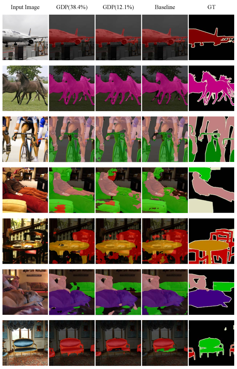
DeepLabv3+ [6] is designed with a decoder module besides the Atrous Spatial Pyramid Pooling(ASPP) to extend DeepLabv3 [5] and get better segmentation results. It contains a more complex network structure than classification tasks, so we choose it to demonstrate the generalization and robustness of GDP. We use ResNet-50 as backbone, and follow the same training settings as public implementation 222https://github.com/VainF/DeepLabV3Plus-Pytorch. The output stride (OS) for training and validation is 16. Table 3 shows the mIoU of Pascal VOC segmentation task, and several visual results are shown in supplementary materials. For the sub-net with 38.4% FLOPs, we are surprised to find that the branch with atrous-rate 18 in the ASPP module is totally pruned, the branch with atrous-rate 12 only 6 channels left, however, gaining slightly better performance.
Furthermore, we also deploy GDP method in Style Transfer task, based on official PyTorch implementation of [33], achieving great performance on pruned models with large portion of FLOPs savings. Visual results of pruned models are shown in supplementary materials.
| FLOPs(%) | 38.4 | 23.3 | 12.1 | 5.2 | Baseline |
| mIOU | 0.779 | 0.767 | 0.721 | 0.666 | 0.774 |
4.2 Discussion
Polarization
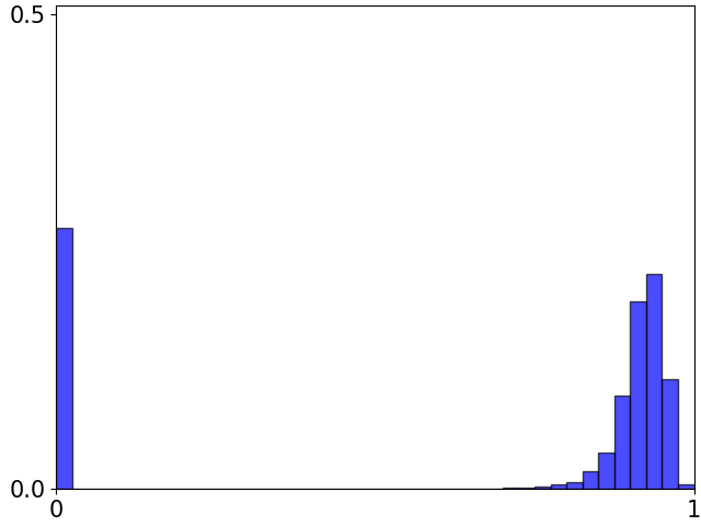
Figure 9 shows density distributions of gate values during the training process. We can see that the density distributions of gates change smoothly and the number of zero-gates becomes stable after epoch 70. The polarization depends on the value of . A larger results in a smoother gate with less polarization; a smaller makes (12) closer to norm but with less numerical stability. An ablation study for the effects of is attached in supplementary materials. Our method is robust to different values of .
Consistency
We do not need to sample sub-net or calculate expectation when training. Figure 11 shows the training stability of GDP. When training terminates, there is only one candidate sub-net left. Different value of in Function (7) result in sub-net with different FLOPs and performance. We want the performance of the super-net to reflect the performance of the final sub-net as much as possible. We set multiple hyper-parameters to run the GDP compression training. Figure 4.2 reflects the relationship between performance of super-net before explicitly pruning and the sub-net after fine-tuning.
![[Uncaptioned image]](https://cdn.awesomepapers.org/papers/55d68eb7-0e87-4d43-9945-7f8bcd304911/gw_v3.png)


![[Uncaptioned image]](https://cdn.awesomepapers.org/papers/55d68eb7-0e87-4d43-9945-7f8bcd304911/consistency_v2.png)
: The relationship between Top-1 accuracy of super-net before explicitly pruning and that of the corresponding sub-net after fine-tuning. The correlation coefficient is 0.993. We can see that the accuracy of super-net effectively reflects that of the final sub-net. This experiments are conducted on ImageNet with MobileNet-V1.


4.3 Ablation studies
Not introducing
There is an alternative solution that instead of introducing the learnable parameters , we can also use the existing convolution kernels weights as in Equation (12). The objective function is then becomes:
| (10) |
For the -th layer convolution kernel , we can let where , is the indication of input channels, and substitute defined here for in Equation (6). In this case, we initialize in every gate to one-tenth of the corresponding , so the initial value of all gates is , the same to when is introduced. The performance is plotted in Figure 4.2, labeled with “Gates of Conv Kernels”. We guess that the relatively poor performance of using may be caused by dual roles of both feature extraction and gate controlling, which has the opposite thoughts from [63, 73], or caused by the occasional instability of the norm of when is small enough.
as regularization
was originally used as regularization term added to the original objective function of smooth L0 optimization [75]. Follow this idea, we can also naively define our objective function as bellow:
| (11) |
The reason we did not take this approach is similar to above. The norm of is occasionally unstable when training, maybe caused by . However, if we introduce as in Equation (7), it is not itself but to participate in the network forward. is stably taking values in range . The performance is shown in Figure 4.2, labeled with “Naive SL0”.
Pruning from Scratch
Figure 4.2 also shows some results by pruning from scratch (labeled with “GDP Scratch”) rather than from a well-trained model. With the same hyper-parameters, the pruning speed of “GDP Scratch” became particularly faster and a more compressed sub-net was obtained. This relatively poor performance might result from that some important channels have no resistance to being pruned before they get learned well enough.
5 Numerical Result
We put the numerical result in Table 4 and Table 5 for better comparison with future work, although it is already attached in supplementary materials.
| FLOPs(%) | 26.7 | 35.8 | 45.1 | 50.4 | 58.3 | 71.4 |
| MV1(top1) | 68.5 | 69.9 | 70.7 | 71.3 | 71.9 | 72.4 |
| FLOPs(%) | 18.9 | 25.4 | 30.4 | 34.4 | 38.7 | 49.0 |
| Res50(top1) | 74.1 | 75.1 | 75.6 | 76.1 | 76.4 | 77.1 |
| FLOPs(%) | 13.0 | 16.5 | 22.0 | 26.4 | 30.4 | 36.1 | 43.8 | 52.1 | 62.4 | 77.6 | 96.1 |
| MV2(top1) | 60.3 | 62.6 | 65.4 | 66.8 | 67.8 | 68.9 | 70.2 | 70.9 | 71.8 | 72.5 | 73.1 |
6 Ablation study for
The smooth L0 function is defined as:
| (12) |
The polarization depends on the value of . A larger results in a smoother gate with less polarization; a smaller makes gate function closer to norm but with less numerical stability. Fig. 12 shows different decaying rates of with their corresponding compression ratios and Top-1 accuracy. We can see that GDP is robust to the final value of ranging from to , which is a really big range.

Besides the decaying rate, we also study the effect of initial value of , as shown in Fig. 13. We can also see the robustness of GDP with respect to different initial values.

7 Visual results for style transfer and semantic segmentation
For style transfer, it can be seen that our pruned model can achieve similar results without hurting perceptual quality, as shown in Fig. 14 and Fig. 15. Also, our pruned model can even achieve better boundary quality compared with and semantic segmentation baseline, as shown in Fig. 16


8 Conclusion
In this paper, we proposed a novel differentiable polarized gate module in network pruning task and obtain state-of-the-arts performance on various benchmark experiments. Comparing with other optimization-based pruning methods, the advantages of our method are five folds: simpler to implementation; fewer hyper-parameters to tune; obtain good sub-nets easily; take less time; not rely on any specific network structure. The disadvantage is that the model pruning ratio cannot be specified in advance, which now need to manually adjust the value of to balance the accuracy and resource consumption of network. We leave this problem in future works. The gates with differentiable polarization proposed in this paper can also be easily extended into neural architecture search (NAS) tasks.
References
- [1] Yoshua Bengio, Nicholas Léonard, and Aaron Courville. Estimating or propagating gradients through stochastic neurons for conditional computation. arXiv preprint arXiv:1308.3432, 2013.
- [2] Stephen Boyd, Neal Parikh, and Eric Chu. Distributed optimization and statistical learning via the alternating direction method of multipliers. Now Publishers Inc, 2011.
- [3] Han Cai, Chuang Gan, Tianzhe Wang, Zhekai Zhang, and Song Han. Once-for-all: Train one network and specialize it for efficient deployment. In International Conference on Learning Representations, 2020.
- [4] Shih-Kang Chao, Zhanyu Wang, Yue Xing, and Guang Cheng. Directional pruning of deep neural networks. Advances in Neural Information Processing Systems, 33, 2020.
- [5] Liang Chieh Chen, George Papandreou, Florian Schroff, and Hartwig Adam. Rethinking atrous convolution for semantic image segmentation. 2017.
- [6] Liang-Chieh Chen, Yukun Zhu, George Papandreou, Florian Schroff, and Hartwig Adam. Encoder-decoder with atrous separable convolution for semantic image segmentation. In Proceedings of the European conference on computer vision (ECCV), pages 801–818, 2018.
- [7] Ting-Wu Chin, Ruizhou Ding, Cha Zhang, and Diana Marculescu. Towards efficient model compression via learned global ranking. In Proceedings of the IEEE/CVF Conference on Computer Vision and Pattern Recognition, pages 1518–1528, 2020.
- [8] François Chollet. Xception: Deep learning with depthwise separable convolutions. In Proceedings of the IEEE conference on computer vision and pattern recognition, pages 1251–1258, 2017.
- [9] Jia Deng, Wei Dong, Richard Socher, Li-Jia Li, Kai Li, and Li Fei-Fei. Imagenet: A large-scale hierarchical image database. In 2009 IEEE conference on computer vision and pattern recognition, pages 248–255. Ieee, 2009.
- [10] Xiaohan Ding, Guiguang Ding, Yuchen Guo, and Jungong Han. Centripetal sgd for pruning very deep convolutional networks with complicated structure. In Proceedings of the IEEE/CVF Conference on Computer Vision and Pattern Recognition, pages 4943–4953, 2019.
- [11] Xiaohan Ding, Guiguang Ding, Xiangxin Zhou, Yuchen Guo, Jungong Han, and Ji Liu. Global sparse momentum sgd for pruning very deep neural networks. arXiv preprint arXiv:1909.12778, 2019.
- [12] Elad Eban, Yair Movshovitz-Attias, Hao Wu, Mark Sandler, Andrew Poon, Yerlan Idelbayev, and Miguel A Carreira-Perpinán. Structured multi-hashing for model compression. In Proceedings of the IEEE/CVF Conference on Computer Vision and Pattern Recognition, pages 11903–11912, 2020.
- [13] Yonggan Fu, Wuyang Chen, Haotao Wang, Haoran Li, Yingyan Lin, and Zhangyang Wang. Autogan-distiller: Searching to compress generative adversarial networks. ICML, 2020.
- [14] Shangqian Gao, Feihu Huang, Jian Pei, and Heng Huang. Discrete model compression with resource constraint. In IEEE Conference on Computer Vision and Pattern Recognition (CVPR 2020), 2020.
- [15] Xavier Glorot, Antoine Bordes, and Yoshua Bengio. Deep sparse rectifier neural networks. In Proceedings of the fourteenth international conference on artificial intelligence and statistics, pages 315–323. JMLR Workshop and Conference Proceedings, 2011.
- [16] Shupeng Gui, Haotao Wang, Chen Yu, Haichuan Yang, Zhangyang Wang, and Ji Liu. Model compression with adversarial robustness: A unified optimization framework. Neural Information Processing Systems, 2019.
- [17] Jinyang Guo, Wanli Ouyang, and Dong Xu. Multi-dimensional pruning: A unified framework for model compression. In Proceedings of the IEEE/CVF Conference on Computer Vision and Pattern Recognition, pages 1508–1517, 2020.
- [18] Shaopeng Guo, Yujie Wang, Quanquan Li, and Junjie Yan. Dmcp: Differentiable markov channel pruning for neural networks. In Proceedings of the IEEE/CVF Conference on Computer Vision and Pattern Recognition, pages 1539–1547, 2020.
- [19] Song Han, Huizi Mao, and William J Dally. Deep compression: Compressing deep neural networks with pruning, trained quantization and huffman coding. arXiv preprint arXiv:1510.00149, 2015.
- [20] Song Han, Jeff Pool, John Tran, and William J Dally. Learning both weights and connections for efficient neural networks. arXiv preprint arXiv:1506.02626, 2015.
- [21] Kaiming He, Xiangyu Zhang, Shaoqing Ren, and Jian Sun. Deep residual learning for image recognition. In Proceedings of the IEEE conference on computer vision and pattern recognition, pages 770–778, 2016.
- [22] Yang He, Yuhang Ding, Ping Liu, Linchao Zhu, Hanwang Zhang, and Yi Yang. Learning filter pruning criteria for deep convolutional neural networks acceleration. In Proceedings of the IEEE/CVF Conference on Computer Vision and Pattern Recognition, pages 2009–2018, 2020.
- [23] Yihui He, Ji Lin, Zhijian Liu, Hanrui Wang, Li-Jia Li, and Song Han. Amc: Automl for model compression and acceleration on mobile devices. In Proceedings of the European Conference on Computer Vision (ECCV), pages 784–800, 2018.
- [24] Yihui He, Xiangyu Zhang, and Jian Sun. Channel pruning for accelerating very deep neural networks. In Proceedings of the IEEE International Conference on Computer Vision, pages 1389–1397, 2017.
- [25] G. Hinton, O. Vinyals, and J. Dean. Distilling the knowledge in a neural network. Computer Science, 14(7):38–39, 2015.
- [26] Andrew G Howard, Menglong Zhu, Bo Chen, Dmitry Kalenichenko, Weijun Wang, Tobias Weyand, Marco Andreetto, and Hartwig Adam. Mobilenets: Efficient convolutional neural networks for mobile vision applications. arXiv preprint arXiv:1704.04861, 2017.
- [27] Zehao Huang and Naiyan Wang. Like what you like: Knowledge distill via neuron selectivity transfer. arXiv preprint arXiv:1707.01219, 2017.
- [28] Forrest N Iandola, Song Han, Matthew W Moskewicz, Khalid Ashraf, William J Dally, and Kurt Keutzer. Squeezenet: Alexnet-level accuracy with 50x fewer parameters and¡ 0.5 mb model size. arXiv preprint arXiv:1602.07360, 2016.
- [29] Sergey Ioffe and Christian Szegedy. Batch normalization: Accelerating deep network training by reducing internal covariate shift. In International conference on machine learning, pages 448–456. PMLR, 2015.
- [30] Benoit Jacob, Skirmantas Kligys, Bo Chen, Menglong Zhu, Matthew Tang, Andrew Howard, Hartwig Adam, and Dmitry Kalenichenko. Quantization and training of neural networks for efficient integer-arithmetic-only inference. In Proceedings of the IEEE Conference on Computer Vision and Pattern Recognition, pages 2704–2713, 2018.
- [31] Eric Jang, Shixiang Gu, and Ben Poole. Categorical reparameterization with gumbel-softmax. International Conference on Learning Representations (ICLR), 2017.
- [32] Qing Jin, Linjie Yang, and Zhenyu Liao. Adabits: Neural network quantization with adaptive bit-widths. In Proceedings of the IEEE/CVF Conference on Computer Vision and Pattern Recognition, pages 2146–2156, 2020.
- [33] Justin Johnson, Alexandre Alahi, and Li Fei-Fei. Perceptual losses for real-time style transfer and super-resolution. In European conference on computer vision, pages 694–711. Springer, 2016.
- [34] Minsoo Kang and Bohyung Han. Operation-aware soft channel pruning using differentiable masks. In International Conference on Machine Learning, pages 5122–5131. PMLR, 2020.
- [35] Raghuraman Krishnamoorthi. Quantizing deep convolutional networks for efficient inference: A whitepaper. arXiv preprint arXiv:1806.08342, 2018.
- [36] Alex Krizhevsky, Geoffrey Hinton, et al. Learning multiple layers of features from tiny images. 2009.
- [37] Alex Krizhevsky, Ilya Sutskever, and Geoffrey E Hinton. Imagenet classification with deep convolutional neural networks. Advances in neural information processing systems, 25:1097–1105, 2012.
- [38] Jaeho Lee, Sejun Park, Sangwoo Mo, Sungsoo Ahn, and Jinwoo Shin. Layer-adaptive sparsity for the magnitude-based pruning. In International Conference on Learning Representations, 2021.
- [39] Namhoon Lee, Thalaiyasingam Ajanthan, and Philip HS Torr. Snip: Single-shot network pruning based on connection sensitivity. arXiv preprint arXiv:1810.02340, 2018.
- [40] Bailin Li, Bowen Wu, Jiang Su, and Guangrun Wang. Eagleeye: Fast sub-net evaluation for efficient neural network pruning. In European Conference on Computer Vision, pages 639–654. Springer, 2020.
- [41] Hongjia Li, Ning Liu, Xiaolong Ma, Sheng Lin, Shaokai Ye, Tianyun Zhang, Xue Lin, Wenyao Xu, and Yanzhi Wang. Admm-based weight pruning for real-time deep learning acceleration on mobile devices. In Proceedings of the 2019 on Great Lakes Symposium on VLSI, pages 501–506, 2019.
- [42] Jiashi Li, Qi Qi, Jingyu Wang, Ce Ge, Yujian Li, Zhangzhang Yue, and Haifeng Sun. Oicsr: Out-in-channel sparsity regularization for compact deep neural networks. In Proceedings of the IEEE/CVF Conference on Computer Vision and Pattern Recognition, pages 7046–7055, 2019.
- [43] Yawei Li, Shuhang Gu, Christoph Mayer, Luc Van Gool, and Radu Timofte. Group sparsity: The hinge between filter pruning and decomposition for network compression. In Proceedings of the IEEE/CVF Conference on Computer Vision and Pattern Recognition, pages 8018–8027, 2020.
- [44] Mingbao Lin, Rongrong Ji, Yan Wang, Yichen Zhang, Baochang Zhang, Yonghong Tian, and Ling Shao. Hrank: Filter pruning using high-rank feature map. In Proceedings of the IEEE/CVF Conference on Computer Vision and Pattern Recognition, pages 1529–1538, 2020.
- [45] Mingbao Lin, Rongrong Ji, Yuxin Zhang, Baochang Zhang, Yongjian Wu, and Yonghong Tian. Channel pruning via automatic structure search. arXiv preprint arXiv:2001.08565, 2020.
- [46] Tao Lin, Sebastian U Stich, Luis Barba, Daniil Dmitriev, and Martin Jaggi. Dynamic model pruning with feedback. arXiv preprint arXiv:2006.07253, 2020.
- [47] Hanxiao Liu, Karen Simonyan, and Yiming Yang. DARTS: Differentiable architecture search. In International Conference on Learning Representations, 2019.
- [48] Zhuang Liu, Jianguo Li, Zhiqiang Shen, Gao Huang, Shoumeng Yan, and Changshui Zhang. Learning efficient convolutional networks through network slimming. In Proceedings of the IEEE International Conference on Computer Vision, pages 2736–2744, 2017.
- [49] Zechun Liu, Haoyuan Mu, Xiangyu Zhang, Zichao Guo, Xin Yang, Kwang-Ting Cheng, and Jian Sun. Metapruning: Meta learning for automatic neural network channel pruning. In Proceedings of the IEEE/CVF International Conference on Computer Vision, pages 3296–3305, 2019.
- [50] Ilya Loshchilov and Frank Hutter. Sgdr: Stochastic gradient descent with warm restarts. arXiv preprint arXiv:1608.03983, 2016.
- [51] Christos Louizos, Max Welling, and Diederik P. Kingma. Learning sparse neural networks through l0 regularization. In International Conference on Learning Representations, 2018.
- [52] Ekdeep Singh Lubana and Robert Dick. A gradient flow framework for analyzing network pruning. In International Conference on Learning Representations, 2021.
- [53] Jian-Hao Luo and Jianxin Wu. Autopruner: An end-to-end trainable filter pruning method for efficient deep model inference. Pattern Recognition, 107:107461, 2020.
- [54] Jian-Hao Luo and Jianxin Wu. Neural network pruning with residual-connections and limited-data. In Proceedings of the IEEE/CVF Conference on Computer Vision and Pattern Recognition, pages 1458–1467, 2020.
- [55] Jian-Hao Luo, Jianxin Wu, and Weiyao Lin. Thinet: A filter level pruning method for deep neural network compression. In Proceedings of the IEEE international conference on computer vision, pages 5058–5066, 2017.
- [56] Pavlo Molchanov, Arun Mallya, Stephen Tyree, Iuri Frosio, and Jan Kautz. Importance estimation for neural network pruning. In Proceedings of the IEEE/CVF Conference on Computer Vision and Pattern Recognition, pages 11264–11272, 2019.
- [57] Atsushi Nitanda. Stochastic proximal gradient descent with acceleration techniques. Advances in Neural Information Processing Systems, 27:1574–1582, 2014.
- [58] Sejun Park, Jaeho Lee, Sangwoo Mo, and Jinwoo Shin. Lookahead: a far-sighted alternative of magnitude-based pruning. arXiv preprint arXiv:2002.04809, 2020.
- [59] Hanyu Peng, Jiaxiang Wu, Shifeng Chen, and Junzhou Huang. Collaborative channel pruning for deep networks. In International Conference on Machine Learning, pages 5113–5122. PMLR, 2019.
- [60] Anh-Huy Phan, Konstantin Sobolev, Konstantin Sozykin, Dmitry Ermilov, Julia Gusak, Petr Tichavskỳ, Valeriy Glukhov, Ivan Oseledets, and Andrzej Cichocki. Stable low-rank tensor decomposition for compression of convolutional neural network. In European Conference on Computer Vision, pages 522–539. Springer, 2020.
- [61] Antonio Polino, Razvan Pascanu, and Dan Alistarh. Model compression via distillation and quantization. arXiv preprint arXiv:1802.05668, 2018.
- [62] Ao Ren, Tianyun Zhang, Shaokai Ye, Jiayu Li, Wenyao Xu, Xuehai Qian, Xue Lin, and Yanzhi Wang. Admm-nn: An algorithm-hardware co-design framework of dnns using alternating direction methods of multipliers. In Proceedings of the Twenty-Fourth International Conference on Architectural Support for Programming Languages and Operating Systems, pages 925–938, 2019.
- [63] Tim Salimans and Diederik P Kingma. Weight normalization: A simple reparameterization to accelerate training of deep neural networks. arXiv preprint arXiv:1602.07868, 2016.
- [64] Mark Sandler, Andrew Howard, Menglong Zhu, Andrey Zhmoginov, and Liang-Chieh Chen. Mobilenetv2: Inverted residuals and linear bottlenecks. In Proceedings of the IEEE conference on computer vision and pattern recognition, pages 4510–4520, 2018.
- [65] Jiayi Shen, Haotao Wang, Shupeng Gui, Jianchao Tan, Zhangyang Wang, and Ji Liu. {UMEC}: Unified model and embedding compression for efficient recommendation systems. In International Conference on Learning Representations, 2021.
- [66] Suraj Srinivas, Akshayvarun Subramanya, and R Venkatesh Babu. Training sparse neural networks. In Proceedings of the IEEE conference on computer vision and pattern recognition workshops, pages 138–145, 2017.
- [67] Christian Szegedy, Vincent Vanhoucke, Sergey Ioffe, Jon Shlens, and Zbigniew Wojna. Rethinking the inception architecture for computer vision. In Proceedings of the IEEE conference on computer vision and pattern recognition, pages 2818–2826, 2016.
- [68] Mingxing Tan, Bo Chen, Ruoming Pang, Vijay Vasudevan, Mark Sandler, Andrew Howard, and Quoc V Le. Mnasnet: Platform-aware neural architecture search for mobile. In Proceedings of the IEEE/CVF Conference on Computer Vision and Pattern Recognition, pages 2820–2828, 2019.
- [69] Yehui Tang, Yunhe Wang, Yixing Xu, Dacheng Tao, Chunjing Xu, Chao Xu, and Chang Xu. Scop: Scientific control for reliable neural network pruning. arXiv preprint arXiv:2010.10732, 2020.
- [70] Haotao Wang, Shupeng Gui, Haichuan Yang, Ji Liu, and Zhangyang Wang. Gan slimming: All-in-one gan compression by a unified optimization framework. In European Conference on Computer Vision, pages 54–73. Springer, 2020.
- [71] Tianzhe Wang, Kuan Wang, Han Cai, Ji Lin, Zhijian Liu, Hanrui Wang, Yujun Lin, and Song Han. Apq: Joint search for network architecture, pruning and quantization policy. In Proceedings of the IEEE/CVF Conference on Computer Vision and Pattern Recognition, pages 2078–2087, 2020.
- [72] Yulong Wang, Xiaolu Zhang, Lingxi Xie, Jun Zhou, Hang Su, Bo Zhang, and Xiaolin Hu. Pruning from scratch. In Proceedings of the AAAI Conference on Artificial Intelligence, volume 34, pages 12273–12280, 2020.
- [73] Ziyu Wang, Tom Schaul, Matteo Hessel, Hado Hasselt, Marc Lanctot, and Nando Freitas. Dueling network architectures for deep reinforcement learning. In International conference on machine learning, pages 1995–2003. PMLR, 2016.
- [74] Wei Wen, Chunpeng Wu, Yandan Wang, Yiran Chen, and Hai Li. Learning structured sparsity in deep neural networks. arXiv preprint arXiv:1608.03665, 2016.
- [75] Jianhong Xiang, Huihui Yue, Xiangjun Yin, and Linyu Wang. A new smoothed l0 regularization approach for sparse signal recovery. Mathematical Problems in Engineering, 2019, 2019.
- [76] Haichuan Yang, Shupeng Gui, Yuhao Zhu, and Ji Liu. Automatic neural network compression by sparsity-quantization joint learning: A constrained optimization-based approach. In Proceedings of the IEEE/CVF Conference on Computer Vision and Pattern Recognition, pages 2178–2188, 2020.
- [77] Haichuan Yang, Yuhao Zhu, and Ji Liu. Ecc: Platform-independent energy-constrained deep neural network compression via a bilinear regression model. In Proceedings of the IEEE/CVF Conference on Computer Vision and Pattern Recognition, pages 11206–11215, 2019.
- [78] Tien-Ju Yang, Andrew Howard, Bo Chen, Xiao Zhang, Alec Go, Mark Sandler, Vivienne Sze, and Hartwig Adam. Netadapt: Platform-aware neural network adaptation for mobile applications. In Proceedings of the European Conference on Computer Vision (ECCV), September 2018.
- [79] Tien-Ju Yang, Andrew Howard, Bo Chen, Xiao Zhang, Alec Go, Mark Sandler, Vivienne Sze, and Hartwig Adam. Netadapt: Platform-aware neural network adaptation for mobile applications. In Proceedings of the European Conference on Computer Vision (ECCV), pages 285–300, 2018.
- [80] Jianbo Ye, Xin Lu, Zhe Lin, and James Z Wang. Rethinking the smaller-norm-less-informative assumption in channel pruning of convolution layers. arXiv preprint arXiv:1802.00124, 2018.
- [81] Mao Ye, Chengyue Gong, Lizhen Nie, Denny Zhou, Adam Klivans, and Qiang Liu. Good subnetworks provably exist: Pruning via greedy forward selection. In International Conference on Machine Learning, pages 10820–10830. PMLR, 2020.
- [82] Zhonghui You, Kun Yan, Jinmian Ye, Meng Ma, and Ping Wang. Gate decorator: Global filter pruning method for accelerating deep convolutional neural networks. arXiv preprint arXiv:1909.08174, 2019.
- [83] Jiahui Yu and Thomas Huang. Autoslim: Towards one-shot architecture search for channel numbers. arXiv preprint arXiv:1903.11728, 2019.
- [84] Xin Yuan, Pedro Savarese, and Michael Maire. Growing efficient deep networks by structured continuous sparsification. arXiv preprint arXiv:2007.15353, 2020.
- [85] Tianyun Zhang, Shaokai Ye, Kaiqi Zhang, Jian Tang, Wujie Wen, Makan Fardad, and Yanzhi Wang. A systematic dnn weight pruning framework using alternating direction method of multipliers. In Proceedings of the European Conference on Computer Vision (ECCV), pages 184–199, 2018.
- [86] Chenglong Zhao, Bingbing Ni, Jian Zhang, Qiwei Zhao, Wenjun Zhang, and Qi Tian. Variational convolutional neural network pruning. In Proceedings of the IEEE/CVF Conference on Computer Vision and Pattern Recognition, pages 2780–2789, 2019.
- [87] Yu Zhao and Chung-Kuei Lee. Differentiable channel pruning search. arXiv preprint arXiv:2010.14714, 2020.
- [88] Michael Zhu and Suyog Gupta. To prune, or not to prune: exploring the efficacy of pruning for model compression. arXiv preprint arXiv:1710.01878, 2017.
- [89] Zhuangwei Zhuang, Mingkui Tan, Bohan Zhuang, Jing Liu, Yong Guo, Qingyao Wu, Junzhou Huang, and Jinhui Zhu. Discrimination-aware channel pruning for deep neural networks. arXiv preprint arXiv:1810.11809, 2018.
- [90] Barret Zoph and Quoc V Le. Neural architecture search with reinforcement learning. arXiv preprint arXiv:1611.01578, 2016.