Gaussian unitary ensemble with jump discontinuities and the coupled Painlevé II and IV systems

Xiao-Bo Wu¹¹1School of Mathematics and Computer Science, Shangrao Normal University, Shangrao 334001, China. E-mail: [email protected] and Shuai-Xia Xu²²2Institut Franco-Chinois de l’Energie Nucléaire, Sun Yat-sen University, Guangzhou 510275, China. E-mail: [email protected]

Abstract We study the orthogonal polynomials and the Hankel determinants associated with Gaussian weight with two jump discontinuities. When the degree $n$ is finite, the orthogonal polynomials and the Hankel determinants are shown to be connected to the coupled Painlevé IV system. In the double scaling limit as the jump discontinuities tend to the edge of the spectrum and the degree $n$ grows to infinity, we establish the asymptotic expansions for the Hankel determinants and the orthogonal polynomials, which are expressed in terms of solutions of the coupled Painlevé II system. As applications, we re-derive the recently found Tracy-Widom type expressions for the gap probability of there being no eigenvalues in a finite interval near the the extreme eigenvalue of large Gaussian unitary ensemble and the limiting conditional distribution of the largest eigenvalue in Gaussian unitary ensemble by considering a thinned process.

2010 Mathematics Subject Classification: 33E17; 34M55; 41A60

Keywords and phrases: Random matrices; Gaussian unitary ensemble; Tracy-Widom distribution; Painlevé equations; Hankel determinants; orthogonal polynomials; Riemann-Hilbert approach.

1 Introduction and statement of results

Consider the Gaussian Unitary Ensemble (GUE), where the joint probability density function of the eigenvalues is given by

\rho_{n}(\lambda_{1},...,\lambda_{n})=\frac{1}{Z_{n}}\prod_{i=1}^{n}e^{-\lambda_{i}^{2}}\prod_{1\leq i<j\leq n}^{n}|\lambda_{i}-\lambda_{j}|^{2};

(1.1)

see [15, 23]. Here $Z_{n}$ , known as the partition function, is a normalization constant. It is well known that the density function (1.1) can be expressed in the determinantal form

\rho_{n}(\lambda_{1},...,\lambda_{n})=\det[K_{n}(\lambda_{i},\lambda_{j})]_{1\leq i,j\leq n},

(1.2)

where

K_{n}(x,y)=e^{-\frac{1}{2}(x^{2}+y^{2})}\sum_{k=0}^{n-1}H_{k}(x)H_{k}(y).

(1.3)

The polynomial $H_{k}(x)$ therein is the $k$ -th degree monic orthogonal polynomial with respect to the Gaussian weight $e^{-x^{2}}$ , which is the Hermite polynomial except for a constant [24, Eq. (18.5.13)].

Introduce the Hankel determinant

	$\displaystyle D_{n}(s_{1},s_{2};\omega_{1},\omega_{2})$	$\displaystyle=\det\left(\int_{\mathtt{R}}x^{j+k}w(x;s_{1},s_{2};\omega_{1},\omega_{2})dx\right)_{j,k=0}^{n-1}$
		$\displaystyle=\frac{1}{n!}\int_{-\infty}^{\infty}\cdots\int_{-\infty}^{\infty}\prod_{i=1}^{n}w(x_{j};s_{1},s_{2};\omega_{1},\omega_{2})\prod_{1\leq i<j\leq n}^{n}(x_{i}-x_{j})^{2}dx_{1}\cdots dx_{n},$		(1.4)

where

w(x;s_{1},s_{2};\omega_{1},\omega_{2})=e^{-x^{2}}\left\{\begin{array}[]{cc}1&x<s_{1},\\ \omega_{1}&s_{1}<x<s_{2},\\ \omega_{2}&x>s_{2},\end{array}\right.

(1.5)

with the constant $\omega_{k}\geqslant 0,k=1,2$ . If $\omega_{1}=\omega_{2}=1$ , the Hankel determinant $D_{n}(s_{1},s_{2};1,1)$ is corresponding to the pure Gaussian weight $e^{-x^{2}}$ and can be evaluated explicitly

D_{n}^{\texttt{GUE}}=D_{n}(s_{1},s_{2};1,1)=(2\pi)^{n/2}2^{-n^{2}/2}\prod_{k=1}^{n-1}k!~{};

(1.6)

see [23, Equation (4.1.5)]. There is a system of monic orthogonal polynomials $\pi_{n}(x)=\pi_{n}(x;s_{1},s_{2})=x^{n}+\cdots$ , orthogonal with respect to the weight function $w(x)=w(x;s_{1},s_{2};\omega_{1},\omega_{2})$ ,

\int_{\mathbb{R}}\pi_{m}(x)\pi_{n}(x)w(x)dx=\gamma_{n}^{-2}\delta_{m,n},\quad m,n\in\mathbb{N}.

(1.7)

The orthogonal polynomials satisfy the three term recurrence relation

z\pi_{n}(z)=\pi_{n+1}(z)+\alpha_{n}\pi_{n}(z)+\beta_{n}^{2}\pi_{n-1}(z),

(1.8)

where $\alpha_{n}=\alpha_{n}(s_{1},s_{2})$ and $\beta_{n}=\beta_{n}(s_{1},s_{2})$ are the recurrence coefficients. The polynomials $\gamma_{n}\pi_{n}(x)$ are the normalized orthogonal polynomials and the leading coefficients $\gamma_{n}=\gamma_{n}(s_{1},s_{2})$ are connected to the Hankel determinant $D_{n}(s_{1},s_{2})=D_{n}(s_{1},s_{2};\omega_{1},\omega_{2})$ by

D_{n}(s_{1},s_{2})=\prod_{j=0}^{n-1}\gamma_{j}^{-2}(s_{1},s_{2}).

(1.9)

Consider the gap probability that there is no eigenvalues in the finite interval $(s_{1},s_{2})$ for the GUE matrices. On account of (1.1) and (1), the gap probability can be expressed as a ratio of the Hankel determinants

\texttt{Pro}(\lambda_{j}\not\in(s_{1},s_{2}):j=1...n)=\frac{D_{n}(s_{1},s_{2};0,1)}{D_{n}^{\texttt{GUE}}},

(1.10)

where $\lambda_{1}<,...,\lambda_{n}$ are the eigenvalues of a matrix in GUE and $D_{n}(s_{1},s_{2};\omega_{1},\omega_{2})$ is defined in (1). For the gap probability on the infinite interval $(s,+\infty)$ , we have the distribution of the largest eigenvalue

\texttt{Pro}(\lambda_{n}<s)=\frac{D_{n}(s,s;0,0)}{D_{n}^{\texttt{GUE}}}.

(1.11)

In the large $n$ limit, the distribution of the largest eigenvalue converges to the celebrated Tracy-Widom distribution

\lim_{n\to+\infty}\texttt{Pro}(\lambda_{n}<\sqrt{2n}+\frac{s}{\sqrt{2}n^{1/6}})=\exp\left(-\int_{s}^{+\infty}(x-s)q_{\texttt{HM}}^{2}(x)dx\right),

(1.12)

where $q_{\texttt{HM}}(s)$ is the Hastings-Mcleod solution of the second Painlevé equation $q^{\prime\prime}(x)-2q^{3}(x)-xq(x)=0$ with the asymptotic behavior $q_{\texttt{HM}}(x)\sim{\rm Ai}(x)$ as $x\to+\infty$ ; see [25].

We proceed to consider the thinned process in GUE by removing each eigenvalues $\lambda_{1}<,...,\lambda_{n}$ of the GUE independently with probability $p\in(0,1)$ ; see [2, 3]. It is observed in [3] that the remaining and removed eigenvalues can be interpreted as observed and unobserved particles, respectively. If we know the information that the largest observed particle $\lambda^{T}_{\max}$ is less that $y$ , then the conditional distribution of the largest eigenvalue $\lambda_{n}$ of the original GUE can be expressed by the ratio of Hankel determiants

\texttt{Pro}(\lambda_{n}<x|\lambda^{T}_{\max}<y)=\frac{D_{n}(y,x;p,0)}{D_{n}(y,x;p,p)},\quad x>y,

(1.13)

and

\texttt{Pro}(\lambda_{n}<x|\lambda^{T}_{\max}<y)=\frac{D_{n}(x,y;0,0)}{D_{n}(x,y;p,p)},\quad x<y,

(1.14)

with $D_{n}(s_{1},s_{2};\omega_{1},\omega_{2})$ defined in (1); see [5, 8] and [1, 7]. It is noted that other thinned random matrices in the situation of circular ensemble is considered in [5] and also in [4] with applications in the studies of Riemann zeros.

Recently, the limits of (1.10) and (1.13) are studied in [6, 8] by considering the Fredholm determinants of the Airy kernel with several discontinuities. More generally, the limits of the gap probabilities on any finite union of intervals near the extreme eigenvalues are considered in [8]. In [27], the second author of the present paper and Dai derive the asymptotics of (1.13) via the Fredholm determinants of the Painlevé XXXIV kernel which is a generalization of the Airy kernel. In both [8] and [27], Tracy-Widom type expressions for the limiting distributions are established by using solutions to the coupled Painlevé II system. The Hankel determinants and orthogonal polynomials associated with the Gaussian weight with one jump discontinuity have also been considered in [1, 16, 17, 22, 26, 28] with applications in random matrices.

The present work is devoted to the studies of the Hankel determinants and the orthogonal polynomials associated with the Gaussian weight with two jump discontinuities both as the degree $n$ is finite and as $n$ tends to infinity. When the degree $n$ is finite, we show that the Hankel determinants and the orthogonal polynomials are described by the coupled Painlevé IV system. As the jump discontinuities tend to the largest eigenvalue of GUE and the degree $n$ grows to infinity, we establish asymptotic expansions for the Hankel determinants and the orthogonal polynomials. The asymptotics are expressed in terms of solutions to the coupled Painlevé II system. As applications, our results reproduce the asymptotic expansions of the gap probability in a finite interval near the largest eigenvalue of GUE and the conditional distribution of largest eigenvalue of GUE as defined in (1.10) and (1.13), respectively, which are obtained previously in [8, 27].

1.1 Statement of results

The coupled Painlevé IV system

We introduce the Hamiltonian

H_{\texttt{IV}}(a_{1},a_{2},b_{1},b_{2};x;s)=-2(a_{1}b_{1}+a_{2}b_{2}+n)(a_{1}+a_{2})+2(a_{1}b_{1}(x-s)+a_{2}b_{2}(x+s)+nx)-(a_{1}b_{1}^{2}+a_{2}b_{2}^{2}),

(1.15)

which is a special Garnier system in two variables in the studies of the classification of 4-dimensional Painlevé-type equations by Kawakami, Nakamura and Sakai [21, Equations (3.12)-(3.13)]. The coupled Painlevé IV system can be written as the following Hamiltonian system

\left\{\begin{array}[]{l}\frac{da_{1}}{dx}=\frac{\partial H_{\texttt{IV}}}{\partial b_{1}}(a_{1},a_{2},b_{1},b_{2};x,s)=-2a_{1}(a_{1}+a_{2}+b_{1}-x+s),\\ \frac{da_{2}}{dx}=\frac{\partial H_{\texttt{IV}}}{\partial b_{2}}(a_{1},a_{2},b_{1},b_{2};x,s)=-2a_{2}(a_{1}+a_{2}+b_{2}-x-s),\\ \frac{db_{1}}{dx}=-\frac{\partial H_{\texttt{IV}}}{\partial a_{1}}(a_{1},a_{2},b_{1},b_{2};x,s)=b_{1}^{2}+2b_{1}(2a_{1}+a_{2}-x+s)+2(a_{2}b_{2}+n),\\ \frac{db_{2}}{dx}=-\frac{\partial H_{\texttt{IV}}}{\partial a_{2}}(a_{1},a_{2},b_{1},b_{2};x,s)=b_{2}^{2}+2b_{2}(a_{1}+2a_{2}-x-s)+2(a_{1}b_{1}+n).\end{array}\right.

(1.16)

Eliminating $b_{1}$ and $b_{2}$ from the system, we find that $a_{1}$ and $a_{2}$ solve a couple of second order nonlinear differential equations

\left\{\begin{array}[]{l}\frac{\mathtt{d}^{2}a_{1}}{\mathtt{d}x^{2}}-\frac{1}{2a_{1}}\left(\frac{\mathtt{d}a_{1}}{\mathtt{d}x}\right)^{2}-6a_{1}(a_{1}+a_{2})^{2}+8a_{1}(a_{1}+a_{2})x-8a_{1}^{2}s+2(2n-1)a_{1}-2a_{1}(x-s)^{2}=0,\\ \frac{\mathtt{d}^{2}a_{2}}{\mathtt{d}x^{2}}-\frac{1}{2a_{2}}\left(\frac{\mathtt{d}a_{2}}{\mathtt{d}x}\right)^{2}-6a_{2}(a_{1}+a_{2})^{2}+8a_{2}(a_{1}+a_{2})x+8a_{2}^{2}s+2(2n-1)a_{2}-2a_{2}(x+s)^{2}=0.\end{array}\right.

(1.17)

If $a_{2}=0$ , we recover from the above equations the classical Painlevé IV equation (see [13] and [24, Equation (32.2.4)] )

y_{\texttt{IV}}^{\prime\prime}=\frac{1}{2y_{\texttt{IV}}}y_{\texttt{IV}}^{\prime 2}+\frac{3}{2}y_{\texttt{IV}}^{3}+4xy_{\texttt{IV}}^{2}+2(x^{2}+1-2n)y_{\texttt{IV}},\quad y_{\texttt{IV}}(x)=-2a_{1}(x+s;s).

(1.18)

Orthogonal polynomials of finite degree: the coupled Painlevé IV system

Our first result shows that, when the degree $n$ is finite, several quantities of the orthogonal polynomials associated with the weight function (1.5) can be expressed in terms of the coupled Painlevé IV system. These quantities include the the Hankel determiniants, the recurrence coefficients, leading coefficients and the values of the orthogonal polynomials at the jump discontinuities of (1.5). We are interested in the Gaussian weight with two jump discontinuities, thus without loss of generality we assume that the parameters in (1.5) satisfy

s_{1}<s_{2};\quad\omega_{1}\geqslant 0,\quad\omega_{2}\geqslant 0,\quad\omega_{1}\neq\omega_{2},\quad\omega_{1}\neq 1.

(1.19)

Theorem 1.

Let $s_{k}$ and $\omega_{k}$ , $k=1,2$ be as in (1.19) and $D_{n}(s_{1},s_{2})=D_{n}(s_{1},s_{2},\omega_{1},\omega_{2})$ be the Hankel determinant defined in (1), we denote

F(s_{1},s_{2})=\frac{\partial}{\partial s_{1}}\ln D_{n}(s_{1},s_{2})+\frac{\partial}{\partial s_{2}}\ln D_{n}(s_{1},s_{2}),

(1.20)

and

x=\frac{s_{1}+s_{2}}{2},\quad s=\frac{s_{2}-s_{1}}{2}.

(1.21)

Then $F(s_{1},s_{2})$ is related to the Hamiltonian for the coupled Painlevé IV system by

F(s_{1},s_{2})=H_{\texttt{IV}}(x;s)-2nx.

(1.22)

Moreover, let $\alpha_{n}(s_{1},s_{2})$ , $\beta_{n}(s_{1},s_{2})$ be the recurrence coefficients defined in (1.8), $\gamma_{n}(s_{1},s_{2})$ be the leading coefficient of the orthonormal polynomial defined in (1.7) and $\pi_{n}(x)=\pi_{n}(x;s_{1},s_{2})$ be the monic orthogonal polynomial defined in (1.7), we have

		$\displaystyle\alpha_{n}(s_{1},s_{2})=\frac{a_{1}(x;s)b_{1}^{2}(x;s)+a_{2}(x;s)b_{2}^{2}(x;s)}{2(a_{1}(x;s)b_{1}(x;s)+a_{2}(x;s)b_{2}(x;s)+n)},$		(1.23)
		$\displaystyle\beta^{2}_{n}(s_{1},s_{2})=\frac{1}{2}\left(a_{1}(x;s)b_{1}(x;s)+a_{2}(x;s)b_{2}(x;s)+n\right),$		(1.24)
		$\displaystyle\gamma_{n-1}^{2}=\frac{1}{4\pi i}e^{x^{2}}y(x;s)\neq 0,$		(1.25)
		$\displaystyle\frac{d}{dx}\ln\gamma_{n-1}(s_{1},s_{2})=a_{1}(x;s)+a_{2}(x;s),$		(1.26)
		$\displaystyle\pi_{n}(s_{1})^{2}=\frac{2\pi i}{\omega_{1}-1}e^{-2sx+s^{2}}\frac{a_{1}(x;s)b_{1}(x;s)^{2}}{y(x;s)},$		(1.27)
		$\displaystyle\pi_{n}(s_{2})^{2}=\frac{2\pi i}{\omega_{2}-\omega_{1}}e^{2sx+s^{2}}\frac{a_{2}(x;s)b_{2}(x;s)^{2}}{y(x;s)},$		(1.28)

where $a_{k}(s_{1},s_{2})$ and $b_{k}(s_{1},s_{2})$ , $k=1,2$ , satisfy the coupled Painlevé IV system (1.16) and $y(x;s)$ is connected to $a_{k}(x;s)$ , $k=1,2$ , by $\frac{dy}{dx}=2(a_{1}+a_{2}-x)y$ .

Remark 1.

In view of (1.25) and (1.28), we have

a_{2}(x;s)b_{2}(x;s)^{2}=O(\omega_{1}-\omega_{2}),\quad\mbox{as}\quad\omega_{1}\to\omega_{2},

(1.29)

where the error bound is uniform for $x$ and $s$ in any compact subset of $\mathbb{R}$ and $\mathbb{R}\setminus\{0\}$ , respectively. Using $\pi_{n-1}(s_{2})^{2}=\frac{8\pi i}{\omega_{2}-\omega_{1}}e^{2sx+s^{2}}\frac{a_{2}(x;s)}{y(x;s)}$ (see (2.53)), we obtain that

a_{2}(x;s)=O(\omega_{1}-\omega_{2}),\quad\mbox{as}\quad\omega_{1}\to\omega_{2}.

(1.30)

Since $a_{2}(x;s)\to 0$ , as $\omega_{1}\to\omega_{2}$ , the function $y_{\texttt{IV}}(x)=-2a_{1}(x+s;s)$ solves the classical Painlevé IV equation as shown before in (1.18). Thus, as $\omega_{1}\to\omega_{2}$ , Theorem 1 implies that the Hankel determinants and the orthogonal polynomials associated with the weight function (1.5) with one discontinuity are related to the classical Painlevé IV equation.

The coupled Painlevé II system

To state our main results on the asymptotics of the orthogonal polynomials, we introduce the following coupled Painlevé II system in dimension four

\left\{\begin{array}[]{l}\frac{dw_{1}}{dx}=-\frac{\partial H_{\texttt{II}}}{\partial v_{1}}=2(v_{1}+v_{2}+\frac{x}{2})-w_{1}^{2},\\ \frac{dv_{1}}{dx}=\frac{\partial H_{\texttt{II}}}{\partial w_{1}}=2v_{1}w_{1},\\ \frac{dw_{2}}{dx}=-\frac{\partial H_{\texttt{II}}}{\partial v_{2}}=2(v_{1}+v_{2}+\frac{x+s}{2})-w_{2}^{2},\\ \frac{dv_{2}}{dx}=\frac{\partial H_{\texttt{II}}}{\partial w_{2}}=2v_{2}w_{2},\\ \end{array}\right.

(1.31)

where $v_{k}=v_{k}(x;s)$ , $w_{k}=w_{k}(x;s)$ , $k=1,2$ and the Hamiltonian $H_{\texttt{II}}=H_{\texttt{II}}(v_{1},v_{2},w_{1},w_{2};x;s)$ is given by

H_{\texttt{II}}(v_{1},v_{2},w_{1},w_{2};x;s)=-(v_{1}+v_{2})^{2}-(v_{1}+v_{2})x+v_{1}w_{1}^{2}+v_{2}w_{2}^{2}-sv_{2}.

(1.32)

The coupled Painlevé II system appears in both of the degeneration schemes of the Garnier system in two variables [19, Equations (3.5)-(3.7))] and the Sasano system [20, Equations (3.22)-(3.23)] by Kawakami.

Eliminating $w_{1}$ and $w_{2}$ from the Hamiltonian system (1.31) gives us the following nonlinear equations for $v_{1}$ and $v_{2}$

\left\{\begin{array}[]{l}v_{1xx}-\frac{v_{1x}^{2}}{2v_{1}}-4v_{1}(v_{1}+v_{2}+\frac{x}{2})=0,\\ v_{2xx}-\frac{v_{2x}^{2}}{2v_{2}}-4v_{2}(v_{1}+v_{2}+\frac{x+s}{2})=0.\\ \end{array}\right.

(1.33)

Let $v_{k}(x;s)=u_{k}(x;s)^{2}=u_{k}(x)^{2}$ , $k=1,2$ , the above equations are further simplified to

\left\{\begin{array}[]{l}u_{1xx}-xu_{1}-2u_{1}(u_{1}^{2}+u_{2}^{2})=0,\\ u_{2xx}-(x+s)u_{2}-2u_{2}(u_{1}^{2}+u_{2}^{2})=0.\\ \end{array}\right.

(1.34)

If $v_{2}(x)=u_{2}(x)^{2}=0$ , then (1.34) is reduced to the classical second Painlevé equation

q^{\prime\prime}-2q^{3}-xq=0.

(1.35)

The functions $v_{k}(x;s)$ and $u_{k}(x;s)$ , $k=1,2$ , are also connected to $H_{\texttt{II}}(x;s)=H_{\texttt{II}}(v_{1},v_{2},w_{1},w_{2};x;s)$ by

\frac{d}{dx}H(x;s)=-(v_{1}(x;s)+v_{2}(x;s))=-(u_{1}(x;s)^{2}+u_{2}(x;s)^{2}),

(1.36)

which can be obtained be taking derivative on both side of (1.32); see also [27, Equation (7.37)]. The existence of solutions to the coupled Painlevé II system are established in [8, 27].

Proposition 1.

([8, 27]) For the parameters $\omega_{k}$ , $k=1,2$ as given in (1.19) and $s>0$ , there exist real-valued and pole-free solutions $v_{k}(x;s)$ (or $u_{k}(x;s)$ ), $k=1,2$ , to the coupled nonlinear differential equations (1.33) (or (1.34)) subject to the boundary conditions as $x\to+\infty$

v_{1}(x;s)=u_{1}(x;s)^{2}\sim(\omega_{1}-\omega_{2}){\rm Ai}(x)^{2},\quad v_{2}(x;s)=u_{2}(x;s)^{2}\sim(1-\omega_{1}){\rm Ai}(x+s)^{2},

(1.37)

where ${\rm Ai}$ is the standard Airy function.

Asymptotics of the Hankel determinants and applications in random matrices

Our second result gives the asymptotics of the Hankel determinants expressed in terms of the solutions to the coupled Painlevé II system.

Theorem 2.

Let $s_{k}$ and $\omega_{k}$ , $k=1,2$ be as in (1.19) and $s_{k}$ are related to $t_{k}$ , $k=1,2$ by

s_{1}=\sqrt{2n}+\frac{t_{1}}{\sqrt{2}n^{1/6}},\quad s_{2}=\sqrt{2n}+\frac{t_{2}}{\sqrt{2}n^{1/6}},

with $t_{1}<t_{2}$ , then we have the asymptotics of the Hankel determinant $D_{n}(s_{1},s_{2})=D_{n}(s_{1},s_{2};\omega_{1},\omega_{2})$ defined in (1) as $n\to\infty$

D_{n}(s_{1},s_{2})=D_{n}^{\texttt{GUE}}\exp\left(-\int_{t_{1}}^{+\infty}(\tau-t_{1})(u_{1}(\tau;t_{2}-t_{1})^{2}+u_{2}(\tau;t_{2}-t_{1})^{2})d\tau\right)\left(1+O(n^{-1/6})\right),

(1.38)

where $D_{n}^{\texttt{GUE}}$ is the Hankel determinant associated with the Gaussian weight with expression given in (1.6), $u_{k}(x;s)$ , $k=1,2$ , are solutions to (1.34) subject to the boundary conditions (1.37) and the error bound is uniform for $t_{1}$ , $t_{2}$ in any compact subset of $\mathbb{R}$ .

Remark 2.

When $s\to 0$ , it is shown in [8, Equation (1.28)] that

u_{1}(x;s)^{2}+u_{2}(x;s)^{2}=q^{2}(x;\omega_{2})+O(s),

where $q(x;\omega_{2})$ is the Ablowitz-Segur solution to the second Painlevé equation (1.35) with the boundary condition as $x\to+\infty$

q(x;\omega_{2})\sim\sqrt{1-\omega_{2}}~{}{\rm Ai}(x).

(1.39)

Therefore, as $t_{2}-t_{1}\to 0$ , the formula (1.38) is reduced to

D_{n}(s_{1})=D_{n}^{\texttt{GUE}}\exp\left(-\int_{t_{1}}^{+\infty}(\tau-t_{1})q^{2}(\tau;\omega_{2}))d\tau\right)\left(1+O(n^{-1/6})\right),

(1.40)

where $D_{n}(s_{1})$ is the Hankel determinant associated with the weigh function (1.5) with one jump discontinuity by taking $s_{1}=s_{2}=\sqrt{2n}+\frac{t_{1}}{\sqrt{2}n^{1/6}}$ . The expansion agrees with the result from [1] where the case with one jump discontinuity is considered.

As an application of the asymptotics of the Hankel determinants. We derive the gap probability of there being no eigenvalues in a finite interval near the extreme eigenvalues of large GUE by using (1.10) and (1.38), which confirms a recent result from [8, Equation (2.6)].

Corollary 1.

([8]) Let $s_{1}$ and $s_{2}$ be as in Theorem 2, we have the asymptotic approximation of the gap probability of finding no eigenvalues of GUE in the finite interval $(s_{1},s_{2})$

	$\displaystyle\texttt{Pro}(\lambda_{j}\not\in(s_{1},s_{2}):j=1...n)$	$\displaystyle=\exp\left(-\int_{t_{1}}^{+\infty}(\tau-t_{1})(u_{1}(\tau;t_{2}-t_{1})^{2}+u_{2}(\tau;t_{2}-t_{1})^{2})d\tau\right)$
		$\displaystyle~{}~{}~{}\times\left(1+O(n^{-1/6})\right),$		(1.41)

where $u_{k}(x;s)$ , $k=1,2$ , are solutions to (1.34) subject to the boundary conditions (1.37) with the parameters $\omega_{1}=0,\omega_{2}=1$ and the error bound is uniform for $t_{1}$ and $t_{2}$ in any compact subset of $\mathbb{R}$ .

In the second application, we derive from (1.38) and (1.40) the large $n$ limit of the distribution (1.13) in the thinning and conditioning GUE. This reproduces the result in [8, 27].

Corollary 2.

([8, 27]) Let $s_{1}$ and $s_{2}$ be as in Theorem 2, we have the asymptotics of the conditional gap probability

	$\displaystyle\texttt{Pro}(\lambda_{n}<s_{2}\|\lambda^{T}_{\max}<s_{1})$	$\displaystyle=\exp\left(-\int_{t_{1}}^{+\infty}(\tau-t_{1})(u_{1}(\tau;t_{2}-t_{1})^{2}+u_{2}(\tau;t_{2}-t_{1})^{2}-q^{2}(\tau;p))d\tau\right)$
		$\displaystyle~{}~{}\times\left(1+O(n^{-1/6})\right),$		(1.42)

where $u_{k}(x;s)$ , $k=1,2$ , are solutions to (1.34) subject to the boundary conditions (1.37) with the parameters $\omega_{1}=p\in(0,1),\omega_{2}=0$ , $q(x;p)$ is the Ablowitz-Segur solution to the second Painlevé equation (1.35) with the asymptotics (1.39) and the error bound is uniform for $t_{1}$ and $t_{2}$ in any compact subset of $\mathbb{R}$ .

Asymptotics of the coupled Painlevé IV system

Next, we show that the scaling limit of the coupled Painlevé IV system leads to the coupled Painlevé II system.

Theorem 3.

Let $s_{k}$ , $\omega_{k}$ , $k=1,2$ be as in Theorem 2 and $x=(s_{1}+s_{2})/2$ , $s=(s_{2}-s_{1})/2$ , then we have the asymptotics of the coupled Painlevé IV system as $n\to\infty$

	$\displaystyle a_{1}(x;s)=-\frac{1}{\sqrt{2}n^{1/6}}\left(v_{1}(t_{1};t_{2}-t_{1})+\frac{v_{1x}(t_{1};t_{2}-t_{1})}{2n^{1/3}}+O(n^{-2/3})\right),$		(1.43)
	$\displaystyle a_{2}(x;s)=-\frac{1}{\sqrt{2}n^{1/6}}\left(v_{2}(t_{1};t_{2}-t_{1})+\frac{v_{2x}(t_{1};t_{2}-t_{1})}{2n^{1/3}}+O(n^{-2/3})\right),$		(1.44)
	$\displaystyle b_{1}(x;s)=\sqrt{2n}\left(1-\frac{v_{1x}(t_{1};t_{2}-t_{1})}{2v_{1}(t_{1};t_{2}-t_{1})n^{1/3}}+O(n^{-2/3})\right),$		(1.45)
	$\displaystyle b_{2}(x;s)=\sqrt{2n}\left(1-\frac{v_{2x}(t_{1};t_{2}-t_{1})}{2v_{2}(t_{1};t_{2}-t_{1})n^{1/3}}+O(n^{-2/3})\right),$		(1.46)
	$\displaystyle y(x;s)=2i(2/n)^{n-\frac{1}{2}}e^{-n-(t_{1}+t_{2})n^{1/3}}\left(1+\frac{H_{\texttt{II}}(t_{1};t_{2}-t_{1})-\frac{1}{8}(t_{1}+t_{2})^{2}}{n^{1/3}}+O(n^{-2/3})\right),$		(1.47)

where $v_{1}(x;s)$ and $v_{2}(x;s)$ are solutions to the coupled Painlevé II system (1.33) subject to the boundary conditions (1.37), $H_{II}(x;s)$ is the Hamiltonian associated to these solutions and the subscript $x$ in $v_{kx}(x;s)$ denotes the derivative of $v_{k}(x;s)$ with respect to $x$ for $k=1,2$ .

Asymptotics of the orthogonal polynomials

Applying Theorem 1 and 3, we obtain the asymptotics of the recurrence coefficients, leading coefficients of the orthogonal polynomials and the values of the orthogonal polynomials at $s_{1}$ and $s_{2}$ .

Theorem 4.

Let $s_{k}$ , $\omega_{k}$ , $k=1,2$ be as in Theorem 2, we have the asymptotics of the recurrence coefficients and leading coefficients of the orthogonal polynomials as $n\to\infty$

	$\displaystyle\alpha_{n}=-\frac{1}{\sqrt{2}}\left(v_{1}(t_{1};t_{2}-t_{1})+v_{2}(t_{1};t_{2}-t_{1})\right)n^{-1/6}+O(n^{-1/2}),$		(1.48)
	$\displaystyle\beta_{n}=\frac{1}{\sqrt{2}}n^{1/2}-2^{-3/2}\left(v_{1}(t_{1};t_{2}-t_{1})+v_{2}(t_{1};t_{2}-t_{1})\right)n^{-1/6}+O(n^{-1/2}),$		(1.49)
	$\displaystyle\gamma_{n-1}=2^{\frac{n}{2}-\frac{3}{4}}n^{\frac{1}{4}-\frac{n}{2}}e^{\frac{n}{2}}\pi^{-1/2}\left(1+\frac{1}{2}H_{\texttt{II}}(t_{1};t_{2}-t_{1})n^{-1/3}+O(n^{-2/3})\right).$		(1.50)

Moreover, we derive the asymptotics of the values of the orthogonal polynomials at $s_{k}$ as $n\to\infty$

	$\displaystyle\pi_{n}(s_{1})=\left(\frac{2\pi}{1-\omega_{1}}\right)^{1/2}\left(\frac{ne}{2}\right)^{n/2}n^{1/6}e^{t_{1}n^{1/3}}u_{1}(t_{1};t_{2}-t_{1})(1+O(n^{-1/3})),$		(1.51)
	$\displaystyle\pi_{n}(s_{2})=\left(\frac{2\pi}{\omega_{1}-\omega_{2}}\right)^{1/2}\left(\frac{ne}{2}\right)^{n/2}n^{1/6}e^{t_{2}n^{1/3}}u_{2}(t_{1};t_{2}-t_{1})(1+O(n^{-1/3})).$		(1.52)

Here $v_{k}(x;s)$ and $u_{k}(x;s)$ , $k=1,2$ are solutions to (1.33) and (1.34) subject to the boundary conditions (1.37), $H_{II}(x;s)$ is the Hamiltonian correponding to these solutions.

Remark 3.

When $s_{1}\to s_{2}$ , the weight function (1.5) is reduced to the Gaussian weight with one jump discontinuity. Then, Theorem 4, together with Remark 2, implies the asymptotics of the recurrence coefficients, leading coefficients and the orthogonal polynomials associated with Gaussian weight with one jump discontinuity. This agrees with a result from [1, Theorem 5].

1.2 Organization of the rest of this paper

The rest of the paper is organized as follows. In Section 2, we consider the Riemann-Hilbert (RH) problem for the orthogonal polynomials associated with the Gaussian weight with two jump discontinuities (1.5). We show that the RH problem is equivalent to the one for the coupled Painlevé IV system. The properties of the Painlevé IV system are studied, including the Lax pair and the Hamiltonian formulation. We then prove Theorem 1 at the end of this section which relates the Hankel determinants and the orthogonal polynomials to the coupled Painlevé IV system. In section 3, we study the asymptotics of the orthogonal polynomials by performing Deift-Zhou steepest descent analysis of the RH problem for the orthogonal polynomials. Finally, the proofs of Theorem 2-4 are given in Section 4.

2 Orthogonal polynomials and the coupled Painlevé IV system

In this section, we will relate the the Hankel determinants and the orthogonal polynomials associated with the weight function (1.5) to the coupled Painlevé IV system. The cennections are collected in Theorem 1. The derivations are based on the RH problem representation of the orthogonal polynomials.

2.1 Riemann-Hilbert problem for the orthogonal polynomials

In this subsection, we first consider the RH problem for the orthogonal polynomials with respect to (1.5), which was introduced by Fokas, Its and Kitaev [14]. We then derive several identities relating the logarithmic derivative of the Hankel determinants to the RH problem. At the end of the subsection, we transform the RH problem to a model RH problem with constant jumps.

Riemann-Hilbert problem for $Y$

(a) $Y(z;s_{1},s_{2})$ ( $Y(z)$ for short) is analytic in $\mathbb{C}\backslash\mathbb{R}$ ;

(b) $Y(z)$ satisfies the jump condition

Y_{+}(x)=Y_{-}(x)\left(\begin{array}[]{cc}1&w(x)\\ 0&1\\ \end{array}\right),\qquad x\in\mathbb{R},

where $w(x)=w(x;s_{1},s_{2};\omega_{1},\omega_{2})$ is defined in (1.5);

Y(z)=\left(I+\frac{Y_{1}}{z}+O\left(\frac{1}{z^{2}}\right)\right)\left(\begin{array}[]{cc}z^{n}&0\\ 0&z^{-n}\\ \end{array}\right),\quad\quad z\rightarrow\infty;

(2.1)

(d) $Y(z)=O(\ln|z-s_{k}|)$ as $z\to s_{k}$ for $k=1,2$ .

For $\omega_{k}\geqslant 0$ , $k=1,2$ , it follows from the Sokhotski-Plemelj formula and Liouville’s theorem that the unique solution of the RH problem for $Y$ is given by

Y(z)=\left(\begin{array}[]{cc}\pi_{n}(z)&\frac{1}{2\pi i}\int_{\mathbb{R}}\frac{\pi_{n}(x)w(x)}{x-z}dx\\ -2\pi i\gamma_{n-1}^{2}\;\pi_{n-1}(z)&-\gamma_{n-1}^{2}\;\int_{\mathbb{R}}\frac{\pi_{n-1}(x)w(x)}{x-z}dx\end{array}\right),

(2.2)

where $\pi_{n}(z)$ and $\gamma_{n-1}$ are defined in (1.7); see [14].

We establish two differential identities expressing the logarithmic derivative of the Hankel determniant $D_{n}$ in terms of the solution $Y$ .

Proposition 2.

Let $s_{k}$ and $\omega_{k}$ , $k=1,2$ be as in (1.19) and $F(s_{1},s_{2})$ be the logarithmic derivative of the Hankel determinant as defined in (1.20), we have the following relations

F(s_{1},s_{2})=\frac{1-\omega_{1}}{2\pi i}e^{-s_{1}^{2}}(Y^{-1}Y^{\prime})_{21}(s_{1})+\frac{\omega_{1}-\omega_{2}}{2\pi i}e^{-s_{2}^{2}}(Y^{-1}Y^{\prime})_{21}(s_{2}),

(2.3)

and

F(s_{1},s_{2})=2\lim_{z\to\infty}z(Y(z)z^{-n\sigma_{3}}-I)_{11},

(2.4)

where $Y$ is defined in (2.2).

Proof.

According to (1.20), it follows by taking logarithmic derivative on both sides of the equation (1.9) that

	$\displaystyle F(s_{1},s_{2})$	$\displaystyle=-2\sum_{j=0}^{n-1}\gamma_{j}^{-1}\left(\frac{\partial\gamma_{j}}{\partial s_{1}}+\frac{\partial\gamma_{j}}{\partial s_{2}}\right)$		(2.5)
		$\displaystyle=\sum_{j=0}^{n-1}((1-\omega_{1})e^{-s_{1}^{2}}\gamma_{j}^{2}\pi_{j}(s_{1})^{2}+(\omega_{1}-\omega_{2})e^{-s_{2}^{2}}\gamma_{j}^{2}\pi_{j}(s_{2})^{2}).$		(2.6)

Applying the Christoffel-Darboux identity, we obtain

	$\displaystyle F(s_{1},s_{2})=$	$\displaystyle(1-\omega_{1})e^{-s_{1}^{2}}\gamma_{n-1}^{2}(\pi_{n}^{\prime}(s_{1})\pi_{n-1}(s_{1})-\pi_{n}(s_{1})\pi^{\prime}_{n-1}(s_{1}))$
		$\displaystyle~{}+(\omega_{1}-\omega_{2})e^{-s_{2}^{2}}\gamma_{n-1}^{2}(\pi_{n}^{\prime}(s_{2})\pi_{n-1}(s_{2})-\pi_{n}(s_{2})\pi^{\prime}_{n-1}(s_{2})).$		(2.7)

Then, the differential identity (2.3) follows from the definition of $Y$ and (2).

To prove (2.4), we use a change of variable in (1.7) and obtain

\gamma_{j}^{-2}=\gamma_{j}(s_{1},s_{2})^{-2}=\int_{\mathbb{R}}\pi_{j}(x)^{2}w(x)dx=\int_{\mathbb{R}}\pi_{j}(x+s_{k})^{2}w(x+s_{k})dx,\quad k=1,2.

(2.8)

Taking derivative with respect to $s_{k}$ on both sides of (2.8) for $k=1,2$ and using the orthogonality and the definition of the weight function (1.5), we have

\displaystyle-2\gamma_{j}^{-1}\frac{\partial}{\partial s_{1}}\gamma_{j}

\displaystyle=-2\gamma_{j}^{2}\int_{\mathbb{R}}x\pi_{j}(x)^{2}w(x)dx-(\omega_{1}-\omega_{2})e^{-s_{2}^{2}}\gamma_{j}^{2}\pi_{j}(s_{2})^{2},

(2.9)

and

\displaystyle-2\gamma_{j}^{-1}\frac{\partial}{\partial s_{2}}\gamma_{j}

\displaystyle=-2\gamma_{j}^{2}\int_{\mathbb{R}}x\pi_{j}(x)^{2}w(x)dx-(1-\omega_{1})e^{-s_{1}^{2}}\gamma_{j}^{2}\pi_{j}(s_{1})^{2}.

(2.10)

Combining the formulas with (2.5)-(2.6) and using the Christoffel-Darboux formula once again, we obtain

F(s_{1},s_{2})=-2\gamma_{n-1}^{2}\int_{\mathbb{R}}x\left(\frac{d}{dx}\pi_{n}(x)\pi_{n-1}(x)-\pi_{n}(x)\frac{d}{dx}\pi_{n-1}(x)\right)w(x)dx.

(2.11)

From

\pi_{n}(x)=x^{n}+p_{n}x^{n-1}+\cdots,

we have the decomposition

x\frac{d}{dx}\pi_{n}(x)=n\pi_{n}(x)-p_{n}\pi_{n-1}(x)+\cdots.

Substituting this into (2.11) and using the orthogonality, we obtain (2.4). This completes Proposition 2. ∎

We define

\Phi(z;x,s)=\sigma_{1}e^{\frac{x^{2}}{2}\sigma_{3}}Y(z+x)e^{-\frac{1}{2}(z+x)^{2}\sigma_{3}}\sigma_{1},

(2.12)

where the variables $x,s$ are related to $s_{1}$ and $s_{2}$ by (1.21). Then $\Phi(z)=\Phi(z;x,s)$ satisfies the following RH problem.

Riemann-Hilbert problem for $\Phi$

(a) $\Phi(z)$ is analytic in $\mathbb{C}\backslash\mathbb{R}$ ;

(b) $\Phi(z)$ satisfies the jump condition

\Phi_{+}(z)=\Phi_{-}(z)\left(\begin{array}[]{cc}1&0\\ 1&1\\ \end{array}\right),\quad z<-s,

\Phi_{+}(z)=\Phi_{-}(z)\left(\begin{array}[]{cc}1&0\\ \omega_{1}&1\\ \end{array}\right),\quad-s<z<s;

\Phi_{+}(z)=\Phi_{-}(z)\left(\begin{array}[]{cc}1&0\\ \omega_{2}&1\\ \end{array}\right),\quad z>s;

\Phi(z)=\left(I+\frac{\Phi_{1}}{z}+\frac{\Phi_{2}}{z^{2}}+O\left(\frac{1}{z^{3}}\right)\right)e^{(\frac{1}{2}z^{2}+xz)\sigma_{3}}z^{-n\sigma_{3}};

(2.13)

(d) The behavior of $\Phi(z)$ near $-s$ is

\Phi(z)=\Phi^{(-s)}(z)\left(I+\frac{1-\omega_{1}}{2\pi i}\left(\begin{array}[]{cc}0&0\\ 1&0\end{array}\right)\ln(z+s)\right)E^{(-s)},

(2.14)

where $\mathop{\rm arg}\nolimits(z+s)\in(-\pi,\pi)$ . Here, $\Phi^{(-s)}(z)$ is analytic near $z=-s$ and has the following expansion

\Phi^{(-s)}(z)=P_{0}(x,s)(I+P_{1}(x,s)(z+s)+O((z+s)^{2})).

(2.15)

The piecewise constant matrix $E^{(-s)}$ is given by

E^{(-s)}=\left\{\begin{array}[]{ll}\left(\begin{array}[]{cc}1&0\\ 0&1\end{array}\right),&\mathop{\rm Im}\nolimits z>0,\\ \left(\begin{array}[]{cc}1&0\\ -\omega_{1}&1\end{array}\right),&\mathop{\rm Im}\nolimits z<0.\end{array}\right.

(e) The behavior of $\Phi(z)$ near $s$ is

\Phi(z)=\Phi^{(s)}(z)\left(I+\frac{\omega_{1}-\omega_{2}}{2\pi i}\left(\begin{array}[]{cc}0&0\\ 1&0\end{array}\right)\ln(z-s)\right)E^{(s)},

(2.16)

where $\mathop{\rm arg}\nolimits(z-s)\in(-\pi,\pi)$ . Here, $\Phi^{(s)}(z)$ is analytic near $z=s$ and has the following expansion

\Phi^{(s)}(z)=Q_{0}(x,s)(I+Q_{1}(x,s)(z-s)+O((z-s)^{2})).

(2.17)

The piecewise constant matrix $E^{(s)}$ is defined by

E^{(s)}=\left\{\begin{array}[]{ll}\left(\begin{array}[]{cc}1&0\\ 0&1\end{array}\right),&\mathop{\rm Im}\nolimits z>0,\\ \left(\begin{array}[]{cc}1&0\\ -\omega_{2}&1\end{array}\right),&\mathop{\rm Im}\nolimits z<0.\end{array}\right.

2.2 Lax pair and the coupled Painlevé IV system

In this section, we show that the solution $\Phi(z;x,s)$ of the RH problem satisfies a system of differential equations in $z$ and $x$ when the parameter $s$ is fixed. The compatibility condition $\Phi_{zx}(z;x,s)=\Phi_{xz}(z;x,s)$ gives us the coupled Painlevé IV system. The Hamiltonian for the system is also derived.

Proposition 3.

We have the following Lax pair

\Phi_{z}(z;x,s)=A(z;x,s)\Phi(z;x,s),\quad\Phi_{x}(z;x,s)=B(z;x,s)\Phi(z;x,s),

(2.18)

where

A(z;x,s)=(z+x)\sigma_{3}+A_{\infty}(x,s)+\frac{A_{1}(x,s)}{z+s}+\frac{A_{2}(x,s)}{z-s},

(2.19)

B(z;x,s)=z\sigma_{3}+A_{\infty}(x,s),

(2.20)

with the coefficients given below

A_{\infty}(x,s)=\begin{pmatrix}0&y(x;s)\\ -2\left(a_{1}(x;s)b_{1}(x;s)+a_{2}(x;s)b_{2}(x;s)+n\right)/y(x;s)&0\end{pmatrix},

(2.21)

A_{k}(x,s)=\begin{pmatrix}a_{k}(x;s)b_{k}(x;s)&a_{k}(x;s)y(x;s)\\ -a_{k}(x;s)b_{k}^{2}(x;s)/y(x;s)&-a_{k}(x;s)b_{k}(x;s)\end{pmatrix},\quad k=1,2.

(2.22)

The compatibility condition of the Lax pair gives us the coupled Painlevé IV system

\left\{\begin{array}[]{l}\frac{dy}{dx}=2(a_{1}+a_{2}-x)y,\\ \frac{da_{1}}{dx}=-2a_{1}(a_{1}+a_{2}+b_{1}-x+s),\\ \frac{da_{2}}{dx}=-2a_{2}(a_{1}+a_{2}+b_{2}-x-s),\\ \frac{db_{1}}{dx}=b_{1}^{2}+2b_{1}(2a_{1}+a_{2}-x+s)+2(a_{2}b_{2}+n),\\ \frac{db_{2}}{dx}=b_{2}^{2}+2b_{2}(a_{1}+2a_{2}-x-s)+2(a_{1}b_{1}+n).\end{array}\right.

(2.23)

Eliminating $b_{1}$ and $b_{2}$ from the system, it is seen that $a_{1}$ and $a_{2}$ satisfy the following nonlinear differential equations

\left\{\begin{array}[]{l}\frac{\mathtt{d}^{2}a_{1}}{\mathtt{d}x^{2}}-\frac{1}{2a_{1}}\left(\frac{\mathtt{d}a_{1}}{\mathtt{d}x}\right)^{2}-6a_{1}(a_{1}+a_{2})^{2}+8a_{1}(a_{1}+a_{2})x-8a_{1}^{2}s+2(2n-1)a_{1}-2a_{1}(x-s)^{2}=0,\\ \frac{\mathtt{d}^{2}a_{2}}{\mathtt{d}x^{2}}-\frac{1}{2a_{2}}\left(\frac{\mathtt{d}a_{2}}{\mathtt{d}x}\right)^{2}-6a_{2}(a_{1}+a_{2})^{2}+8a_{2}(a_{1}+a_{2})x+8a_{2}^{2}s+2(2n-1)a_{2}-2a_{2}(x+s)^{2}=0.\end{array}\right.

(2.24)

Proof.

Since the jump matrices of the RH problem for $\Phi(z;x,s)$ are independent of the variables $z$ and $x$ , we have that $\Phi_{z}(z;x,s)$ , $\Phi_{x}(z;x,s)$ and $\Phi(z;x,s)$ satisfy the same jump condition. Thus, the coefficient $A(z;x,s)$ in the differential equations are meromorphic for $z$ in the complex plane with only possible isolate singularities at $z=0$ , $\pm s$ and the coefficient $B(z;x,s)$ is analytic for $z$ in the complex plane. Then, it follows from the local behavior of $\Phi(z;x,s)$ as $z\to\infty$ , $z\to\pm s$ that the coefficients $A(z;x,s)$ and $B(z;x,s)$ are rational functions in $z$ with the form given in (2.19)-(2.20). Using the fact that $\det\Phi=1$ , we have ${\rm tr}A={\rm tr}B=0$ and thus all the coefficients $A_{k}$ , $k=0,1,2$ in (2.19) are trace-zero. Using the master equation in (2.18) and the local behavior $\Phi(z)$ at $z\pm s$ , we have

\det A_{k}=0,\quad k=1,2.

We denote $(A_{k})_{11}=a_{k}b_{k}$ for $k=1,2$ .

Substituting the behavior of $\Phi$ at infinity into the master equation of the Lax pair (2.18), we find after comparing the coefficients of $z^{0}$ and $z^{-1}$ on both sides of the equation that

A_{\infty}=[\Phi_{1},\sigma_{3}],

(2.25)

and

A_{1}+A_{2}=-n\sigma_{3}+[\Phi_{2}+x\Phi_{1},\sigma_{3}]+[\sigma_{3},\Phi_{1}]\Phi_{1},

(2.26)

where $\Phi_{k}$ is the coefficient of $z^{-k}$ in the large $z$ asymptotic expansion of $\Phi(z)$ . In view of (2.25), we get

A_{\infty}=\begin{pmatrix}0&-2(\Phi_{1})_{12}\\ 2(\Phi_{1})_{21}&0\end{pmatrix}.

(2.27)

From the diagonal entries of the equation (2.26), we find the relation

2(\Phi_{1})_{12}(\Phi_{1})_{21}=n+(A_{1}+A_{2})_{11}=a_{1}b_{1}+a_{2}b_{2}+n.

(2.28)

We define

y=-2(\Phi_{1})_{12},

(2.29)

then the above relations imply that

(A_{\infty})_{12}=y,\quad(A_{\infty})_{21}=-\frac{2}{y}(a_{1}b_{1}+a_{2}b_{2}+n).

(2.30)

We define $(A_{k})_{12}=a_{k}y$ for $k=1,2$ . Then, the other entries of $A_{k}$ can be expressed in terms of $a_{k}$ and $b_{k}$ for $k=1,2$ , as given in (2.22).

Similarly, the coefficient $B(z)=B(z;x,s)$ can be determined by using the behavior of $\Phi$ at infinity

B(z)=\Phi_{x}(z)\Phi(z)^{-1}=z\sigma_{3}+\begin{pmatrix}0&-2(\Phi_{1})_{12}\\ 2(\Phi_{1})_{21}&0\end{pmatrix}=z\sigma_{3}+A_{\infty}.

(2.31)

The compatibility condition $\Phi_{zx}=\Phi_{xz}$ gives us the zero-curve equation

A_{x}-B_{z}+[A,B]=0.

(2.32)

Substituting (2.19) and (2.20) into the above equation, the compatibility condition is equivalent to

\left\{\begin{array}[]{l}\frac{dA_{\infty}}{dx}=x[A_{\infty},\sigma_{3}]-[A_{1},\sigma_{3}]-[A_{2},\sigma_{3}],\\ \frac{dA_{1}}{dx}=-[A_{1},A_{\infty}]+s[A_{1},\sigma_{3}],\\ \frac{dA_{2}}{dx}=-[A_{2},A_{\infty}]-s[A_{2},\sigma_{3}].\end{array}\right.

(2.33)

We then obtain the system of differential equations (2.23). Deleting $b_{1}$ and $b_{2}$ from the system, we obtain the differential equations for $a_{1}$ and $a_{2}$ as given in (2.24). This completes the proof of Proposition 3.

∎

Proposition 4.

The Hamiltonian for the coupled Painlevé IV system is

H_{\texttt{IV}}(a_{1},a_{2},b_{1},b_{2};x,s)=-2(a_{1}b_{1}+a_{2}b_{2}+n)(a_{1}+a_{2})+2(a_{1}b_{1}(x-s)+a_{2}b_{2}(x+s)+nx)-(a_{1}b_{1}^{2}+a_{2}b_{2}^{2}).

(2.34)

And the coupled Painlevé IV system (2.23) can be written as the Hamiltonian system:

\left\{\begin{array}[]{l}\frac{da_{1}}{dx}=H_{\texttt{IV},b_{1}}(a_{1},a_{2},b_{1},b_{2};x,s),\\ \frac{da_{2}}{dx}=H_{\texttt{IV},b_{2}}(a_{1},a_{2},b_{1},b_{2};x,s),\\ \frac{db_{1}}{dx}=-H_{\texttt{IV},a_{1}}(a_{1},a_{2},b_{1},b_{2};x,s),\\ \frac{db_{2}}{dx}=-H_{\texttt{IV},a_{2}}(a_{1},a_{2},b_{1},b_{2};x,s),\end{array}\right.

(2.35)

where $H_{\texttt{IV},a}$ denotes the partial derivative of $H_{\texttt{IV}}$ with respect to $a$ .

Proof.

The Hamiltonian introduced by Jimbo, Miwa and Ueno [18] is given by

H_{\texttt{IV}}(x;s)=-\mathtt{Res}_{z=\infty}\Phi^{(\infty)}(z)^{-1}\frac{d}{dz}\Phi^{(\infty)}(z)\frac{d}{dx}\Theta(z;x)\sigma_{3}=-2(\Phi_{1})_{11},

(2.36)

where $\Theta(z;x)=(\frac{1}{2}z^{2}+xz)\sigma_{3}$ and $\Phi_{1}$ is the coefficient of $z^{-1}$ in the large $z$ expansion of $\Phi$ in (2.13). Using (2.3), (2.4) and (2.12), we have

	$\displaystyle H_{\texttt{IV}}(x;s)$	$\displaystyle=F(s_{1},s_{2})+2nx$		(2.37)
		$\displaystyle=2nx+\frac{1-\omega_{1}}{2\pi i}\left(\Phi^{-1}\Phi_{z}\right)_{12}(-s)+\frac{\omega_{1}-\omega_{2}}{2\pi i}\left(\Phi^{-1}\Phi_{z}\right)_{12}(s).$

From (2.14) and (2.16), we get

H_{\texttt{IV}}(x;s)=2nx+\frac{1-\omega_{1}}{2\pi i}\left(P_{1}\right)_{12}+\frac{\omega_{1}-\omega_{2}}{2\pi i}\left(Q_{1}\right)_{12},

(2.38)

where $P_{1}=P_{1}(x,s)$ and $Q_{1}=Q_{1}(x,s)$ are defined in (2.15) and (2.17), respectively. Substituting the expansions (2.14) and (2.16) into the master equation of (2.18), we obtain

	$\displaystyle\frac{1-\omega_{1}}{2\pi i}P_{0}\left(\begin{array}[]{cc}0&0\\ 1&0\end{array}\right)P_{0}^{-1}=A_{1},$		(2.41)
	$\displaystyle P_{1}+\frac{1-\omega_{1}}{2\pi i}\left[P_{1},\left(\begin{array}[]{cc}0&0\\ 1&0\end{array}\right)\right]=P_{0}^{-1}((x-s)\sigma_{3}+A_{\infty}-\frac{A_{2}}{2s})P_{0},$		(2.44)
	$\displaystyle\frac{\omega_{1}-\omega_{2}}{2\pi i}Q_{0}\left(\begin{array}[]{cc}0&0\\ 1&0\end{array}\right)Q_{0}^{-1}=A_{2},$		(2.47)
	$\displaystyle Q_{1}+\frac{\omega_{1}-\omega_{2}}{2\pi i}\left[Q_{1},\left(\begin{array}[]{cc}0&0\\ 1&0\end{array}\right)\right]=Q_{0}^{-1}((x+s)\sigma_{3}+A_{\infty}+\frac{A_{1}}{2s})Q_{0}.$		(2.50)

Now

P_{0}\left(\begin{array}[]{cc}0&0\\ 1&0\end{array}\right)P_{0}^{-1}=\left(\begin{array}[]{cc}(P_{0})_{12}(P_{0})_{22}&-(P_{0})_{12}^{2}\\ (P_{0})_{22}^{2}&-(P_{0})_{12}(P_{0})_{22}\\ \end{array}\right).

Then, a substitution of the above equation into (2.41) gives

\frac{1-\omega_{1}}{2\pi i}(P_{0})_{22}^{2}=-\frac{a_{1}b_{1}^{2}}{y},\quad\frac{1-\omega_{1}}{2\pi i}(P_{0})_{12}^{2}=-a_{1}y,\quad\frac{1-\omega_{1}}{2\pi i}(P_{0})_{12}(P_{0})_{22}=a_{1}b_{1}.

(2.51)

Let

\mathcal{A}=(x-s)\sigma_{3}+A_{\infty}-\frac{A_{2}}{2s},

we obtain from (2.44) that

$\displaystyle\frac{1-\omega_{1}}{2\pi i}(P_{1})_{12}$	$\displaystyle=\frac{1-\omega_{1}}{2\pi i}(2(P_{0})_{12}(P_{0})_{22}\mathcal{A}_{11}-(P_{0})_{12}^{2}\mathcal{A}_{21}+(P_{0})_{22}^{2}\mathcal{A}_{12})$
	$\displaystyle=2a_{1}b_{1}\mathcal{A}_{11}+a_{1}y\mathcal{A}_{21}-\frac{a_{1}b_{1}^{2}}{y}\mathcal{A}_{12}$
	$\displaystyle=2a_{1}b_{1}(x-s)-2a_{1}(a_{1}b_{1}+a_{2}b_{2}+n)-a_{1}b_{1}^{2}+\frac{1}{2s}a_{1}a_{2}(b_{1}-b_{2})^{2}.$	(2.52)

Similarly, we get after some straightforward calculations

\frac{\omega_{1}-\omega_{2}}{2\pi i}(Q_{0})_{22}^{2}=-\frac{a_{2}b_{2}^{2}}{y},\quad\frac{\omega_{1}-\omega_{2}}{2\pi i}(Q_{0})_{12}^{2}=-a_{2}y,\quad\frac{\omega_{1}-\omega_{2}}{2\pi i}(Q_{0})_{12}(Q_{0})_{22}=a_{2}b_{2},

(2.53)

and

\frac{\omega_{1}-\omega_{2}}{2\pi i}(Q_{1})_{12}=2a_{2}b_{2}(x+s)-2a_{1}(a_{1}b_{1}+a_{2}b_{2}+n)-a_{2}b_{2}^{2}-\frac{1}{2s}a_{1}a_{2}(b_{1}-b_{2})^{2}.

(2.54)

Then, the expression of the Hamiltonian (2.34) follows directly by substituting (2.2) and (2.54) into (2.38). In view of the Hamiltonian (2.34), it is seen that the coupled Painlevé IV system (2.23) is equivalent to the Hamiltonian system (2.35). This completes the proof of Proposition 4. ∎

2.3 Proof of Theorem 1

The relation (1.22) follows from (2.37). Let $Y_{1}$ and $Y_{2}$ be the coefficients of $1/z$ and $1/z^{2}$ in the expansion of $Y$ near infinity (2.1), we have the following relations for the recurrence coefficients $\alpha_{n}=\alpha_{n}(s_{1},s_{2})$ , $\beta_{n-1}=\beta_{n-1}(s_{1},s_{2})$ and the leading coefficient $\gamma_{n}=\gamma_{n}(s_{1},s_{2})$ of the monic orthogonal polynomial of degree $n-1$ :

\alpha_{n}=(Y_{1})_{11}+\frac{(Y_{2})_{12}}{(Y_{1})_{12}},\quad\quad\beta^{2}_{n}=(Y_{1})_{12}(Y_{1})_{21}\quad\mbox{and}\quad\gamma_{n-1}^{2}=-\frac{1}{2\pi i}(Y_{1})_{21};

(2.55)

see [11]. In view of (2.12), it is then seen that

(Y_{1})_{11}=-(\Phi_{1})_{11}-nx,\quad\quad(Y_{1})_{12}=e^{-x^{2}}(\Phi_{1})_{21},\quad\quad(Y_{1})_{21}=e^{x^{2}}(\Phi_{1})_{12},

(2.56)

and

(Y_{2})_{12}=e^{-x^{2}}((n+1)x(\Phi_{1})_{21}+(\Phi_{2})_{21}),

(2.57)

where $\Phi_{1}$ and $\Phi_{2}$ are defined in (2.13). From the relation (2.26), we have

x(\Phi_{1})_{21}+(\Phi_{2})_{21}=\frac{1}{2}(A_{1}+A_{2})_{21}+(\Phi_{1})_{11}(\Phi_{1})_{21}.

(2.58)

Substituting (2.56) into (2.55) and recalling (2.28)-(2.30), we obtain that

\beta^{2}_{n}=(\Phi_{1})_{12}(\Phi_{1})_{21}=\frac{1}{2}\left(a_{1}(x;s)b_{1}(x;s)+a_{2}(x;s)b_{2}(x;s)+n\right),

(2.59)

and

\gamma_{n-1}^{2}=-\frac{1}{2\pi i}e^{x^{2}}(\Phi_{1})_{12}=\frac{1}{4\pi i}e^{x^{2}}y(x;s)\neq 0.

(2.60)

On account of (2.23), we have

\frac{d}{dx}\ln\gamma_{n-1}=a_{1}(x;s)+a_{2}(x;s).

(2.61)

Inserting (2.56)-(2.58) into (2.55) yields

$\displaystyle\alpha_{n}$	$\displaystyle=-(\Phi_{1})_{11}+\frac{(\Phi_{2})_{21}+x(\Phi_{1})_{21}}{(\Phi_{1})_{21}}$
	$\displaystyle=\frac{1}{2}\frac{(A_{1}+A_{2})_{21}}{(\Phi_{1})_{21}}$
	$\displaystyle=\frac{a_{1}(x;s)b_{1}^{2}(x;s)+a_{2}(x;s)b_{2}^{2}(x;s)}{2(a_{1}(x;s)b_{1}(x;s)+a_{2}(x;s)b_{2}(x;s)+n)}.$	(2.62)

In summary, we obtain (1.23)-(1.26) by collecting (2.59)-(2.3).

From (2.2), (2.12) and (2.51), it is seen that

\pi_{n}(s_{1})=(Y)_{11}(s_{1})=e^{\frac{1}{2}s^{2}-sx}(\Phi)_{22}(-s)=e^{\frac{1}{2}s^{2}-sx}(P_{0})_{22},

(2.63)

and

\pi_{n}(s_{2})=(Y)_{11}(s_{2})=e^{\frac{1}{2}s^{2}+sx}(\Phi)_{22}(s)=e^{\frac{1}{2}s^{2}+sx}(Q_{0})_{22}.

(2.64)

Therefore, we obtain (1.27) and (1.28) after replacing the expressions of $(P_{0})_{22}$ and $(Q_{0})_{22}$ by (2.51) and (2.53). This completes the proof of Theorem 1.

3 Nonlinear steepest descent analysis of the Riemann-Hilbert problem for $Y$

In this section, we take $s_{1}=\sqrt{2n}+\frac{t_{1}}{\sqrt{2}n^{1/6}}$ and $s_{2}=\sqrt{2n}+\frac{t_{2}}{\sqrt{2}n^{1/6}}$ in the weight function (1.5). Then, we perform Deift-Zhou nonlinear steepest descent analysis [10, 11, 12] for the Riemann-Hilbert problem for $Y(z;s_{1},s_{2})$ as $n\to\infty$ . The analysis will allow us to find the asymptotics of Hankel determinants and the orthogonal polynomials associated with (1.5). The analysis of a Riemann-Hilbert problem with one jump singularity in the weight function (1.5) is considered in [28] by the second author and Zhao.

3.1 The first transformation: $Y\rightarrow T$

The first transformation is defined by

T(z)=(2n)^{-\frac{1}{2}n\sigma_{3}}e^{-\frac{1}{2}nl\sigma_{3}}Y(\sqrt{2n}z)e^{n\left(\frac{1}{2}l-g(z)\right)\sigma_{3}},\quad z\in\mathbb{C}\backslash\mathbb{R},

(3.1)

where the constant $l=-1-2\ln 2$ . The $g$ -function therein is defined by

g(z)=\frac{2}{\pi}\int_{-1}^{1}\ln(z-x)\sqrt{1-x^{2}}dx,

(3.2)

where the logarithm takes the principle branch $\mathop{\rm arg}\nolimits(z-x)\in(-\pi,\pi)$ . We then introduce the $\phi$ -function

\phi(z)=z\sqrt{z^{2}-1}-\ln\left(z+\sqrt{z^{2}-1}\right),

(3.3)

where the principle branches are chosen. The $\phi$ -function and $g$ -function are related by

2\left[g(z)+\phi(z)\right]-2z^{2}-l=0,\quad z\in\mathbb{C}\backslash(-\infty,1].

(3.4)

As a consequence, $T$ is normalized at infinity

T(z)=I+O(1/z),

and satisfies the jump condition

T_{+}(x)=T_{-}(x)\left\{\begin{array}[]{ll}\left(\begin{array}[]{cc}1&\theta(x)e^{-2n\phi(x)}\\ 0&1\\ \end{array}\right),&x\in(1,+\infty);\\ &\\ \left(\begin{array}[]{cc}e^{2n\phi_{+}(x)}&\theta(x)\\ 0&e^{2n\phi_{-}(x)}\\ \end{array}\right),&x\in(-1,1);\\ &\\ \left(\begin{array}[]{cc}1&e^{-2n\phi_{+}(x)}\\ 0&1\\ \end{array}\right),&x\in(-\infty,-1),\end{array}\right.

(3.5)

where $\theta(x)=\left\{\begin{array}[]{cc}1&x<\lambda_{1}\\ \omega_{1}&\lambda_{1}<x<\lambda_{2},\\ \omega_{2}&x>\lambda_{2},\end{array}\right.$ with $\lambda_{1}=1+\frac{t_{1}}{2n^{2/3}}$ and $\lambda_{2}=1+\frac{t_{2}}{2n^{2/3}}$ .

3.2 The second transformation: $T\rightarrow S$

In the second transformation, we define

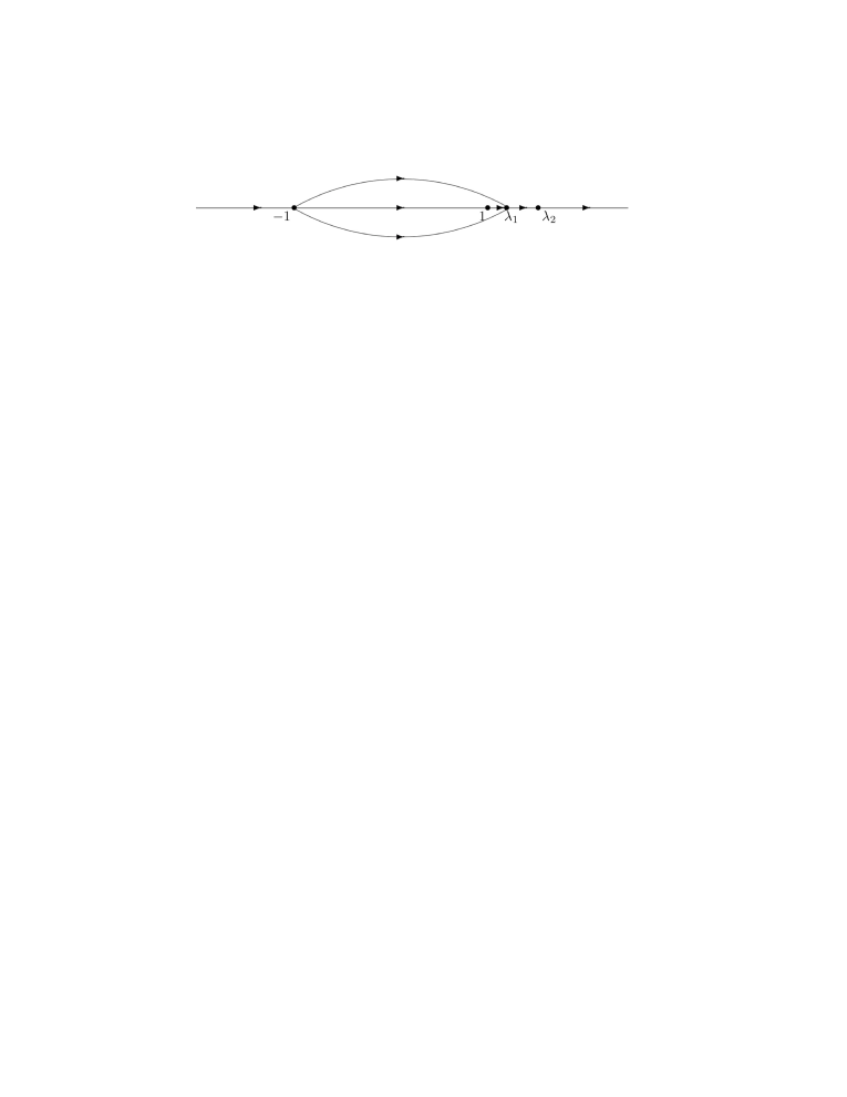
S(z)=\left\{\begin{array}[]{ll}T(z),&\mbox{for $z$ outside the lens,}\\ &\\ T(z)\left(\begin{array}[]{cc}1&0\\ -e^{2n\phi(z)}&1\\ \end{array}\right),&\mbox{for $z$ in the upper lens,}\\ &\\ T(z)\left(\begin{array}[]{cc}1&0\\ e^{2n\phi(z)}&1\\ \end{array}\right),&\mbox{for $z$ in the lower lens,}\end{array}\right.

(3.6)

where the regions are illustrated in Fig.1. Then $S$ satisfies the jump condition

S_{+}(z)=S_{-}(z)J_{S}(z).

(3.7)

Refer to caption — Figure 1: The jump contours and regions for the RH problem for $S$ when $\lambda_{1}>1$ .

For $\lambda_{1}>1$ , we have

J_{S}(z)=\left\{\begin{array}[]{ll}\left(\begin{array}[]{cc}1&\omega_{2}e^{-2n\phi(z)}\\ 0&1\\ \end{array}\right),&z\in(\lambda_{2},+\infty),\\[11.38092pt] \left(\begin{array}[]{cc}1&\omega_{1}e^{-2n\phi(z)}\\ 0&1\\ \end{array}\right),&z\in(\lambda_{1},\lambda_{2}),\\[11.38092pt] \left(\begin{array}[]{cc}0&e^{-2n\phi(z)}\\ -e^{2n\phi(z)}&0\\ \end{array}\right),&z\in(1,\lambda_{1}),\\[11.38092pt] \left(\begin{array}[]{cc}0&1\\ -1&0\\ \end{array}\right),&z\in(-1,1)\\ \left(\begin{array}[]{cc}1&0\\ e^{2n\phi(z)}&1\\ \end{array}\right),&z~{}\mbox{on lens},\\[11.38092pt] \left(\begin{array}[]{cc}1&e^{-2n\phi_{+}(z)}\\ 0&1\\ \end{array}\right),&z\in(-\infty,-1),\end{array}\right.

(3.8)

where the contours are indicated in Fig. 1.
For $\lambda_{1}<1<\lambda_{2}$ , we have

J_{S}(z)=\left\{\begin{array}[]{ll}\left(\begin{array}[]{cc}1&\omega_{2}e^{-2n\phi(z)}\\ 0&1\\ \end{array}\right),&z\in(\lambda_{2},+\infty),\\[11.38092pt] \left(\begin{array}[]{cc}1&\omega_{1}e^{-2n\phi(z)}\\ 0&1\\ \end{array}\right),&z\in(1,\lambda_{2}),\\[11.38092pt] \left(\begin{array}[]{cc}e^{2n\phi_{+}(z)}&\omega_{1}\\ 0&e^{2n\phi_{-}(z)}\\ \end{array}\right),&z\in(\lambda_{1},1),\\[11.38092pt] \left(\begin{array}[]{cc}0&1\\ -1&0\\ \end{array}\right),&z\in(-1,\lambda_{1}),\\[11.38092pt] \left(\begin{array}[]{cc}1&0\\ e^{2n\phi(z)}&1\\ \end{array}\right),&z~{}\mbox{on lens},\\[11.38092pt] \left(\begin{array}[]{cc}1&e^{-2n\phi_{+}(z)}\\ 0&1\\ \end{array}\right),&z\in(-\infty,-1).\end{array}\right.

For $\lambda_{1}<\lambda_{2}<1$ , we have

J_{S}(z)=\left\{\begin{array}[]{ll}\left(\begin{array}[]{cc}1&\omega_{2}e^{-2n\phi(z)}\\ 0&1\\ \end{array}\right),&z\in(1,+\infty),\\[11.38092pt] \left(\begin{array}[]{cc}e^{2n\phi_{+}(z)}&\omega_{2}\\ 0&e^{2n\phi_{-}(z)}\\ \end{array}\right),&z\in(\lambda_{2},1),\\[11.38092pt] \left(\begin{array}[]{cc}e^{2n\phi_{+}(z)}&\omega_{1}\\ 0&e^{2n\phi_{-}(z)}\\ \end{array}\right),&z\in(\lambda_{1},\lambda_{2}),\\[11.38092pt] \left(\begin{array}[]{cc}0&1\\ -1&0\\ \end{array}\right),&z\in(-1,\lambda_{1}),\\[11.38092pt] \left(\begin{array}[]{cc}1&0\\ e^{2n\phi(z)}&1\\ \end{array}\right),&z~{}\mbox{on lens},\\[11.38092pt] \left(\begin{array}[]{cc}1&e^{-2n\phi_{+}(z)}\\ 0&1\\ \end{array}\right),&z\in(-\infty,-1).\end{array}\right.

3.3 Global Parametrix

The global parametrix solves the following approximating RH problem, with the jump along $(-1,\lambda_{1})$ :

(a) $N(z)$ is analytic in $\mathbb{C}\backslash[-1,\lambda_{1}]$ ;

(b)

N_{+}(x)=N_{-}(x)\left(\begin{array}[]{cc}0&1\\ -1&0\\ \end{array}\right),\quad x\in(-1,\lambda_{1});

(3.9)

(c)

N(z)=I+O(z^{-1}),\quad z\rightarrow\infty.

(3.10)

The solution of the RH problem is constructed explicitly ( see [26] ):

N(z)=\left(\begin{array}[]{cc}\frac{\eta(z)+\eta^{-1}(z)}{2}&\frac{\eta(z)-\eta^{-1}(z)}{2i}\\ -\frac{\eta(z)-\eta^{-1}(z)}{2i}&\frac{\eta(z)+\eta^{-1}(z)}{2}\\ \end{array}\right),\quad\eta(z)=\left(\frac{z-\lambda_{1}}{z+1}\right)^{1/4},

(3.11)

where the branch is chosen such that $\eta(z)$ is analytic in $\mathbb{C}\setminus[-1,\lambda_{1}]$ , and $\eta(z)\sim 1$ as $z\to\infty$ .

3.4 Local parametrix near $z=1$

The jump matrices for $S(z)$ are not close to the identity matrix near the node points $z=\pm 1$ . Thus, local parametrices have to be constructed in the neighborhoods of $z=\pm 1$ . Near $z=-1$ , the parametrix $P^{(-1)}(z)$ can be constructed in terms of the Airy function [9, 11]. We proceed to find a local parametrix $P^{(1)}(z)$ in $U(1,r)$ , which is an open disc centered at $z=1$ with radius $r>0$ . The parametrix solves the following RH problem:

Riemann-Hilbert problem for $P^{(1)}$

(a) $P^{(1)}(z)$ is analytic in $U(1,r)\backslash\Sigma_{S}$ ;

(b) On $\Sigma_{S}\cap U(1,r)$ , $P^{(1)}(z)$ satisfies the same jump condition as $S(z)$ ,

P^{(1)}_{+}(z)=P^{(1)}_{-}(z)J_{S},~{}~{}z\in\Sigma_{S}\cap U(1,r);

(3.12)

P^{(1)}(z)N^{-1}(z)=I+O\left(n^{-1/3}\right);

(3.13)

(d) The behavior of $P^{(1)}(z)=O(\ln(z-\lambda_{k})$ as $z\to\lambda_{k}$ for $k=1,2$ .

To construct the local parametrix, we introduce the following model RH problem, which shares the same jump condition as $P^{(1)}(z)e^{-n\phi(z)\sigma_{3}}$ .

The Riemann-Hilbert problem for $\Psi$

Figure 2: The jump contours and regions for the RH problem for

\Psi

for

s>0

(a) $\Psi(\zeta;x,s)$ ( $\Psi(\zeta)$ , for short) is analytic in $\mathbb{C}\backslash\bigcup_{j=0}^{4}\Sigma_{j}$ , where the jump contours are indicated in Fig. 2;

(b) $\Psi(\zeta)$ satisfies the jump condition for $s>0$

\displaystyle\Psi_{+}(\zeta)=\Psi_{-}(\zeta)\left\{\begin{array}[]{ll}\left(\begin{array}[]{cc}1&\omega_{2}\\ 0&1\\ \end{array}\right),&\zeta\in(s,+\infty),\\[11.38092pt] \left(\begin{array}[]{cc}1&\omega_{1}\\ 0&1\\ \end{array}\right),&\zeta\in(0,s),\\[11.38092pt] \left(\begin{array}[]{cc}1&0\\ 1&1\\ \end{array}\right),&\zeta\in{\Sigma}_{2},\\[11.38092pt] \left(\begin{array}[]{cc}0&1\\ -1&0\\ \end{array}\right),&\zeta\in{\Sigma}_{3},\\[11.38092pt] \left(\begin{array}[]{cc}1&0\\ 1&1\\ \end{array}\right),&\zeta\in\Sigma_{4};\end{array}\right.

(3.29)

\Psi(\zeta)=\left(\begin{array}[]{cc}1&0\\ ir(x,s)&1\end{array}\right)\left[I+\frac{\Psi_{1}(x,s)}{\zeta}+O\left(\zeta^{-2}\right)\right]\zeta^{-\frac{1}{4}\sigma_{3}}\frac{I+i\sigma_{1}}{\sqrt{2}}e^{-(\frac{2}{3}\zeta^{3/2}+x\zeta^{1/2})\sigma_{3}},

(3.30)

where $r(x,s)=i(\Psi_{1}(x,s))_{12}$ .

(d) As $\zeta\rightarrow 0$ ,

\Psi(\zeta)=\Psi^{(0)}(\zeta)\left(I+\frac{1-\omega_{1}}{2\pi i}\left(\begin{array}[]{cc}0&1\\ 0&0\end{array}\right)\ln\zeta\right)E,

(3.31)

where $\Psi^{(0)}(\zeta)$ is analytic at $\zeta=0$ with the expansion

\Psi^{(0)}(\zeta)=\hat{P_{0}}(x,s)(I+\hat{P}_{1}(x,s)\zeta+O(\zeta^{2})).

(3.32)

And the piecewise constant matrix

{E}=\left\{\begin{array}[]{ll}\left(\begin{array}[]{cc}1&0\\ 0&1\end{array}\right),&\zeta\in\Omega_{1},\\ \left(\begin{array}[]{cc}1&0\\ -1&1\end{array}\right),&\zeta\in\Omega_{2},\\ \left(\begin{array}[]{cc}1-\omega_{1}&-\omega_{1}\\ 1&1\end{array}\right),&\zeta\in\Omega_{3},\\ \left(\begin{array}[]{cc}1&-\omega_{1}\\ 0&1\end{array}\right),&\zeta\in\Omega_{4}.\end{array}\right.

(e) As $\zeta\rightarrow s$ ,

\Psi(\zeta)=\Psi^{(1)}(\zeta)\left(I+\frac{\omega_{1}-\omega_{2}}{2\pi i}\left(\begin{array}[]{cc}0&1\\ 0&0\end{array}\right)\ln(\zeta-s)\right)\widehat{E},

(3.33)

where $\Psi^{(1)}(\zeta)$ is analytic at $\zeta=s$ with the following expansion

\Psi^{(1)}(\zeta)=\hat{Q}_{0}(x,s)(I+\hat{Q}_{1}(x,s)(\zeta-s)+O((\zeta-s)^{2})).

(3.34)

Here, the piecewise constant matrix

\widehat{E}=\left\{\begin{array}[]{ll}\left(\begin{array}[]{cc}1&0\\ 0&1\end{array}\right),&\mathop{\rm Im}\nolimits\zeta>0,\\ \left(\begin{array}[]{cc}1&-\omega_{2}\\ 0&1\end{array}\right),&\mathop{\rm Im}\nolimits\zeta<0.\end{array}\right.

The RH problem for $\Psi$ appears recently in the studies of the Fredholm determinants of Painlevé II kernel and Painlevé XXXIV kernel in [27] by the second author of the present work and Dai. It also arises in the studies of the determinants of the Airy kernel with several discontinuities in [8] by Claeys and Doeraene, when the number of discontinuities therein equals to two. The existence of solution to the RH problem for $\Psi$ is proved. It is also shown that $\Psi(\zeta;x,s)$ satisfies the following Lax pair

	$\displaystyle\Psi_{\zeta}(\zeta;x,s)=\left(\begin{array}[]{cc}\frac{v_{1x}}{2\zeta}+\frac{v_{2x}}{2(\zeta-s)}&i-\frac{iv_{1}}{\zeta}-\frac{iv_{2}}{\zeta-s}\\ -i\left(\zeta+x+v_{1}+v_{2}+\frac{v_{1x}^{2}}{4v_{1}\zeta}+\frac{v_{2x}^{2}}{4v_{2}(\zeta-s)}\right)&-\frac{v_{1x}}{2\zeta}-\frac{v_{2x}}{2(\zeta-s)}\end{array}\right)\Psi(\zeta;x,s),$		(3.37)
	$\displaystyle\Psi_{x}(\zeta;x,s)=\left(\begin{array}[]{cc}0&i\\ -i\zeta-2i(v_{1}+v_{2}+\tfrac{x}{2})&0\end{array}\right)\Psi(\zeta;x,s).$		(3.40)

The compatibility condition of the Lax pair is described by the coupled Painlevé II system (1.31). Moreover, the Hamiltonian (1.32) is related to the coefficient of $1/\zeta$ in the large- $\zeta$ expansion of $\Psi(\zeta)$ in (3.30) by

H_{\texttt{II}}(x;s)=\frac{x^{2}}{4}+r(x,s);

(3.41)

see [27, Equation (4.21)].

We introduce the conformal mapping

f(z)=\left(\frac{3}{2}\phi(z)\right)^{2/3}=2(z-1)+\frac{1}{5}(z-1)^{2}+O\left((z-1)^{3}\right),

(3.42)

from a neighborhood of $z=1$ to that of the origin. Then the local parametrix ${P}^{(1)}(z)$ can be constructed for $z\in U(1,r)$ as follows

P^{(1)}(z)=E(z)\Psi\left(n^{2/3}(f(z)-f(\lambda_{1}));n^{2/3}f(\lambda_{1}),n^{2/3}(f(\lambda_{2})-f(\lambda_{1}))\right)e^{n\phi(z)\sigma_{3}},

(3.43)

and the pre-factor

E(z)=N(z)\frac{1}{\sqrt{2}}(I-i\sigma_{1})\left[n^{2/3}(f(z)-f(\lambda_{1}))\right]^{\sigma_{3}/4}\left(\begin{array}[]{cc}1&0\\ -iH_{\texttt{II}}(n^{2/3}f(\lambda_{1});n^{2/3}(f(\lambda_{2})-f(\lambda_{1})))&1\end{array}\right),

(3.44)

where $H_{\texttt{II}}(x;t)$ is the Hamiltonian given in (1.32) and related to the coefficient of $1/\zeta$ in the large- $\zeta$ expansion of $\Psi(\zeta)$ by (3.41).

Proposition 5.

For

\lambda_{k}=\frac{s_{k}}{\sqrt{2n}}=1+\frac{t_{k}}{2n^{2/3}}

with bounded real parameters $t_{k}$ , $k=1,2$ , the local parametrix defined in (3.43) and (3.44) solves the RH problem for $P^{(1)}$ . Moreover, we have the expansion for $z\in\partial U(1,r)$ :

P^{(1)}(z)N(z)^{-1}=I+\frac{\Delta(z)}{n^{1/3}}+O(n^{-2/3}),

(3.45)

where

\Delta(z)=\frac{H_{\texttt{II}}(n^{2/3}f(\lambda_{1});n^{2/3}(f(\lambda_{2})-f(\lambda_{1})))}{2(f(z)-f(\lambda_{1}))^{1/2}}N(z)(\sigma_{3}-i\sigma_{1})N^{-1}(z)=O(1),

(3.46)

and $H_{\texttt{II}}(x,t)$ is the Hamiltonian defined in (1.32).

Proof.

Taking the principle branch for the fractional power, it follows from (3.42) that

(f(x)-f(\lambda_{1}))^{\frac{1}{4}}_{+}=(f(x)-f(\lambda_{1}))^{\frac{1}{4}}_{-}~{}e^{\frac{\pi}{2}i},\quad x<\lambda_{1}.

This, together with the expression of $N(z)$ in (3.11), implies that $E(z)$ is analytic for z in $U(1,r)$ . Recalling the properties of $\Psi(\zeta)$ in (3.29)-(3.33), it is then seen that the jump condition and the local behaviors near $\lambda_{k},k=1,2$ , in the Riemann-Hilbert problem for $P^{(1)}$ , are fulfilled.

We then proceed to check the matching condition (3.13). Substituting the large- $\zeta$ behavior of $\Psi(\zeta)$ (3.30) into (3.43) leads us to the expansion for $z$ on $\partial U(1,r)$ as $n\to\infty$ :

$\displaystyle P^{(1)}(z)N(z)^{-1}$	$\displaystyle=N(z)\frac{1}{\sqrt{2}}(I-i\sigma_{1})\left[n^{2/3}(f(z)-f(\lambda_{1}))\right]^{\sigma_{3}/4}\left(\begin{array}[]{cc}1&0\\ -\frac{i}{4}(n^{2/3}f(\lambda_{1}))^{2}&1\end{array}\right)$	(3.49)
	$\displaystyle~{}~{}\left(I+\frac{\Psi_{1}(n^{2/3}f(\lambda_{1}),n^{2/3}(f(\lambda_{2})-f(\lambda_{1})))}{n^{2/3}(f(z)-f(\lambda_{1}))}+O(n^{-4/3})\right)$
	$\displaystyle~{}~{}\left[n^{2/3}(f(z)-f(\lambda_{1}))\right]^{-\sigma_{3}/4}\frac{1}{\sqrt{2}}(I+i\sigma_{1})e^{n\rho(z;\lambda_{1})\sigma_{3}}N(z)^{-1},$	(3.50)

where

$\displaystyle\rho(z;\lambda_{1})$	$\displaystyle=\frac{2}{3}f(z)^{3/2}-\frac{2}{3}(f(z)-f(\lambda_{1}))^{3/2}-f(\lambda_{1})(f(z)-f(\lambda_{1}))^{1/2}$
	$\displaystyle=\frac{1}{\left(f(z)-f(\lambda_{1})\right)^{1/2}}\left(\frac{2}{3}f(z)^{2}\left(1-\frac{f(\lambda_{1})}{f(z)}\right)^{1/2}-\frac{2}{3}f(z)^{2}\left(1-\frac{f(\lambda_{1})}{f(z)}\right)^{2}\right.$
	$\displaystyle~{}~{}~{}~{}~{}~{}~{}~{}~{}~{}~{}~{}~{}~{}~{}~{}~{}~{}~{}~{}~{}~{}~{}~{}~{}~{}~{}~{}~{}~{}~{}~{}~{}\left.-f(z)f(\lambda_{1})\left(1-\frac{f(\lambda_{1})}{f(z)}\right)\right)$
	$\displaystyle=\frac{f(\lambda_{1})^{2}}{4\left(f(z)-f(\lambda_{1})\right)^{1/2}}(1+O(f(\lambda_{1})).$	(3.51)

Here $f(\lambda_{1})\sim 2(\lambda_{1}-1)$ as $\lambda_{1}\to 1$ . Inserting the definition of $\Psi_{1}$ in (3.30) and (3) into (3.49), we obtain (3.45). For $z\in\partial U(1,r)$ , the denominator in (3.46), namely $f(z)-f(\lambda_{1})$ , is bounded away from zero. It follows from Proposition 1 and (1.36), $H(x;s)$ is analytic for real variables $x$ and $s$ and thus bounded. Therefore, the factor $\Delta$ defined in (3.46) is bounded for $z\in\partial U(1,r)$ . Thus, we obtain the matching condition (3.13) and complete the proof of Proposition 5. ∎

Remark 4.

The estimate in (3.46) and thus the matching condition (3.13) can be established for more general parameters:

\lambda_{k}=\frac{s_{k}}{\sqrt{2n}}=1+\frac{t_{k}}{2n^{2/3}}

where

-c_{1}\leqslant t_{1}<t_{2}\leqslant c_{2}n^{1/6},\qquad t_{2}-t_{1}\leqslant c_{3},

(3.52)

for any given positive constants $c_{k}$ , $k=1,2,3$ . Actually, for such parameters, we have

n^{2/3}(f(\lambda_{2})-f(\lambda_{1}))=t_{2}-t_{1}+O(n^{-1/3}).

In view of the asymptotic behavior (1.37) and the relation (1.36), we know that $H_{\texttt{II}}(x;s)$ is exponentially small for bounded $s$ and large positive $x$ . Therefore, we have the estimate (3.46) for $d\leqslant t_{1}\leqslant c_{2}n^{1/6}$ with a certain big enough constant $d$ . This, together with the estimate (3.46) derived before for $-c_{1}\leqslant t_{1}\leqslant d$ , leads us to the claim.

3.5 The final transformation: $S\rightarrow R$

The final transformation is defined by

R(z)=\left\{\begin{array}[]{ll}S(z)N^{-1}(z),&z\in\mathbb{C}\backslash\left\{U(-1,r)\cup U(1,r)\cup\Sigma_{S}\right\},\\ S(z)\left\{P^{(-1)}(z)\right\}^{-1},&z\in U(-1,r)\backslash\Sigma_{S},\\ S(z)\left\{P^{(1)}(z)\right\}^{-1},&z\in U(1,r)\backslash\Sigma_{S}.\end{array}\right.

(3.53)

From the matching condition (3.13), we have

\|J_{R}(z)-I\|_{L^{2}\cap L^{\infty}(\Sigma_{R})}=O(n^{-1/3}),

(3.54)

where the error bound is uniform for the parameters $t_{1}$ and $t_{2}$ specified by (3.52). Thus, by a standard argument as given in [9, 10, 11], we have the estimate

R(z)=I+O(n^{-1/3}),

(3.55)

where the error bound is uniform for $z$ in whole complex plane.

4 Proofs of Theorem 2-4

In this section, we will prove the main results on the asymptotics of the Hankel determinants and several quantities related to the orthogonal polynomials, including the recurrence coefficients and the leading coefficients. Moreover, we will derive the asymptotics of the coupled Painlevé IV system.

4.1 Proof of Theorem 2: asymptotic of the Hankel determinants

Lemma 1.

Let

s_{k}=\sqrt{2n}+\frac{t_{k}}{2n^{1/6}},\quad k=1,2,

and $F(s_{1},s_{2})$ be the logarithmic derivative of the Hankel determinant defined in (1.20), we have

F(s_{1},s_{2})=\sqrt{2}n^{1/6}H_{\texttt{II}}(t_{1};t_{2}-t_{1})+O(n^{-1/6}),

(4.1)

where $H_{\texttt{II}}(x;s)$ is the Hamiltonian for the coupled Painlevé II system as defined in (1.32). The error bound is uniform for $-c_{1}\leqslant t_{1}<t_{2}\leqslant c_{2}n^{1/6}$ and $t_{2}-t_{1}\leqslant c_{3}$ for any given positive constants $c_{k}$ , $k=1,2,3$ ; see also (3.52).

Proof.

Tracing back the series of invertible transformations (3.1), (3.6) and (3.53)

Y\to T\to S\to R,

we have

Y_{+}(\sqrt{2n}z)=(2n)^{\frac{1}{2}n\sigma_{3}}e^{\frac{1}{2}nl\sigma_{3}}R(z)E(z)\Psi_{+}\left(n^{2/3}(f(z)-f(\lambda_{1}));x_{n},s_{n}\right)e^{nz^{2}\sigma_{3}},\quad\lambda_{1}<z<1+r,

(4.2)

where $E(z)$ as defined in (3.44) is analytic for $|z-1|<r$ . With the parameters specified by (3.52), we have

x_{n}=n^{2/3}f(\lambda_{1})=t_{1}+O(n^{-1/3}),\quad s_{n}=n^{2/3}(f(\lambda_{2})-f(\lambda_{1}))=t_{2}-t_{1}+O(n^{-1/3}).

(4.3)

Thus, substituting (4.2) and the estimate (3.55) into the differential identity (2.3), we obtain

\displaystyle F(s_{1},s_{2})=\frac{1-\omega_{1}}{\sqrt{2}\pi i}n^{1/6}\left(\Psi^{-1}\Psi_{\zeta}\right)_{21}(0)+\frac{\omega_{1}-\omega_{2}}{\sqrt{2}\pi i}n^{1/6}\left(\Psi^{-1}\Psi_{\zeta}\right)_{21}(s_{n})+O(n^{-1/6}),

(4.4)

where the error bound is uniform for $s_{1}$ and $s_{2}$ specified by (3.52). Using the expansions of $\Psi(z)$ near $z=0$ and $z=s$ in (3.31) and (3.33), we have

\displaystyle F(s_{1},s_{2})=\frac{1-\omega_{1}}{\sqrt{2}\pi i}n^{1/6}(\hat{P}_{1})_{21}(x_{n},s_{n})+\frac{\omega_{1}-\omega_{2}}{\sqrt{2}\pi i}n^{1/6}(\hat{Q}_{1})_{21}(x_{n},s_{n})+O(n^{-1/6}),

(4.5)

where $\hat{P}_{1}$ and $\hat{Q}_{1}$ are defined in (3.32) and (3.34), respectively.

Next, we express $\hat{P}_{1}$ and $\hat{Q}_{1}$ in terms of the coupled Painlevé II system. Applying the differential equation (3.37), we obtain

	$\displaystyle\frac{1-\omega_{1}}{2\pi i}\hat{P}_{0}\left(\begin{array}[]{cc}0&1\\ 0&0\end{array}\right)\hat{P}_{0}^{-1}=\left(\begin{array}[]{cc}\frac{v_{1x}}{2}&-iv_{1}\\ -i\frac{v_{1x}^{2}}{4v_{1}}&-\frac{v_{1x}}{2}\end{array}\right),$		(4.10)
	$\displaystyle\hat{P}_{1}+\frac{1-\omega_{1}}{2\pi i}\left[\hat{P}_{1},\left(\begin{array}[]{cc}0&1\\ 0&0\end{array}\right)\right]=\hat{P}_{0}^{-1}\left(\begin{array}[]{cc}-\frac{v_{2x}}{2s}&i+\frac{iv_{2}}{s}\\ -i\left(x+v_{1}+v_{2}-\frac{v_{2x}^{2}}{4v_{2}s}\right)&\frac{v_{2x}}{2s}\end{array}\right)\hat{P}_{0}.$		(4.15)

Now

\hat{P}_{0}\left(\begin{array}[]{cc}0&1\\ 0&0\end{array}\right)\hat{P}_{0}^{-1}=\left(\begin{array}[]{cc}-(\hat{P}_{0})_{11}(\hat{P}_{0})_{21}&(\hat{P}_{0})_{11}^{2}\\ -(\hat{P}_{0})_{21}^{2}&(\hat{P}_{0})_{11}(\hat{P}_{0})_{21}\\ \end{array}\right).

Then, this, together with (4.10), leads us to

\frac{1-\omega_{1}}{2\pi i}(\hat{P}_{0})_{11}^{2}=-iv_{1},\quad\frac{1-\omega_{1}}{2\pi i}(\hat{P}_{0})_{21}^{2}=i\frac{v_{1x}^{2}}{4v_{1}},\quad\frac{1-\omega_{1}}{2\pi i}(\hat{P}_{0})_{11}(\hat{P}_{0})_{21}=-\frac{v_{1x}}{2}.

(4.16)

From the $(21)$ entry of the matrix equation (4.15), it is seen that

(\hat{P}_{1})_{21}=-i\left(x+v_{1}+v_{2}-\frac{v_{2x}^{2}}{4v_{2}s}\right)(\hat{P_{0}})_{11}^{2}+\frac{v_{2x}}{s}(\hat{P}_{0})_{11}(\hat{P}_{0})_{21}+i\left(1+\frac{v_{2}}{s}\right)(\hat{P_{0}})_{21}^{2}.

(4.17)

Substituting (4.16) into (4.17), we obtain

\frac{1-\omega_{1}}{\pi i}(\hat{P}_{1})_{21}=-2v_{1}\left(x+v_{1}+v_{2}-\frac{v_{2x}^{2}}{4v_{2}s}\right)-\frac{v_{1x}v_{2x}}{s}+\left(1+\frac{v_{2}}{s}\right)\frac{v_{1x}^{2}}{2v_{1}}.

(4.18)

Similarly, we have that

\frac{\omega_{1}-\omega_{2}}{2\pi i}(\hat{Q}_{0})_{11}^{2}=-iv_{2},\quad\frac{\omega_{1}-\omega_{2}}{2\pi i}(\hat{Q}_{0})_{21}^{2}=i\frac{v_{2x}^{2}}{4v_{2}},

(4.19)

and

\frac{\omega_{1}-\omega_{2}}{\pi i}(\hat{Q}_{1})_{21}=-2v_{2}\left(x-s+v_{1}+v_{2}+\frac{v_{1x}^{2}}{4v_{1}s}\right)+\frac{v_{1x}v_{2x}}{s}-\left(1-\frac{v_{1}}{s}\right)\frac{v_{2x}^{2}}{2v_{2}}.

(4.20)

Therefore, we obtain from (1.31), (4.3) (4.5), (4.18) and (4.20) that

$\displaystyle F(s_{1},s_{2})$	$\displaystyle=\frac{1}{\sqrt{2}}n^{1/6}\left(-2v_{2}s_{n}-2(v_{1}+v_{2})(x_{n}+v_{1}+v_{2})+\frac{v_{1x}^{2}}{2v_{1}}+\frac{v_{2x}^{2}}{2v_{2}}\right)+O(n^{-1/6})$	(4.21)
	$\displaystyle=\sqrt{2}n^{1/6}H_{\texttt{II}}(x_{n};s_{n})+O(n^{-1/6})$	(4.22)
	$\displaystyle=\sqrt{2}n^{1/6}H_{\texttt{II}}(t_{1};t_{2}-t_{1})+O(n^{-1/6}),$	(4.23)

where $H_{\texttt{II}}(x;s)$ is the Hamiltonian for the coupled Painlevé II system as defined in (1.32). This completes the proof Lemma 1. ∎

Next we derive the asymptotic expansion for the Hankel determinant $D_{n}$ defined by (1) when the jump discontinuities of the weight function (1.5) are large enough.

Lemma 2.

For $s_{2}>s_{1}\geqslant\sqrt{2n}+c_{0}$ and any given positive constant $c_{0}$ , we have the asymptotic approximation for the Hankel determinant $D_{n}(s_{1},s_{2})=D_{n}(s_{1},s_{2};\omega_{1},\omega_{2})$ defined by (1)

D_{n}(s_{1},s_{2})=D_{n}^{\texttt{GUE}}\left(1+O\left(e^{-cn^{1/4}}\right)\right),

(4.24)

where $c$ is some positive constant and $D_{n}^{\texttt{GUE}}$ , given explicitly in (1.6), is the Hankel determinant associated with the pure Gaussian weight.

Proof.

For $s_{2}>s_{1}\geqslant\sqrt{2n}+c_{0}$ , we have $\lambda_{2}>\lambda_{1}\geqslant 1+\frac{c_{0}}{\sqrt{2n}}>1$ . On account of (3.42), there is some constant $c>0$ such that

n\phi(\lambda)>cn^{1/4}

for $\lambda>\lambda_{1}$ . Thus, the jump matrices $J_{S}(z)$ defined in (3.8) tend to the identity matrix exponentially fast for $z\in(\lambda_{1},\lambda_{2})\cup(\lambda_{2},+\infty)$ . Therefore, we have

S(z)=(I+O(e^{-2n\phi(\lambda_{1})})S_{0}(z),

(4.25)

where $S_{0}(z)$ is solution to the RH problem for $S$ when the parameters $\omega_{1}=\omega_{2}=1$ and $\lambda_{1}=1$ therein. Tracing back the sequence of transformations $Y\to T\to S$ , given in (3.1), (3.6), we have

Y(\sqrt{2n}z)=(2n)^{\frac{1}{2}n\sigma_{3}}e^{\frac{1}{2}nl\sigma_{3}}(I+O(e^{-2n\phi(\lambda_{1})})S_{0}(z)e^{ng(z)\sigma_{3}-\frac{1}{2}nl\sigma_{3}},

(4.26)

where $e^{ng(z)\sigma_{3}}=(I+O\left(\frac{1}{z^{2}}\right))z^{n\sigma_{3}}$ . In view of (2.2) and the differential identity (2.4), we obtain

F(s_{1},s_{2})=2p_{n}+O\left(e^{-2n\phi(\lambda_{1})}\right)=O\left(e^{-2n\phi(\lambda_{1})}\right),

(4.27)

where $p_{n}=0$ is the sub-leading coefficient of the monic Hermite polynomial of degree $n$ . We integrate on both sides of the above equation and obtain

\ln D_{n}(s_{1},s_{2})-\ln D_{n}(s_{1}+L,s_{2}+L)=\int_{s_{1}}^{L+s_{1}}O\left(e^{-2n\phi(\lambda_{1})}\right)d\tau.

(4.28)

Let $L\to+\infty$ , we get (4.24) and complete the proof of Lemma 2. ∎

Now, we are ready to prove Theorem 2. Integrating on both sides of the equation (4.1), we obtain for some positive constant $c_{0}$ that

\ln D_{n}(s_{1},s_{2})-\ln D_{n}(s_{1}+c_{0},s_{2}+c_{0})=-\int_{t_{1}}^{t_{0}}H_{\texttt{II}}(\tau;t_{2}-t_{1})d\tau+O(n^{-1/6}),

(4.29)

where

s_{1}=\sqrt{2n}+\frac{t_{1}}{\sqrt{2}n^{1/6}},\quad s_{2}=\sqrt{2n}+\frac{t_{2}}{\sqrt{2}n^{1/6}}

for $t_{k}$ , $k=1,2$ , in any compact subset of $\mathbb{R}$ and

t_{0}=n^{2/3}f(\frac{s_{1}+c_{0}}{\sqrt{2n}})\sim\sqrt{2}c_{0}n^{1/6}.

(4.30)

In view of (4.24), we have

\ln D_{n}(s_{1}+c_{0},s_{2}+c_{0})=D_{n}^{\texttt{GUE}}\left(1+O\left(e^{-cn^{1/4}}\right)\right),

(4.31)

where $c$ is some positive constant and $D_{n}^{\texttt{GUE}}$ is the Hankel determinant associated with the Gaussian weight; see (1.6). Recalling (1.36), we obtain from an integration by parts that

\int_{t_{1}}^{t_{0}}H_{\texttt{II}}(\tau;t_{2}-t_{1})d\tau=\int_{t_{1}}^{t_{0}}(\tau-t_{1})\left(u_{1}(\tau;t_{2}-t_{1})^{2}+u_{2}(\tau;t_{2}-t_{1})^{2}\right)d\tau,

(4.32)

where $u_{1}(x)$ and $u_{2}(x)$ are solutions to the coupled nonlinear differential equations (1.34) subject to the boundary conditions (1.37) as $x\to+\infty$ . On account of (1.37) and (4.30), we have

\int_{t_{0}}^{+\infty}(\tau-t_{1})\left(u_{1}(\tau;t_{2}-t_{1})^{2}+u_{2}^{2}(\tau;t_{2}-t_{1})\right)d\tau=O\left(e^{-cn^{1/4}}\right),

(4.33)

for some constant $c>0$ . Inserting (4.31) and (4.33) into (4.29), we obtain (1.38). This completes the proof of Theorem 2.

4.2 Proof of theorem 3: asymptotics of the coupled Painlevé IV

From this section, the parameters in (1.5) are defined by $s_{1}=\sqrt{2n}\lambda_{1}=\sqrt{2n}+\frac{t_{1}}{\sqrt{2}n^{1/6}}$ and $s_{2}=\sqrt{2n}\lambda_{2}=\sqrt{2n}+\frac{t_{2}}{\sqrt{2}n^{1/6}},$ with $t_{1}$ and $t_{2}$ in any compact subset of $\mathbb{R}$ . Tracing back the sequence of transformations $Y\to T\to S\to R$ , given in (3.1), (3.6) and (3.53), we have the expression for large $z$ :

Y(\sqrt{2n}z)=(2n)^{\frac{1}{2}n\sigma_{3}}e^{\frac{1}{2}nl\sigma_{3}}R(z)N(z)e^{ng(z)\sigma_{3}-\frac{1}{2}nl\sigma_{3}},

(4.34)

where $l=-1-2\ln 2$ . From the definition of $g(z)$ in (3.2), it is seen that

e^{ng(z)\sigma_{3}}z^{-n\sigma_{3}}=I+O\left(\frac{1}{z^{2}}\right),\quad z\to\infty.

By the expression of $N(z)$ in (3.11), we have the expansion

N(z)=I+\frac{N_{1}}{z}+O\left(\frac{1}{z^{2}}\right),\quad z\to\infty,

(4.35)

where $N_{1}=-\frac{1}{4}(1+\lambda_{1})\sigma_{2}$ . It follows from the expansion of the jump for $R(z)$ in (3.45) and (3.46) that

R(z)=I+\frac{R^{(1)}(z)}{n^{1/3}}+O\left(\frac{1}{n^{2/3}}\right),\quad n\rightarrow\infty.

(4.36)

Here, $R^{(1)}$ satisfy the jump relation

R^{(1)}_{+}(z)-R^{(1)}_{-}(z)=\Delta(z),

(4.37)

where $\Delta(z)$ is given in (3.46) and $R^{(1)}(z)=O(1/z)$ for $z$ large. Applying Cauchy’s theorem, it is seen that

R^{(1)}(z)=\left\{\begin{array}[]{ll}\frac{\sqrt{1+\lambda_{1}}H_{\texttt{II}}(n^{2/3}f(\lambda_{1});n^{2/3}(f(\lambda_{2})-f(\lambda_{1})))}{2\sqrt{f^{\prime}(\lambda_{1})}(z-\lambda_{1})}(\sigma_{3}-i\sigma_{1})-\Delta(z),&z\in U(1,r),\\[8.5359pt] \frac{\sqrt{1+\lambda_{1}}H_{\texttt{II}}(n^{2/3}f(\lambda_{1});n^{2/3}(f(\lambda_{2})-f(\lambda_{1})))}{2\sqrt{f^{\prime}(\lambda_{1})}(z-\lambda_{1})}(\sigma_{3}-i\sigma_{1}),&z\not\in\overline{U(1,r)}.\end{array}\right.

(4.38)

Thus, we get from the expression the following expansion as $z\to\infty$

R(z)=I+\frac{R_{1}}{z}+O\left(\frac{1}{z^{2}}\right),

(4.39)

and

	$\displaystyle R_{1}$	$\displaystyle=\frac{\sqrt{1+\lambda_{1}}}{2\sqrt{f^{\prime}(\lambda_{1})}n^{1/3}}H_{\texttt{II}}(n^{2/3}f(\lambda_{1});n^{2/3}(f(\lambda_{2})-f(\lambda_{1})))(\sigma_{3}-i\sigma_{1})$
		$\displaystyle=\frac{1}{2n^{1/3}}H_{\texttt{II}}(t_{1};t_{2}-t_{1})(\sigma_{3}-i\sigma_{1})+O(n^{-2/3}),$		(4.40)

where use is also made of (3.42). In view of (3.11), (3.42) and (3.46), we have the following expansion as $z\to\lambda_{1}$

R^{(1)}(z)=-\frac{1}{10}H_{\texttt{II}}(t_{1};t_{2}-t_{1})(\sigma_{3}-i\sigma_{1})+O(n^{-2/3})+O(z-\lambda_{1}).

(4.41)

Substituting (4.35), (4.39) and (4.2) into (4.34) yields

	$\displaystyle Y_{1}$	$\displaystyle=\sqrt{2n}(2n)^{\frac{1}{2}n\sigma_{3}}e^{\frac{1}{2}nl\sigma_{3}}(R_{1}+N_{1})e^{-\frac{1}{2}nl\sigma_{3}}(2n)^{-\frac{1}{2}n\sigma_{3}}$		(4.42)
		$\displaystyle=\sqrt{2n}(2n)^{\frac{1}{2}n\sigma_{3}}e^{\frac{1}{2}nl\sigma_{3}}\left(-\frac{1}{2}\sigma_{2}+\frac{H_{\texttt{II}}(t_{1};t_{2}-t_{1})}{2n^{1/3}}(\sigma_{3}-i\sigma_{1})+O(n^{-2/3})\right)e^{-\frac{1}{2}nl\sigma_{3}}(2n)^{-\frac{1}{2}n\sigma_{3}}.$		(4.43)

This, together with the relation (2.29), implies that

	$\displaystyle y(x;s)$	$\displaystyle=-2(Y_{1})_{21}e^{-x^{2}}$
		$\displaystyle=i(2n)^{-n+\frac{1}{2}}e^{-x^{2}-nl}\left(1+\frac{H_{II}(t_{1};t_{2}-t_{1})}{n^{1/3}}+O(n^{-2/3})\right),$		(4.44)

where $x=\frac{s_{1}+s_{2}}{2}=\sqrt{2n}+\frac{t_{1}+t_{2}}{2\sqrt{2}n^{1/6}}$ and $s=\frac{s_{2}-s_{1}}{2}=\frac{t_{2}-t_{1}}{2\sqrt{2}n^{1/6}}$ . Recalling $l=-1-2\ln 2$ , we obtain the asymptotic expansion of $y(x;s)$ as given in (1.47).

Next, we consider the asymptotics of $a_{k}(x;s)$ and $a_{k}(x;s)$ for $k=1,2$ . It follows from the mastar equation of the Lax pair (2.18) that

	$\displaystyle a_{1}(x;s)=\frac{1}{y(x;s)}\lim_{z\rightarrow-s}(z+s)(\Phi_{z}\Phi^{-1})_{12},$		(4.45)
	$\displaystyle a_{2}(x;s)=\frac{1}{y(x;s)}\lim_{z\rightarrow s}(z-s)(\Phi_{z}\Phi^{-1})_{12},$		(4.46)
	$\displaystyle b_{1}(x;s)=\frac{1}{a_{1}(x;s)}\lim_{z\rightarrow-s}(z+s)(\Phi_{z}\Phi^{-1})_{11},$		(4.47)
	$\displaystyle b_{2}(x;s)=\frac{1}{a_{2}(x;s)}\lim_{z\rightarrow s}(z-s)(\Phi_{z}\Phi^{-1})_{11},$		(4.48)

where the subscript $z$ denotes the derivative with respect to $z$ . It is seen from (2.12) that

\Phi_{z}\Phi^{-1}=\sigma_{1}e^{\frac{x^{2}}{2}\sigma_{3}}[Y_{z}(z+x)Y^{-1}(z+x)+Y(z+x)(-(z+x)\sigma_{3})Y^{-1}(z+x)]e^{-\frac{x^{2}}{2}\sigma_{3}}\sigma_{1}.

(4.49)

According to (4.45) and (4.49) and in view of the fact that $Y(z)$ has at most logarithm singularity at $s_{1}$ , we have

$\displaystyle a_{1}(x;s)$	$\displaystyle=\frac{1}{y(x;s)}e^{-x^{2}}\lim_{z\rightarrow-s}(z+s)(Y_{z}(z+x)Y^{-1}(z+x))_{21},$
	$\displaystyle=\frac{1}{y(x;s)}e^{-x^{2}}\lim_{z\rightarrow s_{1}}(z-s_{1})(Y_{z}(z)Y^{-1}(z))_{21},$
	$\displaystyle=\frac{1}{y(x;s)}e^{-x^{2}}\lim_{z\rightarrow\lambda_{1}}\sqrt{2n}(z-\lambda_{1})(Y_{z}(\sqrt{2n}z)Y^{-1}(\sqrt{2n}z))_{21}.$	(4.50)

Inserting (4.2) into (4.2), it is seen that

a_{1}(x;s)=\frac{(2n)^{-n}}{y(x;s)}e^{-x^{2}-nl}\left(R(\lambda_{1})E(\lambda_{1})\left(\lim_{\zeta\rightarrow 0}\zeta\Psi_{\zeta}(\zeta)\Psi^{-1}(\zeta)\right)E^{-1}(\lambda_{1})R^{-1}(\lambda_{1})\right)_{21},

(4.51)

where use is made of the fact that $E(z)$ and $R(z)$ are analytic at $z=\lambda_{1}$ . It follows from the behavior of $\Psi(z)$ near $z=\lambda_{1}$ as given in (3.31) that

\lim_{\zeta\rightarrow 0}\zeta\Psi_{\zeta}(\zeta)\Psi^{-1}(\zeta)=\frac{1-\omega_{1}}{2\pi i}\hat{P}_{0}\left(\begin{array}[]{cc}0&1\\ 0&0\end{array}\right)\hat{P}_{0}^{-1}.

(4.52)

From the expression (3.44), we get for $k=1,2$ ,

E(\lambda_{k})=\frac{1}{\sqrt{2}}(I-i\sigma_{1})n^{\sigma_{3}/6}2^{\sigma_{3}/2}\left(\begin{array}[]{cc}1&0\\ -iH_{\texttt{II}}(t_{1};t_{2}-t_{1})&1\end{array}\right)(I+O(n^{-2/3})).

(4.53)

Thus, we obtain from (3.55), (4.51)-(4.53) that

a_{1}(x;s)=\frac{(1-\omega_{1})(2n)^{-n}}{2\pi iy(x;s)}e^{-x^{2}-nl}\\ \left((\hat{P}_{0})_{11}^{2}n^{1/3}+i(\hat{P}_{0})_{11}(\hat{P}_{0})_{21}+H_{\texttt{II}}(t_{1};t_{2}-t_{1})(\hat{P}_{0})_{11}^{2}+O(n^{-1/3})\right).

Using (4.16) and (4.2), we obtain the asymptotic approximation of $a_{1}(x;s)$ as stated in (1.43).

Similarly, from (3.33), (3.43) and (4.46), we have

\displaystyle a_{2}(x;s)

\displaystyle=\frac{(2n)^{-n}}{y(x;s)}e^{-x^{2}-nl}\left(R(\lambda_{2})E(\lambda_{2})\frac{\omega_{1}-\omega_{2}}{2\pi i}\hat{Q}_{0}\left(\begin{array}[]{cc}0&1\\ 0&0\end{array}\right)\hat{Q}_{0}^{-1}E^{-1}(\lambda_{2})R^{-1}(\lambda_{2})\right)_{21}.

(4.56)

Substituting (3.55), (4.19), (4.2) and (4.53) into (4.56), we obtain the asymptotic expansion of $a_{2}(x;s)$ as given in (1.44). In view of (4.47) and (4.48), we obtain the asymptotics of $b_{1}(x;s)$ and $b_{2}(x;s)$ by considering the $(2,2)$ entry of the matrices in (4.51) and (4.56):

	$\displaystyle b_{1}(x;s)$	$\displaystyle=\frac{(1-\omega_{1})}{2\pi ia_{1}(x;s)}\left(-i(\hat{P}_{0})_{11}^{2}n^{1/3}+O(n^{-1/3})\right)$
		$\displaystyle=\sqrt{2n}\left(1-\frac{v_{1x}(t_{1};t_{2}-t_{1})}{2v_{1}(t_{1};t_{2}-t_{1})n^{1/3}}+O(n^{-2/3})\right),\quad n\rightarrow\infty,$		(4.57)

and

	$\displaystyle b_{2}(x;s)$	$\displaystyle=\frac{(\omega_{1}-\omega_{2})}{2\pi ia_{2}(x;s)}\left(-i(\hat{Q}_{0})_{11}^{2}n^{1/3}+O(n^{-1/3})\right)$
		$\displaystyle=\sqrt{2n}\left(1-\frac{v_{2x}(t_{1};t_{2}-t_{1})}{2v_{2}(t_{1};t_{2}-t_{1})n^{1/3}}+O(n^{-2/3})\right),\quad n\rightarrow\infty,$		(4.58)

where $x=\frac{s_{1}+s_{2}}{2}=\sqrt{2n}+\frac{t_{1}+t_{2}}{2\sqrt{2}n^{1/6}}$ and $s=\frac{s_{2}-s_{1}}{2}=\frac{t_{2}-t_{1}}{2\sqrt{2}n^{1/6}}$ . This completes the proof of Theorem 3.

4.3 Proof of Theorem 4: asymptotics of the orthogonal polynomials

From (1.43)-(1.46), we have

a_{1}(x;s)b_{1}(x;s)^{2}=-\sqrt{2}n^{5/6}\left(v_{1}(t_{1};t_{2}-t_{1})-\frac{1}{2}v_{1x}(t_{1};t_{2}-t_{1})n^{-1/3}+O(n^{-2/3})\right),

(4.59)

a_{2}(x;s)b_{2}(x;s)^{2}=-\sqrt{2}n^{5/6}\left(v_{2}(t_{1};t_{2}-t_{1})-\frac{1}{2}v_{2x}(t_{1};t_{2}-t_{1})n^{-1/3}+O(n^{-2/3})\right),

(4.60)

a_{1}(x;s)b_{1}(x;s)+a_{2}(x;s)b_{2}(x;s)=-n^{1/3}\left((v_{1}(t_{1};t_{2}-t_{1})+v_{2}(t_{1};t_{2}-t_{1}))+O(n^{-2/3})\right).

(4.61)

Substituting (4.59)-(4.61) into (1.23), (1.24), (1.27) and (1.28), we obtain the asymptotics of the recurrence coefficients and $\pi_{n}(s_{k})$ , $k=1,2$ , as given in (1.48), (1.49), (1.51) and (1.52), respectively. In view of (2.55), (4.35), (4.2) and (4.43), we derive the asymptotic expansion for the leading coefficient $\gamma_{n-1}$ of the orthonormal polynomial of degree $n-1$ :

$\displaystyle\gamma_{n-1}$	$\displaystyle=\left(-\frac{1}{2\pi i}(Y_{1})_{21}\right)^{1/2}$
	$\displaystyle=\left(\frac{\sqrt{2n}(2n)^{-n}e^{-nl}(R_{1}+N_{1})_{21}}{-2\pi i}\right)^{1/2}$
	$\displaystyle=\frac{2^{\frac{n}{2}-\frac{3}{4}}n^{\frac{1}{4}-\frac{n}{2}}e^{\frac{n}{2}}}{\sqrt{\pi}}\left(1+\frac{H_{\texttt{II}}(t_{1};t_{2}-t_{1}))}{2n^{1/3}}+O(n^{-2/3})\right),\quad n\rightarrow\infty.$	(4.62)

Thus, we complete the proof of Theorem 4.

Acknowledgements

The authors are grateful to Dan Dai for useful comments. Xiao-Bo Wu was partially supported by National Natural Science Foundation of China under grant number 11801376 and Science Foundation of Education Department of Jiangxi Province under grant number GJJ170937. Shuai-Xia Xu was partially supported by National Natural Science Foundation of China under grant numbers 11971492, 11571376 and 11201493.

References

[1] A. Bogatskiy, T. Claeys and A. Its, Hankel determinant and orthogonal polynomials for a Gaussian weight with a discontinuity at the edge, Comm. Math. Phys., 347, 127–162 (2016).
[2] O. Bohigas and M.P. Pato, Missing levels in correlated spectra, Phys. Lett. B , 595 , 171–176 (2004).
[3] O. Bohigas and M.P. Pato, Randomly incomplete spectra and intermediate statistics, Phys. Rev. E (3), 74, 036212 (2006).
[4] F. Bornemann, P. J. Forrester and A. Mays, Finite size effects for spacing distributions in random matrix theory: circular ensembles and Riemann zeros, Stud. Appl. Math. , 138, 401–437 (2017).
[5] C. Charlier and T. Claeys, Thinning and conditioning of the Circular Unitary Ensemble, Random Matrices Theory Appl., 6, no. 2, 1750007 (2017).
[6] C. Charlier and T. Claeys, Large Gap Asymptotics for Airy Kernel Determinants with Discontinuities, Commun. Math. Phys., https://doi.org/10.1007/s00220-019-03538-w (2019).
[7] C. Charlier and A. Deaño, Asymptotics for Hankel determinants associated to a Hermite weight with a varying discontinuity, SIGMA Symmetry Integrability Geom. Methods Appl., 14, Paper No. 018, 43 pp (2018).
[8] T. Claeys and A. Doeraene, The generating function for the Airy point process and a system of coupled Painlevé II equations, Stud. Appl. Math., 140, 403–437 (2018).
[9] P. Deift, Orthogonal polynomials and random matrices: a Riemann-Hilbert approach, Courant Lecture Notes 3, New York University, Amer. Math. Soc., Providence, RI, 1999.
[10] P. Deift, T. Kriecherbauer, K. T.-R. McLaughlin, S. Venakides and X. Zhou, Uniform asymptotics for polynomials orthogonal with respect to varying exponential weights and applications to universality questions in random matrix theory, Comm. Pure Appl. Math., 52, 1335–1425 (1999).
[11] P. Deift, T. Kriecherbauer, K. T.-R. McLaughlin, S. Venakides and X. Zhou, Strong asymptotics of orthogonal polynomials with respect to exponential weights, Comm. Pure Appl. Math., 52, 1491–1552 (1999).
[12] P. Deift and X. Zhou, A steepest descent method for oscillatory Riemann-Hilbert problems, Asymptotics for the MKdV equation, Ann. Math., 137, 295–368 (1993).
[13] A.S. Fokas, A.R. Its, A.A. Kapaev and V.Y. Novokshenov, Painlevé Transcendents: The Riemann–Hilbert Approach, AMS Mathematical Surveys and Monographs, 128, Amer. Math. Soc., Providence, RI, 2006.
[14] A.S. Fokas, A.R. Its and A.V. Kitaev, The isomonodromy approach to matrix models in $2D$ quantum gravity, Comm. Math. Phys., 147, 395–430 (1992).
[15] P.J. Forrester, Log-gases and Random Matrices, London Mathematical Society Monographs Series, 34., Princeton University Press, Princeton, NJ, 2010.
[16] P.J. Forrester and N.S. Witte, Application of the $\tau$ -function theory of Painlevé equations to random matrices: PIV, PII and the GUE, Comm. Math. Phys., 219, 357–398 (2001).
[17] A. Its and I. Krasovsky, Hankel determinant and orthogonal polynomials for the Gaussian weight with a jump, Integrable Systems and Random Matrices, J. Baik et al., eds., Contemp. Math., 458, Amer. Math. Soc., Providence, RI, 2008, 215–247.
[18] M. Jimbo, T. Miwa and K. Ueno, Monodromy preserving deformation of linear ordinary differential equations with rational coefficients II, Phys. D, 2, 407–448 (1981).
[19] H. Kawakami, Four-dimensional Painlevé-type equations associated with ramified linear equations III: Garnier systems and Fuji-Suzuki systerms, SIGMA , 13, 096, 50 pp (2017).
[20] H. Kawakami, Four-dimensional Painlevé-type equations associated with ramified linear equations II: Sasano systems, J. Integrable Syst., 3, no.1, xyy013, 36 pp (2018).
[21] H. Kawakami, A. Nakamura, and H. Sakai, Degeneration scheme of 4-dimensional Painlevé-type equations, arXiv:1209.3836.
[22] C. Min and Y. Chen, Painlevé transcendents and the Hankel determinants generated by a discontinuous Gaussian weight, Math. Methods Appl. Sci., 42, no.1, 301–321 (2019).
[23] M.L. Mehta, Random Matrices, 3rd ed., Elsevier/Academic Press, Amsterdam, 2004.
[24] F.W.J. Olver, A.B. Olde Daalhuis, D.W. Lozier, B.I. Schneider, R.F. Boisvert, C.W. Clark, B.R. Miller and B.V. Saunders, eds, NIST Digital Library of Mathematical Functions, http://dlmf.nist.gov/, Release 1.0.21 of 2018-12-15.
[25] C. Tracy and H. Widom, Level-spacing distributions and the Airy kernel, Comm. Math. Phys., 159, 151–174 (1994).
[26] X.-B. Wu, S.-X. Xu and Y.-Q. Zhao, Gaussian Unitary Ensemble with Boundary Spectrum Singularity and $\sigma$ -Form of the Painlevé II Equation, Stud. Appl. Math., 140, 221–251(2018).
[27] S.-X. Xu and D. Dai, Tracy-Widom distributions in critical unitary random matrix ensembles and the coupled Painlevé II system, Comm. Math. Phys., 365 no. 2, 515–567 (2019).
[28] S.-X. Xu and Y.-Q. Zhao, Painlevé XXXIV asymptotics of orthogonal polynomials for the Gaussian weight with a jump at the edge, Stud. Appl. Math., 127, 67–105 (2011).

Gaussian unitary ensemble with jump discontinuities and the coupled Painlevé II and IV systems

1 Introduction and statement of results

1.1 Statement of results

The coupled Painlevé IV system

Orthogonal polynomials of finite degree: the coupled Painlevé IV system

Theorem 1.

Remark 1.

The coupled Painlevé II system

Proposition 1.

Asymptotics of the Hankel determinants and applications in random matrices

Theorem 2.

Remark 2.

Corollary 1.

Corollary 2.

Asymptotics of the coupled Painlevé IV system

Theorem 3.

Asymptotics of the orthogonal polynomials

Theorem 4.

Remark 3.

1.2 Organization of the rest of this paper

2 Orthogonal polynomials and the coupled Painlevé IV system

2.1 Riemann-Hilbert problem for the orthogonal polynomials

Riemann-Hilbert problem for YY

Proposition 2.

Proof.

Riemann-Hilbert problem for Φ\Phi

2.2 Lax pair and the coupled Painlevé IV system

Proposition 3.

Proof.

Proposition 4.

Proof.

2.3 Proof of Theorem 1

3 Nonlinear steepest descent analysis of the Riemann-Hilbert problem for YY

3.1 The first transformation: Y→TY\rightarrow T

3.2 The second transformation: T→ST\rightarrow S

3.3 Global Parametrix

3.4 Local parametrix near z=1z=1

Riemann-Hilbert problem for P(1)P^{(1)}

The Riemann-Hilbert problem for Ψ\Psi

Proposition 5.

Proof.

Remark 4.

3.5 The final transformation: S→RS\rightarrow R

4 Proofs of Theorem 2-4

4.1 Proof of Theorem 2: asymptotic of the Hankel determinants

Lemma 1.

Proof.

Lemma 2.

Proof.

4.2 Proof of theorem 3: asymptotics of the coupled Painlevé IV

4.3 Proof of Theorem 4: asymptotics of the orthogonal polynomials

Acknowledgements

References

Riemann-Hilbert problem for $Y$

Riemann-Hilbert problem for $\Phi$

3 Nonlinear steepest descent analysis of the Riemann-Hilbert problem for $Y$

3.1 The first transformation: $Y\rightarrow T$

3.2 The second transformation: $T\rightarrow S$

3.4 Local parametrix near $z=1$

Riemann-Hilbert problem for $P^{(1)}$

The Riemann-Hilbert problem for $\Psi$

3.5 The final transformation: $S\rightarrow R$