Gaussian RBF Centered Kernel Alignment (CKA) in the Large Bandwidth Limit

Following the heuristic of [7], we use $\sigma^{\prime}=d_{X}\sigma$ instead of $\sigma$ in Eq. LABEL:eq:kernelOptions when computing the Gram matrix $K_{G(\sigma)}(X)$, where $d_{X}$ is the median distance between examples (rows) of $X$ (e.g., $\sigma=2$ describes a bandwidth equal to twice the median distance between examples). Equivalently, we divide all inter-example distances $|x_{i}-x_{j}|$ by $d_{X}$. This ensures invariance of Gaussian HSIC under isotropic scaling [7].

Our results rely crucially on mean-centering of features in Eqs. 2, 3. Indeed, the analog of Theorem 1 does not hold if, as in [3], features are not centered. This is easy to see by a direct calculation for the example in which feature matrix $X$ is the $2\times 2$ identity and feature matrix $Y$ is a $2\times 2$ of ones, except for a single off-diagonal $0$. Linear CKA equals $3/\sqrt{14}$ in that case, while Gaussian CKA is $1$ for all $\sigma$, as $X$ and $Y$ have identical distance matrices after scaling by the median distances $d_{X}$, $d_{Y}$ as described in the note in section 2.4. Details are provided in the Appendix.

Multiplying by $\sigma^{2}_{X}$, we obtain the connection in Eq. 8 between $\text{HSIC}(K_{G(\sigma)},L)$ and $\text{HSIC}(K_{E},L)$:

An identity analogous to Eq. 8 relates $\text{HSIC}(K_{G(\sigma)},K_{G(\sigma)})$ to its Euclidean version. In the latter case, the higher-order error terms in the HSIC expression are $O(\frac{1}{\sigma^{6}})$ before multiplying by $\sigma^{2}_{X}$, because they result from a product of a $O(\frac{1}{\sigma^{4}})$ error term from one of the two Gaussian Gram matrices with the $O(\frac{1}{\sigma^{2}})$ leading term in the other factor; multiplication by $\sigma^{4}_{X}$ is required to obtain a $O(\frac{1}{\sigma^{2}})$ residual, which will become a $\sigma^{2}_{X}$ factor after taking the square root in the CKA denominator (below).

Lemma 1 follows by dividing the HSIC components described above to form CKA as in Eq. 3:

The case of two Gaussian kernels with bandwidths approaching $\infty$ (whether equal to one another or not) follows by considering one kernel argument at a time, freezing the bandwidth of the other, and using the scalar triangle inequality. Details appear in the Appendix. $\Box$

Theorem 1 follows from Lemma 1 and Corollary 1.

We used sample OpenML data sets [22] (CC BY 4.0 license, https://creativecommons.org/licenses/by/4.0/) for classification (splice, tic-tac-toe, wdbc, optdigits, wine, dna) and regression (cpu, boston, Diabetes(scikit-learn), stock, balloon, cloud); for data sets with multiple versions, we used version 1. These data sets were selected based on two considerations only: smaller size, in order to eliminate the need for GPU acceleration and reduce environmental impact; and an absence of missing values, to simplify the development of internal feature representations for the CKA computations. Data set sizes are given in Table I.

Fully-connected neural networks (NN) with two hidden layers were used. Feature encodings $X$, $Y$ were the sets of activation vectors of the first and second hidden layers, respectively. Alternative NN widths, $w=16,32,64,128,256,512,1024$ were tested, with $w$ and $\frac{w}{4}$ hidden nodes in the first and second hidden layers. A configuration with three hidden layers, of sizes $128,32,8$, was also tested, for which $X$, $Y$ were the activation vectors from layers $1$ and $3$.

NN were trained using the MLPClassifier and MLPRegressor classes in scikit-learn [23], with cross-entropy or quadratic loss for classification and regression, respectively, ReLU activation functions, Glorot-He pseudorandom initialization [24], [25], Adam optimizer [26], learning rate of $0.001$, and a maximum of $2000$ training iterations. CKA was implemented in Python (https://docs.python.org/3/license.html), using NumPy [27] (https://numpy.org/doc/stable/license.html) and Matplotlib [28] (PSF license, https://docs.python.org/3/license.html). Experiments were performed on a workstation with an Intel i9-7920X (12 core) processor and 128GB RAM, under Ubuntu 18.04.5 LTS (GNU public license).

$50$ runs were performed for each pair $(D,w)$ of a data set $D$ and NN width $w$. In each run, a new NN model was trained on the full data set, starting from fresh pseudorandom initial parameter values. A training run was repeated if the resulting in-sample accuracy was below $0.8$ (classification) or if in-sample coefficient of determination was below $0.5$ (regression), but not if the optimization had not converged within the allowed number of iterations. After the network had been trained in a given run, $\text{CKA}_{\text{lin}}$ was computed once, and $\text{CKA}_{G(\sigma)}$ was computed for each bandwidth $\sigma=2^{p},\;p=-4,-3,\cdots,8$, for a total of $50$ $\text{CKA}_{\text{lin}}$ and $650$ $\text{CKA}_{G(\sigma)}$ evaluations per $(D,w)$ pair.

Compute time for the results presented in the paper was approximately $32$ hours, much of it on the $8\cdot 12\cdot(50+650)=67200$ CKA evaluations needed across the $8$ network widths (including the 128-32-8 three-hidden-layer configuration) and the $12$ data sets. Additional runs for validation required another $12$ hours. Several shorter preliminary runs were carried out for debugging and initial selection of the NN hyperparameters; configurations and threshold values were selected empirically in order to ensure a successful end to training after no more than a handful of runs in nearly all cases. Total compute time across all runs is estimated to have been $50$ hours.

CKA means and standard errors (SE = standard deviation divided by $\sqrt{50}$), and medians and standard error equivalent (SE = inter-quartile range divided by $\sqrt{50}$) of the ratio $\rho$ of Eq. 10 were computed across runs. We measured the magnitude of the discrepancy between $\text{CKA}_{G(\sigma)}$ and $\text{CKA}_{\text{lin}}$ by the base-$2$ logarithm of the relative difference between the two measures as in Eq. 11.

Theorem 1 implies that, for large $\sigma$, the logarithmic relative difference of Eq. 11 should decrease along a straight line of slope $-2$ as a function of $\log_{2}\sigma$, reflecting a $O(1/\sigma^{2})$ dependence. Accordingly, for each data set, we determined a $1/\sigma^{2}$ asymptote by extrapolating backward from the largest tested bandwidth value, $\sigma=2^{8}$. If $\sigma<2^{8}$, the predicted relative difference along the $1/\sigma^{2}$ asymptote is as in Eq. 12, where $r_{8}$ is the observed relative difference at $\sigma=2^{8}$.

We determined a $1/\sigma^{2}$ convergence onset bandwidth, $\sigma^{*}_{0}$, as the minimum bandwidth above which the observed $\log_{2}$ relative difference between Gaussian and linear CKA differs by less than $0.25$ from the predicted value along that data set’s $1/\sigma^{2}$ asymptote (Eq. 13).

Threshold values other than $0.25$ in Eq. 13 ($1,0.5,0.1$), corresponding to different tolerances for the log relative difference, yielded similar results in most cases in terms of the resulting relative $\sigma^{*}_{0}$ ranks of the different data sets.

Mean relative difference values between $\text{CKA}_{G(\sigma)}$ and $\text{CKA}_{\text{lin}}$ greater than $0.2$ ($\log_{2}$ values greater than $-2.3$), are observed for several data sets when $\sigma\leq 0.25$ (when $\log_{2}\sigma\leq-2$) in the case of classification; in fact, relative CKA difference values greater than $0.7$ ($\log_{2}\text{ rel.\ CKA diff.}>-0.5$, values in the Appendix) are observed for the dna data set when network width $w$ is $128$ or greater. This shows that noticeably nonlinear behavior of Gaussian CKA is quite possible for small bandwidth values. For some classification data sets, however (wdbc, wine), and most regression data sets, the relative CKA difference remains comparatively small for all bandwidths.

Fig. 1 shows confidence intervals for the means, of radius two standard errors, of the observed $\log_{2}$ relative difference between $\text{CKA}_{G(\sigma)}$ and $\text{CKA}_{\text{lin}}$ as a function of Gaussian bandwidth, $\sigma$ (Eq. 11). Convergence at the rate $1/\sigma^{2}$ for $\sigma\gg 1$ is observed (log-log slope of $-2$ in Fig. 1), as described in Theorem 1. Results are stable across the range of neural network configurations tested. Standard error of the relative CKA difference is observed to decrease as network width increases (e.g., Fig. 2), suggesting that wider networks are less sensitive to variations in initial parameter values.

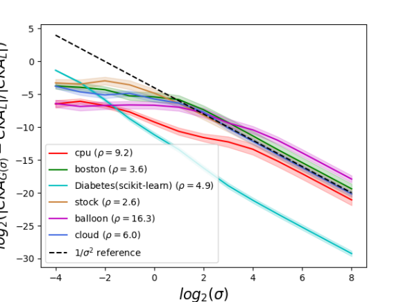
The Diabetes(scikit-learn) data set stands out for having, by far, the smallest mean relative CKA difference among data sets tested, across much of the $\sigma$ range. The neural feature maps $X$ and $Y$ for that data set have nearly proportional linear Gram matrices $K_{\text{lin}}$ and $L_{\text{lin}}$, hence the linear CKA value is very close to $1$. Because the matrix of squared inter-example distances depends linearly on the linear Gram matrix, the Gaussian CKA value is also very close to $1$.

Our experimental results suggest that noticeably nonlinear behavior of Gaussian CKA occurs almost exclusively for bandwidths $\sigma<\rho$. Indeed, for all data sets tested, the observed mean relative difference between linear and Gaussian CKA is less than $0.01$ when $\sigma>\rho$, where $\rho$ is the ratio of maximum to median distance between feature vectors (Eq. 10). This confirms our finding in section 3.2 that $\text{CKA}_{G}(\sigma)$ differs little from $\text{CKA}_{\text{lin}}$ if $\sigma\gg\rho$. Furthermore, our results suggest that the threshold between nonlinear and linear regimes of Gaussian CKA is not substantially less than $\rho$: while mean relative CKA difference for $\sigma\geq 1$ peaked under $0.1$ for two-hidden-layer neural representations, across all data sets tested, relative difference values less than $0.1$ occur for the tic-tac-toe data set in the three-layer 128-32-8 representation only when $\sigma\geq 4$; the lower end of this bandwidth range is quite close to the median $\rho$ value of $4.2$ for that representation (which differs from the width-$64$ two-layer representation in Figs. 1, 2).

We find additional support for the view that $\rho$ approximates the boundary between nonlinear and linear regimes of Gaussian CKA in the fact that the convergence onset bandwidth, $\sigma^{*}_{0}$ (Eq. 13), is largest for the data sets of largest $\rho$: median $\log_{2}\sigma^{*}_{0}=5$, $4$, $4$ for balloon ($\rho\approx 16$), wdbc ($\rho\approx 11$), cpu ($\rho\approx 9$), respectively ($\sigma^{*}_{0}$ and $\rho$ values differ slightly among network widths and depths, but data sets of largest $\rho$ are the same). See Table III. Diabetes(scikit-learn) ties for third with $\log_{2}\sigma^{*}_{0}=4$; median $\log_{2}\sigma^{*}_{0}<4$ for all other data sets. Large differences in $\rho$ between data sets generally translate directly to differences between their $\sigma^{*}_{0}$ values. This is consistent with the analysis in section 3.2, as $\rho$ also controls terms of orders higher than $2$ in the exponential power series.

Our experimental results as a whole confirm $1/\sigma^{2}$ convergence of $\text{CKA}_{G(\sigma)}$ to $\text{CKA}_{\text{lin}}$ as $\sigma\rightarrow\infty$ (Theorem 1), and support the use of the representation eccentricity, $\rho$ (Eq. 10), as a useful heuristic upper bound on the range of bandwidths for which Gaussian CKA can display nonlinear behavior.

References

- [1] C. Cortes, M. Mohri, and A. Rostamizadeh, “Two-stage learning kernel algorithms,” in Proc. 27th Intl. Conf. on Machine Learning, ser. ICML’10. Madison, WI, USA: Omnipress, 2010, p. 239–246.
- [2] ——, “Algorithms for learning kernels based on centered alignment,” J. Mach. Learn. Res., vol. 13, no. 28, pp. 795–828, 2012. [Online]. Available: http://jmlr.org/papers/v13/cortes12a.html
- [3] N. Cristianini, J. Shawe-Taylor, A. Elisseeff, and J. Kandola, “On kernel-target alignment,” in Adv. in Neur. Inf. Proc. Systems, T. Dietterich, S. Becker, and Z. Ghahramani, Eds., vol. 14. MIT Press, 2002. [Online]. Available: https://proceedings.neurips.cc/paper/2001/file/1f71e393b3809197ed66df836fe833e5-Paper.pdf
- [4] T. Górecki, M. Krzyśko, and W. Wołyński, “Independence test and canonical correlation analysis based on the alignment between kernel matrices for multivariate functional data,” Artif Intell Rev, vol. 53, p. 475–499, 2020. [Online]. Available: https://doi.org/10.1007/s10462-018-9666-7
- [5] Y. Lu, L. Wang, J. Lu, J. Yang, and C. Shen, “Multiple kernel clustering based on centered kernel alignment,” Pattern Recognition, vol. 47, no. 11, pp. 3656–3664, 2014. [Online]. Available: https://www.sciencedirect.com/science/article/pii/S0031320314001903
- [6] S. Niazmardi, A. Safari, and S. Homayouni, “A novel multiple kernel learning framework for multiple feature classification,” IEEE J. Sel. Topics Appl. Earth Obs. and Remote Sensing, vol. 10, no. 8, pp. 3734–3743, 2017.
- [7] S. Kornblith, M. Norouzi, H. Lee, and G. E. Hinton, “Similarity of neural network representations revisited,” in Proc. 36th Intl. Conf. Mach. Learn., ICML 2019, 9-15 June 2019, Long Beach, California, USA, ser. Proc. Mach. Learn. Res., K. Chaudhuri and R. Salakhutdinov, Eds., vol. 97. PMLR, 2019, pp. 3519–3529. [Online]. Available: http://proceedings.mlr.press/v97/kornblith19a.html
- [8] F. Ding, J.-S. Denain, and J. Steinhardt, “Grounding representation similarity through statistical testing,” in Thirty-Fifth Conference on Neural Information Processing Systems (NeurIPS), 2021. [Online]. Available: https://openreview.net/forum?id=_kwj6V53ZqB
- [9] T. Nguyen, M. Raghu, and S. Kornblith, “Do Wide and Deep Networks Learn the Same Things? Uncovering How Neural Network Representations Vary with Width and Depth,” CoRR, vol. abs/2010.15327, 2020 (ICLR 2021). [Online]. Available: https://arxiv.org/abs/2010.15327
- [10] A. Conneau, S. Wu, H. Li, L. Zettlemoyer, and V. Stoyanov, “Emerging cross-lingual structure in pretrained language models,” in Proc. 58th Ann. Meeting Assoc. Comp. Ling. Online: Assoc. Comp. Ling., Jul. 2020, pp. 6022–6034. [Online]. Available: https://www.aclweb.org/anthology/2020.acl-main.536
- [11] N. Maheswaranathan, A. Williams, M. Golub, S. Ganguli, and D. Sussillo, “Universality and individuality in neural dynamics across large populations of recurrent networks,” in Adv. Neur. Inf. Proc. Syst., H. Wallach, H. Larochelle, A. Beygelzimer, F. d'Alché-Buc, E. Fox, and R. Garnett, Eds., vol. 32. Curran Associates, Inc., 2019. [Online]. Available: https://proceedings.neurips.cc/paper/2019/file/5f5d472067f77b5c88f69f1bcfda1e08-Paper.pdf
- [12] Y. Ding, J. Tang, and F. Guo, “Identification of drug-side effect association via multiple information integration with centered kernel alignment,” Neurocomputing, vol. 325, pp. 211–224, 2019. [Online]. Available: https://www.sciencedirect.com/science/article/pii/S0925231218312165
- [13] A. M. Alvarez-Meza, A. Orozco-Gutierrez, and G. Castellanos-Dominguez, “Kernel-based relevance analysis with enhanced interpretability for detection of brain activity patterns,” Frontiers in Neuroscience, vol. 11, p. 550, 2017. [Online]. Available: https://www.frontiersin.org/article/10.3389/fnins.2017.00550
- [14] H. Jia, C. A. Choquette-Choo, V. Chandrasekaran, and N. Papernot, “Entangled watermarks as a defense against model extraction,” in 30th USENIX Security Symposium (USENIX Security 21). USENIX Association, Aug. 2021. [Online]. Available: https://www.usenix.org/conference/usenixsecurity21/presentation/jia
- [15] B. K. Sriperumbudur, K. Fukumizu, and G. R. Lanckriet, “Universality, characteristic kernels and RKHS embedding of measures,” J. Mach. Learn. Res., vol. 12, no. 70, pp. 2389–2410, 2011. [Online]. Available: http://jmlr.org/papers/v12/sriperumbudur11a.html
- [16] S. Paisarnsrisomsuk, “Understanding internal feature development in deep convolutional neural networks for time series,” Ph.D. dissertation, Worcester Polytechnic Institute, Aug. 2021.
- [17] S. S. Keerthi and C.-J. Lin, “Asymptotic behaviors of support vector machines with Gaussian kernel,” Neur. Comp., vol. 15, no. 7, pp. 1667–1689, 2003.
- [18] A. Gretton, O. Bousquet, A. Smola, and B. Schölkopf, “Measuring statistical dependence with Hilbert-Schmidt norms,” in Proceedings of the 16th International Conference on Algorithmic Learning Theory, ser. ALT’05. Berlin, Heidelberg: Springer-Verlag, 2005, p. 63–77. [Online]. Available: https://doi.org/10.1007/11564089_7
- [19] T. Hofmann, B. Schölkopf, and A. J. Smola, “Kernel methods in machine learning,” Ann. Stat., vol. 36, no. 3, pp. 1171–1220, 2008.
- [20] B. Schölkopf, A. Smola, and K.-R. Müller, “Nonlinear Component Analysis as a Kernel Eigenvalue Problem,” Neural Computation, vol. 10, no. 5, pp. 1299–1319, 07 1998. [Online]. Available: https://doi.org/10.1162/089976698300017467
- [21] C. C. Aggarwal, A. Hinneburg, and D. A. Keim, “On the surprising behavior of distance metrics in high dimensional space,” in Database Theory — ICDT 2001, J. Van den Bussche and V. Vianu, Eds. Berlin, Heidelberg: Springer Berlin Heidelberg, 2001, pp. 420–434.
- [22] J. Vanschoren, J. N. van Rijn, B. Bischl, and L. Torgo, “OpenML: Networked science in machine learning,” SIGKDD Explorations, vol. 15, no. 2, pp. 49–60, 2013. [Online]. Available: http://doi.acm.org/10.1145/2641190.2641198
- [23] F. Pedregosa, G. Varoquaux, A. Gramfort, V. Michel, B. Thirion, O. Grisel, M. Blondel, P. Prettenhofer, R. Weiss, V. Dubourg, J. Vanderplas, A. Passos, D. Cournapeau, M. Brucher, M. Perrot, and E. Duchesnay, “Scikit-learn: Machine learning in Python,” J. Machine Learning Research, vol. 12, pp. 2825–2830, 2011.
- [24] X. Glorot and Y. Bengio, “Understanding the difficulty of training deep feedforward neural networks,” in Proc. 13th Intl. Conf. AI and Stat. (AISTATS 2010), Chia Laguna Resort, Sardinia, Italy, May 13-15, 2010, ser. JMLR Proceedings, Y. W. Teh and D. M. Titterington, Eds., vol. 9. JMLR.org, 2010, pp. 249–256. [Online]. Available: http://proceedings.mlr.press/v9/glorot10a.html
- [25] K. He, X. Zhang, S. Ren, and J. Sun, “Delving deep into rectifiers: Surpassing human-level performance on imagenet classification,” in Proc. 2015 IEEE Intl. Conf. Comp. Vis. (ICCV), ser. ICCV ’15. USA: IEEE Computer Society, 2015, p. 1026–1034. [Online]. Available: https://doi.org/10.1109/ICCV.2015.123
- [26] D. P. Kingma and J. Ba, “Adam: A method for stochastic optimization,” in 3rd Intl Conf. Learn. Repr. (ICLR 2015), San Diego, CA, USA, May 7-9, 2015, Conf. Track Proc., Y. Bengio and Y. LeCun, Eds., 2015. [Online]. Available: http://arxiv.org/abs/1412.6980
- [27] C. R. Harris, K. J. Millman, S. J. van der Walt, R. Gommers, P. Virtanen, D. Cournapeau, E. Wieser, J. Taylor, S. Berg, N. J. Smith, R. Kern, M. Picus, S. Hoyer, M. H. van Kerkwijk, M. Brett, A. Haldane, J. F. del Río, M. Wiebe, P. Peterson, P. Gérard-Marchant, K. Sheppard, T. Reddy, W. Weckesser, H. Abbasi, C. Gohlke, and T. E. Oliphant, “Array programming with NumPy,” Nature, vol. 585, no. 7825, pp. 357–362, Sep. 2020. [Online]. Available: https://doi.org/10.1038/s41586-020-2649-2
- [28] J. D. Hunter, “Matplotlib: A 2D graphics environment,” Computing in Science & Engineering, vol. 9, no. 3, pp. 90–95, 2007.
Appendix A Supplementary information for the paper
Gaussian RBF CKA
in the large bandwidth limit
A.1 Details of the counterexample for non-centered kernel alignment in section 3.1
As we state in section 3.1, Theorem 1 hinges on the assumption that the Gram matrices are mean-centered. We justify that statement here. We show that an analogous convergence result does not hold for the non-centered kernel alignment of [3], by considering the feature matrices below.
In order to compute , we first compute, for each of the feature matrices and , the corresponding matrix of distances between pairs of feature vectors (rows):
and are scalings of one another. Given a bandwidth, , we interpret as expressed in units of median distance, as in the note in section 2.4. If diagonal zeros are included in the median computation, then in the non-centered Gaussian entries of , and in the non-centered Gaussian entries of . Median scaling makes the non-centered matrices and identical:
Thus, numerator and denominator of the non-centered CKA expression are also equal, so Gaussian CKA has the value :