Gaussian Processes Sampling with Sparse Grids
under Additive Schwarz Preconditioner
Abstract
Gaussian processes (GPs) are widely used in non-parametric Bayesian modeling, and play an important role in various statistical and machine learning applications. In a variety tasks of uncertainty quantification, generating random sample paths of GPs is of interest. As GP sampling requires generating high-dimensional Gaussian random vectors, it is computationally challenging if a direct method, such as the Cholesky decomposition, is used. In this paper, we propose a scalable algorithm for sampling random realizations of the prior and posterior of GP models. The proposed algorithm leverages inducing points approximation with sparse grids, as well as additive Schwarz preconditioners, which reduce computational complexity, and ensure fast convergence. We demonstrate the efficacy and accuracy of the proposed method through a series of experiments and comparisons with other recent works.
Keywords— Gaussian processes, sparse grids, additive Schwarz preconditioner
1 Introduction
Gaussian processes (GPs) hold significant importance in various fields, particularly in statistical and machine learning applications (Rasmussen, , 2003; Santner et al., , 2003; Cressie, , 2015), due to their unique properties and capabilities. As probabilistic models, GPs are highly flexible and able to adapt to a wide range of data patterns, including those with complex, nonlinear relationships. GPs have been successfully applied in numerous domains including regression (O’Hagan, , 1978; Bishop et al., , 1995; MacKay et al., , 2003), classification (Kuss et al., , 2005; Nickisch and Rasmussen, , 2008; Hensman et al., , 2015), time series analysis (Girard et al., , 2002; Roberts et al., , 2013), spatial data analysis (Banerjee et al., , 2008; Nychka et al., , 2015), Bayesian networks (Neal, , 2012), optimization (Srinivas et al., , 2009), and more. This wide applicability showcases their versatility in handling different types of problems. As the size of the dataset increases, GP inference suffers from computational issues of the operations on the covariance matrix such as inversion and determinant calculation. These computational challenges have motivated the development of various approximation methods to make GPs more scalable. Recent advances in scalable GP regression include Nyström approximation (Quinonero-Candela and Rasmussen, , 2005; Titsias, , 2009; Hensman et al., , 2013), random Fourier features (Rahimi and Recht, , 2007; Hensman et al., , 2018), local approximation (Gramacy and Apley, , 2015; Cole et al., , 2021), structured kernel interpolation (Wilson and Nickisch, , 2015; Stanton et al., , 2021), state-space formulation (Hartikainen and Särkkä, , 2010; Grigorievskiy et al., , 2017; Nickisch et al., , 2018), Krylov methods (Gardner et al., , 2018; Wang et al., , 2019), Vecchia approximation (Katzfuss and Guinness, , 2021; Katzfuss et al., , 2022), sparse representation (Ding et al., , 2021; Chen et al., , 2022; Chen and Tuo, , 2022), etc.
The focus of this article is on generating samples from GPs, which includes sampling from both prior and posterior processes. GP sampling is a valuable tool in statistical modeling and machine learning, and is used in various applications, such as in Bayesian optimization (Snoek et al., , 2012; Frazier, 2018b, ; Frazier, 2018a, ), in computer model calibration (Kennedy and O’Hagan, , 2001; Tuo and Wu, , 2015; Plumlee, , 2017; Xie and Xu, , 2021), in reinforcement learning (Kuss and Rasmussen, , 2003; Engel et al., , 2005; Grande et al., , 2014), and in uncertainty quantification (Murray-Smith and Pearlmutter, , 2004; Marzouk and Najm, , 2009; Teckentrup, , 2020). Practically, sampling from GPs involves generating random vectors from a multivariate normal distribution after discretizing the input space. However, sampling from GPs poses computational challenges particularly when dealing with large datasets due to the need to factorize the large covariance matrices, which is an operation for inputs. There has been much research on scalable GP regression, yet sampling methodologies remain relatively unexplored.
Scalable sampling techniques for GPs are relatively rare in the existing literature. A notable recent development in the field is the work of Wilson et al., (2020), who introduced an efficient sampling method known as decoupled sampling. This approach utilizes Matheron’s rule and combines the inducing points approximation with random Fourier features. Furthermore, Wilson et al., (2021) expanded this concept to pathwise conditioning based on Matheron’s update. This method, which requires only sampling from GP priors, has proven to be a powerful tool for both understanding and implementing GPs. Inspired by this work, Maddox et al., (2021) applied Matheron’s rule to multi-task GPs for Bayesian optimization. Additionally, Nguyen et al., (2021) applied such techniques to tighten the variance and enhance GP posterior sampling. Wenger et al., 2022b introduced IterGP, a novel method that ensures consistent estimation of combined uncertainties and facilitates efficient GP sampling by computing a low-rank approximation of the covariance matrix. Lin et al., (2023) developed a method for generating GP posterior samples using stochastic gradient descent, targeting the complementary problem of approximating these samples in time. It is important to note, however, that none of these methods have explored sampling within a structured design, an area that possesses many inherent properties.
In this study, we propose a novel algorithms for efficient sampling from GP priors and GP regression posteriors by utilizing inducing point approximations on sparse grids. We show that the proposed method can reduce the time complexity to for input data of size and inducing points on sparse grids of level and size . This results in a linear-time sampling process, particularly effective when the size of the sparse grids is maintained at a reasonably low level. Specifically, our work makes the following contributions:
-
•
We propose a novel and scalable sampling approach for Gaussian Processes using product kernels on multi-dimensional points. This approach leverages the inducing point approximation on sparse grids, and notably, its computational time scales linearly with the product of the sizes of the inducing points and the sparse grids.
-
•
Our method provides a -Wasserstein distance error bound with a convergence rate of for -dimensional sparse grids of size and product Matérn kernel of smoothness .
-
•
We develop a two-level additive Schwarz preconditioner to accelerate the convergence of conjugate gradient during posterior sampling from GPs.
-
•
We illustrate the effectiveness of our algorithm in real-world scenarios by applying it to areas such as Bayesian optimization and dynamical system problems.
The structure of the paper is as follows: Background information is presented in Section 2, our methodology is detailed in Section 3, experimental results are discussed in Section 4, and the paper concludes with discussions in Section 5. Detailed theorems along with their proofs are provided in Appendix A, and supplementary plots can be found in Appendix B.
2 Background
This section provides an overview of the foundational concepts relevant to our proposed method. Section 2.1 introduces GPs, GP regression, and the fundamental methodology for GP sampling. The underlying assumptions of our work are outlined in Section 2.2. Additionally, detailed explanations of the inducing points approximation and sparse grids, which are key components of our sampling method, are presented in Section 2.3 and Section 2.4, respectively.
2.1 GP review
GPs
A GP is a collection of random variables uniquely specified by its mean function and kernel function , such that any finite collection of those random variables have a joint Gaussian distribution (Williams and Rasmussen, , 2006). We denote the corresponding GP as .
GP regression
Let be an unknown function. Suppose we are given a set of training points and the observations where with the i.i.d. noise . The GP regression imposes a GP prior over the latent function as . Then the posterior distribution at test points is
| (1) |
with
| (2a) | |||
| (2b) |
where is the noise variance, is a identity matrix, , , , and .
Sampling from GPs
The goal is to sample a function . To represent this in a finite form, we discretize the input space and focus on the function values at a set of grid points . Our goal is to generate samples from the multivariate normal distribution . The standard method for sampling from a multivariate normal distribution involves the following steps: (1) generate a vector of samples whose entries are independent and identically distributed normal, i.e. ; (2) Use the Cholesky decomposition (Golub and Van Loan, , 2013) to factorize the covariance matrix as ; (3) generate the output sample as
| (3) |
Sampling a posterior GP follows a similar procedure. Suppose we have observations on distinct points , where with noise and . The goal is to generate posterior samples at test points . Since the posterior samples also follow a multivariate normal distribution, as detailed in eq. 2a and eq. 2b in Section 2.1, we can apply Cholesky decomposition to generate GP posterior sample as
| (4) |
where .
2.2 Assumptions
A widely used kernel structure in multi-dimensional settings is “separable” or “product” kernels, which can be expressed as follows:
| (5) |
where and are the -th components of and respectively, denotes the one-dimensional correlation function for each dimension with the variance set to one, denotes the dimension of the input points. While the product of one-dimensional kernels does not share identical smoothness properties with multi-dimensional kernels, the assumption of separability is widely adopted in the field of spatio-temporal statistics (Gneiting et al., , 2006; Genton, , 2007; Constantinou et al., , 2017). Its widespread adoption is mainly due to its efficacy in enabling the development of valid space-time parametric models and in simplifying computational processes, particularly when handling large datasets for purposes such as inference and parameter estimation.
In this article, we consider the inputs to be -dimensional points where each and , and we focus on product Matérn kernels that employ identical base kernels across every dimension. Matérn kernel (Genton, , 2001) is a popular choice of covariance functions in spatial statistics (Diggle et al., , 2003), geostatistics (Curriero, , 2006; Pardo-Iguzquiza and Chica-Olmo, , 2008), image analysis (Zafari et al., , 2020; Okhrin et al., , 2020), and other applications. The Matérn kernel is defined as the following form (Stein, , 1999):
| (6) |
for any , where is the variance, is the smoothness parameter, is the lengthscale and is the modified Bessel function of the second kind.
2.3 Inducing points approximation
Williams and Seeger, (2000) first applied Nyström approximation to kernel-based methods such as GPs. Following this, Quinonero-Candela and Rasmussen, (2005) presented a novel unifying perspective, and reformulated the prior by introducing an additional set of latent variables , known as inducing variables. These latent variables correspond to a specific set of input locations , referred to as inducing inputs. In the subset of regressors (SoR) (Silverman, , 1985) algorithm, the kernels can be approximated using the following expression:
| (7) |
Employing the SoR approximation detailed in eq. 7, the form of the SoR predictive distribution can be derived as follows:
| (8) |
where we define , , , , and . Consequently, the computation of GP regression using inducing points can be achieved with a time complexity of for inducing points.
To quantify the approximation power in the inducing points approach, we shall use the Wasserstein metric. Consider a separable complete metric space denoted as . The -Wasserstein distance between two probability measures and , on the space , is defined as follows:
for , where is the set of joint measures on with marginals and . Theorem A.1 in Appendix A shows that the inducing points approximation of a GP converges rapidly to the target GP, with a convergence rate of for the Matérn kernels with smoothness , provided that the inducing points are uniformly distributed. It is worth noting that, inequality presented in eq. 30 is also applicable to multivariate GPs.
Therefore, the convergence rate for multivariate inducing points approximation can be established, assuming the corresponding convergence rate of GP regression is known. A general framework to investigate the latter problem is given by Wang et al., (2020). Inspired by Theorem A.1, we assume that the vector is observed on distinct -dimensional points . The inducing inputs , as defined in Section 2.3, are given by a full grid, denoted as , where each is a set of one-dimensional data points, denotes the Cartesian product of sets and , accordingly the grid has points. Given the separable structure as defined in eq. 5 and utilizing the full grid , we can transform the multi-dimensional problem to a one-dimensional problem since the covariance matrix can be represented by Kronecker products (Henderson et al., , 1983; Saatçi, , 2012; Wilson and Nickisch, , 2015) of matrices over each input dimension :
| (9) |
However, the size of the inducing points grows exponentially as gets large, therefore we consider using sparse grids (Garcke, , 2013; Rieger and Wendland, , 2017) to solve the curse of dimensionality.
2.4 Sparse grids
A sparse grid is built on a nested sequence of one-dimensional points for each dimension , . A sparse grid with level and dimension is a design as follows:
| (10) |
where , . Figure 1 and Figure 9 show sparse grids corresponding to the hyperbolic cross points (bisection) for two dimensional points at levels and for three dimensional points at respectively. Hyperbolic cross points sets, defined over the interval , are detailed in eq. 11:
| (11) |
An operator on the sparse grid can be efficiently computed using Smolyak’s algorithm (Smolyak, , 1963; Ullrich, , 2008), which states that the predictor operator on function with respect to the sparse grid can be evaluated by the following formula:
| (12) |
where , , here represents the operator over the Kronecker product points . Plumlee, (2014) and Yadav et al., (2022) also provided the linear time computing method for GP regression based on Smolyak’s algorithm. Theorem A.3 in Appendix A demonstrates that for a -dimensional GP, the inducing points approximation converges to the target GP at the rate of for the product Matérn kernels with smoothness , given that the inducing points are sparse grids of level and dimension , as defined in eq. 10.

3 Sampling with sparse grids
In this section, we elaborate the algorithm for sampling from multi-dimensional GPs for product kernels with sparse grids.
3.1 Prior
Sampling algorithm
Our goal is to sample from GP priors over -dimensional grid points , . According to the conditional distributions of the SoR model in equations eq. 7, the distribution of can be approximated by with , where , and is a sparse grid design with level and dimension defined in eq. 10. Then it reduces to generating samplings from . Apply Smolyak’s algorithm to samplings from GPs (see Theorem A.4 in Appendix A), we can infer that
| (13) |
| (14) |
where is the Cholesky decomposition of , is a sparse grid design with level and dimension defined in eq. 10, is standard multivariate normal distributed, is a identity matrix, is the size of the full grid design associated with , is a Dirac measure on the set . Therefore, the GP prior over grid points can be approximately sampled via
| (15) |
where is standard multivariate normal distributed, is a Dirac measure on set as defined in eq. 14, is the Cholesky decomposition of .
Complexity
Since the Kronecker matrix-vector product can be written as the form of vectorization operator (see Proposition 3.7 in (Kolda, , 2006)), the Kronecker matrix-vector product in section 3.1 only costs time, hence the time complexity of the prior sampling via section 3.1 is , where is the smoothness parameter of the Matérn kernel, is the dimension of the sampling points , is the size of the sampling points, is the size of inducing points on a sparse grid , is the size of the full grid design , , .
Note that we can obtain the upper bound of the number of points in the Smolyak type sparse grids. According to Lemma 3 in (Rieger and Wendland, , 2017), given that , when sparse grids are constructed on hyperbolic cross points as defined in eq. 11, the cardinality of a sparse grid defined in eq. 10, is thereby bounded by
| (16) |
3.2 Posterior
Matheron’s rule
Sampling from the posterior GPs can be effectively conducted using Matheron’s rule. The Matheron’s rule was popularized in the geostatistics field by Journel and Huijbregts, (1976), and recently rediscovered by Wilson et al., (2020), who leveraged it to develop a novel approach for GP posterior samplings. Matheron’s rule can be described as follows: Consider and as jointly Gaussian random vectors. Then the random vector , conditional on , is equal in distribution to
| (17) |
where denotes the covariance of .
According to eq. 17, exact GP posterior samplers can be obtained using two jointly Gaussian random variables. Following this technique, we derive
| (18) |
where and are jointly Gaussian random variables from the prior distribution, noise variates . Clearly, the joint distribution of follows the multivariate normal distribution as follows:
| (19) |
Sampling algorithm
We can apply SoR approximation eq. 7 to Matheron’s rule eq. 17 and obtain
| (20) |
where , and are jointly Gaussian random variables from the prior distribution, noise variates . The prior resulting from the SoR approximation can be easily derived from eq. 7, yielding the following expression:
| (21) |
where , . The same as above in section 3.1, can be sampled from
| (22) |
where , , and are the same as that defined in section 3.1.
Conjugate gradient
The only remaining computationally demanding step in eq. 20 is the computation of with , requiring a time complexity of where is the size of the sparse grid . To reduce this computational intensity, we consider using the conjugate gradient (CG) method (Hestenes et al., , 1952; Golub and Van Loan, , 2013), an iterative algorithm for solving linear systems efficiently via matrix-vector multiplications. Preconditioning (Trefethen and Bau III, , 1997; Demmel, , 1997; Saad, , 2003; Van der Vorst, , 2003) is a well-known tool for accelerating the convergence of the CG method, which introduces a symmetric positive-definite matrix such that has a smaller condition number than . The entire scheme of the preconditioned conjugate gradient (PCG) takes the form in Algorithm 1.
Preconditioner choice
The choice of the precondition has a trade-off between the smallest time complexity of applying operation and the optimal condition number of . Cutajar et al., (2016) first investigated several groups of preconditioners for radial basis function kernel, then Gardner et al., (2018) proposed a specialized precondition for general kernels based on pivoted Cholesky decomposition. Wenger et al., 2022a analyzed and summarized convergence rates for arbitrary multi-dimensional kernels and multiple preconditioners. Due to the hierarchical structure of the sparse grid , instead of using common classes of preconditioners, we consider two-level additive Schwarz (TAS) preconidtioner (Toselli and Widlund, , 2004) for the system matrix , which is formed as an additive Schwarz (AS) preconditioner (Dryja and Widlund, , 1994; Cai and Sarkis, , 1999) coupled with an additive coarse space correction. Since the sparse grid defined in eq. 10 is covered by a set of overlapping domains where , the TAS precondition for the system matrix is then defined as
| (23) |
On the right hand side of eq. 23, the first term is the one-level AS preconditioner, and the second term is the additive coarse space correction. is the selection matrix that projects to , is a symmetric positive definite sub-matrix defined on . is the selection matrix whose columns spanning the coarse space, and is the coarse space matrix. is the dimension of the coarse space, is the size of the sparse grid , is the size of the full grid design , . Figure 2 illustrates an example of the selection matrices for the sparse grid .

Some recent work (Toselli and Widlund, , 2004; Spillane et al., , 2014; Dolean et al., , 2015; Al Daas et al., , 2023) provide robust convergence estimates of TAS preconditioner, which states that the condition number of is bounded by the number of distinct colors required to color the graph of so that of the same color are mutually -orthogonal, the maximum number of subdomains that share an unknown, and a user defined tolerance . Specifically, given a threshold , a GenEO coarse space (see Section 3.2 in (Al Daas et al., , 2023)) can be constructed, and the following inequality holds for the preconditioned matrix :
| (24) |
where is the minimum number of distinct colors so that each two neighboring subdomains among have different colors, is the coloring constant which is the maximum number of overlapping subdomains sharing a row of . Since each point in belongs to at most of the subdomains, . Coloring constant can be viewed as the number of colors needed to color each subdomain in such a way that any two subdomains with the same color are orthogonal, therefore .
However, the conventional approach for constructing a coarse space to bound the smallest eigenvalue of the relies on the algebraic local symmetric positive semidefinite (SPSD) splitting (Al Daas and Grigori, , 2019), which is computationally complicated. To select a coarse space that is practical and less complicated, we propose constructing it based on the sparse grid with a lower level . In practice, we set . Although the TAS preconditioners with our proposed coarse space do not theoretically guarantee robust convergence, empirical results presented in Figure 3 indicate that TAS tends to converge faster than one-level AS preconditioner and CG method without preconditioning. Figure 10 shows the cases where is ill-conditioned, resulting in the instability (blow-up) of the CG method without any preconditioning.


Complexity
Note that is a sparse matrix with nonzeros and all of its nonzeros are one, hence computing requires operations, and the computation of the first term of costs . The computational complexity of the preconditioner is then where is the size of the sparse grid according to the former setting.
The complexity of the matrix-vector multiplication in Algorithm 1 is if . In theory, the maximum number of iterations of the PCG with error factor is bounded by (Shewchuk et al., , 1994), where is the condition number of the preconditioned matrix , so the time complexity of Algorithm 1 for is where . Therefore the time complexity of the entire posterior sampling scheme is , where is the smoothness parameter of the Matérn kernel, is the size of inducing points on a sparse grid , is size of observations , is the size of test points , is the dimension of the observations.
4 Experiments
In this section, we will demonstrate the computational efficiency and accuracy of the proposed sampling algorithm. We first generate samples from GP priors and posteriors for dimension and in Section 4.1. Then we apply our method to the same real-world problems as those addressed in (Wilson et al., , 2020), described in Section 4.2. For prior samplings, we use the random Fourier features (RFF) with features (Rahimi and Recht, , 2007) and the Cholesky decomposition method as benchmarks. For posterior samplings, we compare our approach with the decoupled algorithm (Wilson et al., , 2020) using RFF priors and the exact Matheron’s update, as well as the Cholesky decomposition method. We use Matérn kernels as defined in eq. 6 with the variance , lengthscale and smoothness . Our experiments employ “separable” Matérn kernels as specified in eq. 5, with the same base kernels and the same lengthscale parameters in each dimension. For the proposed method, the inducing points are selected as a sparse grid as defined in eq. 10 for , and respectively. We set the same nested sequence for each dimension , and set as hyperbolic cross points defined in eq. 11 for all . We set the noise variates with for all experiments. The seed value is set to , and each experiment is replicated times.
4.1 Simulation
Prior sampling
We generate prior samples over the domain using Matérn 3/2 kernels, with respectively. Left plots in Figure 4 and Figure 11 show the time required by different algorithms to sample from the different number of points . We can observe that the proposed algorithm (InSG) is comparable in efficiency to the RFF method. To evaluate accuracy, we compute the 2-Wasserstein distances between empirical and true distributions. The 2-Wasserstein distance measures the similarity of two distributions. Let and , the 2-Wasserstein distance between the Gaussian distributions , on norm is given by (Dowson and Landau, , 1982; Gelbrich, , 1990; Mallasto and Feragen, , 2017)
| (25) |
For the empirical distributions, the parameters are estimated from the replicated samples. The right plots in Figure 4 and Figure 11 demonstrate that the proposed algorithm performs with nearly the same precision as Cholesky decomposition and RFF.


Posterior sampling
We use the Griewank function (Griewank, , 1981) as the test function, defined as:
The sparse grid is set over with configurations and for the design of our experiment. We then evaluate the average computational time and 2-Wasserstein distance over random test points for each sampling method. Figure 5 and Figure 12 illustrate the performance of different sampling strategies. It’s observed that our proposed algorithm is significantly more time-efficient compared to the Cholesky and decoupled algorithms, particularly when is larger than . Moreover, our proposed method, the inducing points approximation on the sparse grid (InSG) demonstrates comparable accuracy to the decoupled method.
4.2 Application
Thompson sampling
Thompson Sampling (TS) (Thompson, , 1933) is a classical strategy for decision-making by selecting actions that minimize a black-box function . At each iteration , TS determines , where represents the observation set at current iteration. Upon finding the minimizer, the corresponding is obtained by evaluating at , and then the pair is added to the training set. In this experiment, we consider the Ackley function (Ackley, , 2012)
| (26) |
with , , . The goal of this experiment is to find the global minimizer of the target function . We start with 3 initial samples, then at each iteration of TS, we draw a posterior sample on 1024 uniformly distributed points over the interval conditioned on the current observation set. Next, we pick the smallest posterior sample for this iteration, add it to the training set, and repeat the above process. This iterative approach helps us progressively approximate the global minimum. To neutralize the impact of the lengthscales and seeds, we average the regret over 8 different lengthscales and 5 different seeds . In Figure 6, we compare the logarithm of regret at each iteration for different sampling algorithms, the proposed approach (InSG) demonstrates comparable performance to the decoupled method.


Simulating dynamical systems
GP posteriors are also useful in dynamic systems where data is limited. An illustrative example is the FitzHugh–Nagumo model (FitzHugh, , 1961; Nagumo et al., , 1962), which intricately models the activation and deactivation dynamics of a spiking neuron. The system’s equations are given by:
| (27) |
Using the Euler–Maruyama method (Maruyama, , 1955), the system’s equations eq. 27 can be discretized into a stochastic difference equation as follows:
| (28) |
where is the fixed step size. Write a FitzHugh–Naguomo neuron eq. 27 in the form eq. 28, we can obtain:
| (29) |


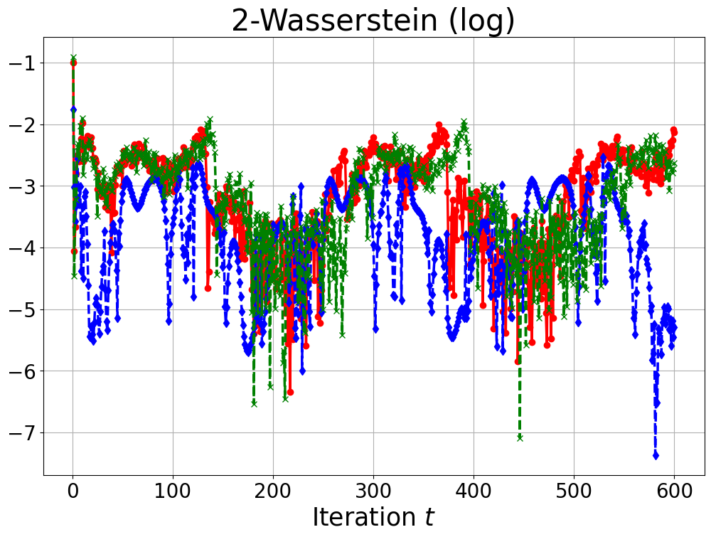
Our objective is to simulate the state trajectories of this dynamical system. Starting with an initial point , at iteration , we draw a posterior GP sampling from the conditional distribution , where denotes the set of the training data along with the current trajectory . In our implementation, we choose the model eq. 29 with step size , parameters , , , noise variance , and initial point . The training set was generated by evaluating eq. 29 at points , which are uniformly distributed in the interval , with corresponding currents chosen uniformly from . Variations in each step were simulated using independent Matérn 3/2 GPs with and inducing points approximation on the sparse grid . We generate 1000 samples at each iteration. Figure 7 presents the state trajectories of voltage and recovery variable versus the iteration step for each algorithm. The left plots in Figure 7 show that our proposed algorithm can accurately characterize the state trajectories of this dynamical system. Figure 8 illustrates the computational time required for each iteration and the 2-Wasserstein distance between the states derived from GP-based simulations and those obtained using the Euler–Maruyama method as described in eq. 28 at each iteration . These results demonstrate that our proposed algorithm not only reduces the computational time but also preserves accuracy that is comparable to the decoupled method.
5 Conclusion
In this work, we propose a scalable algorithm for GP sampling using inducing points on a sparse grid, which only requires a time complexity of for sampling points, a sparse grid of size and level . Additionally, we show that the convergence rate for GP sampling with a sparse grid is for a -dimensional sparse grid of size and a product Matérn kernel of smoothness . For the posterior samplings, we develop a two-level additive Schwarz preconditioner for the matrix over the sparse grid, which empirically shows rapid convergence. In the numerical study, we demonstrate that the proposed algorithm is not only efficient but also maintains accuracy comparable to other approximation methods.
Acknowledgments and Disclosure of Funding
This work is supported by NSF grants DMS-2312173 and CNS-2328395.
Appendix A Theorems
A.1 Rate of convergence
Theorem A.1.
Let for any . Let be a GP on with a Matérn kernel defined in eq. 6 with smoothness , and be an inducing points approximation of under the inducing points for some positive integer . Then for any , as , the order of magnitude of the approximation error is
Proof.
Note that and already live in the same probability space, that is . Therefore,
| (30) |
According to Theorem 4 in (Tuo and Wang, , 2020), has the order of magnitude and sub-Gaussian tails, which leads to the desired result. ∎
Lemma A.2.
[Adapted from Proposition 1 and Corollary 2 in (Rieger and Wendland, , 2017)] Let be a reproducing kernel of , where is the tensor product with and , is a reproducing kernel of Sobolev space of smoothness measured in -norm. Suppose we are given the sparse grid defined in eq. 10 over with points and an unknown function . Let be the solution to the norm-minimal interpolant on the sparse grid as follows:
| (31) |
Then, we have
| (32) |
where is a constant.
Proof.
See proofs of Proposition 1 and Corollary 2 in (Rieger and Wendland, , 2017). ∎
Theorem A.3.
Let for any , is the dimension of the space . Let be a GP on with a product Matérn kernel defined in eq. 5 with variance and base kernel of smoothness , and let be an inducing points approximation of under the inducing points on a sparse grid defined in eq. 10. We denote the cardinality of the sparse grid by . Then, as , the order of magnitude of the approximation error is
Proof.
If in Lemma A.2 is a Matérn kernel in one dimension, we can infer that by Lemma 15 in (Tuo and Wang, , 2020), which states that the reproducing kernel Hilbert space (RKHS) is a Sobolev space with equivalent norms. We denote RKHS associated with product Matérn kernel by and its norm by .
Let be the interpolation of the function with respect to the approximation . Clearly, . Proposition 2 in (Rieger and Wendland, , 2017) asserts that where is norm-minimal interpolant defined in Lemma A.2. Therefore, for any , we have
| (33) |
Additionally, Lemma 15 in (Tuo and Wang, , 2020) implies that
| (34) |
Note that and already live in the same probability space, that is . Therefore, by combining with eq. 33 and eq. 34, we can obtain the following results:
| (35) |
Thus, the order of the magnitude of the inducing points approximation on the sparse grid error is . ∎
A.2 Smolyak algorithm for GP sampling
Theorem A.4.
Let be a kernel function on , and a sparse grid design with level and dimension defined in eq. 10. where , , , . Let be a GP, then sampling from on a sparse grid can be done via the following formula:
| (36) |
| (37) |
where , is the Cholesky decomposition of , is standard multivariate normal distributed, is the size of the full grid design associated with , is a Dirac measure on the set .
Proof.
We know that sampling from can be done via Cholesky decomposition, i.e., by computing where is multivariate normal distributed on the sparse grid of size . Note that can be regarded as a function evaluated on such that . According to eq. 12, we can obtain the following equation by applying Smolyak’s algorithm to ,
| (38) | ||||
where and are defined in eq. 37. Note that is defined on , so the tensor product operation on is actually evaluating on the corresponding points, which is equivalent to applying Dirac delta measure defined on set to . ∎
Appendix B Plots


References
- Ackley, (2012) Ackley, D. (2012). A connectionist machine for genetic hillclimbing, volume 28. Springer Science & Business Media.
- Al Daas and Grigori, (2019) Al Daas, H. and Grigori, L. (2019). A class of efficient locally constructed preconditioners based on coarse spaces. SIAM Journal on Matrix Analysis and Applications, 40(1):66–91.
- Al Daas et al., (2023) Al Daas, H., Jolivet, P., and Rees, T. (2023). Efficient Algebraic Two-Level Schwarz Preconditioner for Sparse Matrices. SIAM Journal on Scientific Computing, 45(3):A1199–A1213.
- Banerjee et al., (2008) Banerjee, S., Gelfand, A. E., Finley, A. O., and Sang, H. (2008). Gaussian predictive process models for large spatial data sets. Journal of the Royal Statistical Society Series B: Statistical Methodology, 70(4):825–848.
- Bishop et al., (1995) Bishop, C. M. et al. (1995). Neural networks for pattern recognition. Oxford university press.
- Cai and Sarkis, (1999) Cai, X.-C. and Sarkis, M. (1999). A restricted additive Schwarz preconditioner for general sparse linear systems. Siam journal on scientific computing, 21(2):792–797.
- Chen et al., (2022) Chen, H., Ding, L., and Tuo, R. (2022). Kernel packet: An Exact and Scalable Algorithm for Gaussian Process Regression with Matérn Correlations. Journal of Machine Learning Research, 23(127):1–32.
- Chen and Tuo, (2022) Chen, H. and Tuo, R. (2022). A Scalable and Exact Gaussian Process Sampler via Kernel Packets.
- Cole et al., (2021) Cole, D. A., Christianson, R. B., and Gramacy, R. B. (2021). Locally induced Gaussian processes for large-scale simulation experiments. Statistics and Computing, 31:1–21.
- Constantinou et al., (2017) Constantinou, P., Kokoszka, P., and Reimherr, M. (2017). Testing separability of space-time functional processes. Biometrika, 104(2):425–437.
- Cressie, (2015) Cressie, N. (2015). Statistics for spatial data. John Wiley & Sons.
- Curriero, (2006) Curriero, F. C. (2006). On the use of non-Euclidean distance measures in geostatistics. Mathematical Geology, 38:907–926.
- Cutajar et al., (2016) Cutajar, K., Osborne, M., Cunningham, J., and Filippone, M. (2016). Preconditioning kernel matrices. In International conference on machine learning, pages 2529–2538. PMLR.
- Demmel, (1997) Demmel, J. W. (1997). Applied numerical linear algebra. SIAM.
- Diggle et al., (2003) Diggle, P. J., Ribeiro, P. J., and Christensen, O. F. (2003). An introduction to model-based geostatistics. Spatial statistics and computational methods, pages 43–86.
- Ding et al., (2021) Ding, L., Tuo, R., and Shahrampour, S. (2021). A sparse expansion for deep gaussian processes. arXiv preprint arXiv:2112.05888.
- Dolean et al., (2015) Dolean, V., Jolivet, P., and Nataf, F. (2015). An introduction to domain decomposition methods: algorithms, theory, and parallel implementation. SIAM.
- Dowson and Landau, (1982) Dowson, D. and Landau, B. (1982). The Fréchet distance between multivariate normal distributions. Journal of multivariate analysis, 12(3):450–455.
- Dryja and Widlund, (1994) Dryja, M. and Widlund, O. B. (1994). Domain decomposition algorithms with small overlap. SIAM Journal on Scientific Computing, 15(3):604–620.
- Engel et al., (2005) Engel, Y., Mannor, S., and Meir, R. (2005). Reinforcement learning with Gaussian processes. In Proceedings of the 22nd international conference on Machine learning, pages 201–208.
- FitzHugh, (1961) FitzHugh, R. (1961). Impulses and physiological states in theoretical models of nerve membrane. Biophysical journal, 1(6):445–466.
- (22) Frazier, P. I. (2018a). A tutorial on Bayesian optimization. arXiv preprint arXiv:1807.02811.
- (23) Frazier, P. I. (2018b). Bayesian optimization. In Recent advances in optimization and modeling of contemporary problems, pages 255–278. Informs.
- Garcke, (2013) Garcke, J. (2013). Sparse grids in a nutshell. In Sparse grids and applications, pages 57–80. Springer.
- Gardner et al., (2018) Gardner, J., Pleiss, G., Weinberger, K. Q., Bindel, D., and Wilson, A. G. (2018). Gpytorch: Blackbox matrix-matrix gaussian process inference with gpu acceleration. Advances in neural information processing systems, 31.
- Gelbrich, (1990) Gelbrich, M. (1990). On a formula for the L2 Wasserstein metric between measures on Euclidean and Hilbert spaces. Mathematische Nachrichten, 147(1):185–203.
- Genton, (2001) Genton, M. G. (2001). Classes of kernels for machine learning: a statistics perspective. Journal of machine learning research, 2(Dec):299–312.
- Genton, (2007) Genton, M. G. (2007). Separable approximations of space-time covariance matrices. Environmetrics: The official journal of the International Environmetrics Society, 18(7):681–695.
- Girard et al., (2002) Girard, A., Rasmussen, C., Candela, J. Q., and Murray-Smith, R. (2002). Gaussian process priors with uncertain inputs application to multiple-step ahead time series forecasting. Advances in neural information processing systems, 15.
- Gneiting et al., (2006) Gneiting, T., Genton, M. G., and Guttorp, P. (2006). Geostatistical space-time models, stationarity, separability, and full symmetry. Monographs On Statistics and Applied Probability, 107:151.
- Golub and Van Loan, (2013) Golub, G. H. and Van Loan, C. F. (2013). Matrix Computations. JHU press.
- Gramacy and Apley, (2015) Gramacy, R. B. and Apley, D. W. (2015). Local Gaussian process approximation for large computer experiments. Journal of Computational and Graphical Statistics, 24(2):561–578.
- Grande et al., (2014) Grande, R., Walsh, T., and How, J. (2014). Sample efficient reinforcement learning with Gaussian processes. In International Conference on Machine Learning, pages 1332–1340. PMLR.
- Griewank, (1981) Griewank, A. O. (1981). Generalized descent for global optimization. Journal of optimization theory and applications, 34(1):11–39.
- Grigorievskiy et al., (2017) Grigorievskiy, A., Lawrence, N., and Särkkä, S. (2017). Parallelizable sparse inverse formulation Gaussian processes (SpInGP). In 2017 IEEE 27th International Workshop on Machine Learning for Signal Processing (MLSP), pages 1–6. IEEE.
- Hartikainen and Särkkä, (2010) Hartikainen, J. and Särkkä, S. (2010). Kalman filtering and smoothing solutions to temporal Gaussian process regression models. In 2010 IEEE international workshop on machine learning for signal processing, pages 379–384. IEEE.
- Henderson et al., (1983) Henderson, H. V., Pukelsheim, F., and Searle, S. R. (1983). On the history of the Kronecker product. Linear and Multilinear Algebra, 14(2):113–120.
- Hensman et al., (2018) Hensman, J., Durrande, N., and Solin, A. (2018). Variational Fourier features for Gaussian processes. Journal of Machine Learning Research, 18(151):1–52.
- Hensman et al., (2013) Hensman, J., Fusi, N., and Lawrence, N. D. (2013). Gaussian processes for big data. arXiv preprint arXiv:1309.6835.
- Hensman et al., (2015) Hensman, J., Matthews, A., and Ghahramani, Z. (2015). Scalable variational Gaussian process classification. In Artificial Intelligence and Statistics, pages 351–360. PMLR.
- Hestenes et al., (1952) Hestenes, M. R., Stiefel, E., et al. (1952). Methods of conjugate gradients for solving linear systems. Journal of research of the National Bureau of Standards, 49(6):409–436.
- Journel and Huijbregts, (1976) Journel, A. G. and Huijbregts, C. J. (1976). Mining geostatistics.
- Katzfuss and Guinness, (2021) Katzfuss, M. and Guinness, J. (2021). A general framework for Vecchia approximations of Gaussian processes. Statistical Science, 36(1):124–141.
- Katzfuss et al., (2022) Katzfuss, M., Guinness, J., and Lawrence, E. (2022). Scaled Vecchia approximation for fast computer-model emulation. SIAM/ASA Journal on Uncertainty Quantification, 10(2):537–554.
- Kennedy and O’Hagan, (2001) Kennedy, M. C. and O’Hagan, A. (2001). Bayesian calibration of computer models. Journal of the Royal Statistical Society: Series B (Statistical Methodology), 63(3):425–464.
- Kolda, (2006) Kolda, T. G. (2006). Multilinear operators for higher-order decompositions. Technical report, Sandia National Laboratories (SNL), Albuquerque, NM, and Livermore, CA ….
- Kuss and Rasmussen, (2003) Kuss, M. and Rasmussen, C. (2003). Gaussian processes in reinforcement learning. Advances in neural information processing systems, 16.
- Kuss et al., (2005) Kuss, M., Rasmussen, C. E., and Herbrich, R. (2005). Assessing Approximate Inference for Binary Gaussian Process Classification. Journal of machine learning research, 6(10).
- Lin et al., (2023) Lin, J. A., Antorán, J., Padhy, S., Janz, D., Hernández-Lobato, J. M., and Terenin, A. (2023). Sampling from Gaussian Process Posteriors using Stochastic Gradient Descent. arXiv preprint arXiv:2306.11589.
- MacKay et al., (2003) MacKay, D. J., Mac Kay, D. J., et al. (2003). Information theory, inference and learning algorithms. Cambridge university press.
- Maddox et al., (2021) Maddox, W. J., Balandat, M., Wilson, A. G., and Bakshy, E. (2021). Bayesian optimization with high-dimensional outputs. Advances in Neural Information Processing Systems, 34:19274–19287.
- Mallasto and Feragen, (2017) Mallasto, A. and Feragen, A. (2017). Learning from uncertain curves: The 2-Wasserstein metric for Gaussian processes. Advances in Neural Information Processing Systems, 30.
- Maruyama, (1955) Maruyama, G. (1955). Continuous Markov processes and stochastic equations. Rend. Circ. Mat. Palermo, 4:48–90.
- Marzouk and Najm, (2009) Marzouk, Y. M. and Najm, H. N. (2009). Dimensionality reduction and polynomial chaos acceleration of Bayesian inference in inverse problems. Journal of Computational Physics, 228(6):1862–1902.
- Murray-Smith and Pearlmutter, (2004) Murray-Smith, R. and Pearlmutter, B. A. (2004). Transformations of Gaussian process priors. In International Workshop on Deterministic and Statistical Methods in Machine Learning, pages 110–123. Springer.
- Nagumo et al., (1962) Nagumo, J., Arimoto, S., and Yoshizawa, S. (1962). An active pulse transmission line simulating nerve axon. Proceedings of the IRE, 50(10):2061–2070.
- Neal, (2012) Neal, R. M. (2012). Bayesian learning for neural networks, volume 118. Springer Science & Business Media.
- Nguyen et al., (2021) Nguyen, V., Deisenroth, M. P., and Osborne, M. A. (2021). Gaussian Process Sampling and Optimization with Approximate Upper and Lower Bounds. arXiv preprint arXiv:2110.12087.
- Nickisch and Rasmussen, (2008) Nickisch, H. and Rasmussen, C. E. (2008). Approximations for binary Gaussian process classification. Journal of Machine Learning Research, 9(Oct):2035–2078.
- Nickisch et al., (2018) Nickisch, H., Solin, A., and Grigorevskiy, A. (2018). State space Gaussian processes with non-Gaussian likelihood. In International Conference on Machine Learning, pages 3789–3798. PMLR.
- Nychka et al., (2015) Nychka, D., Bandyopadhyay, S., Hammerling, D., Lindgren, F., and Sain, S. (2015). A multiresolution Gaussian process model for the analysis of large spatial datasets. Journal of Computational and Graphical Statistics, 24(2):579–599.
- O’Hagan, (1978) O’Hagan, A. (1978). Curve fitting and optimal design for prediction. Journal of the Royal Statistical Society: Series B (Methodological), 40(1):1–24.
- Okhrin et al., (2020) Okhrin, Y., Schmid, W., and Semeniuk, I. (2020). New approaches for monitoring image data. IEEE Transactions on Image Processing, 30:921–933.
- Pardo-Iguzquiza and Chica-Olmo, (2008) Pardo-Iguzquiza, E. and Chica-Olmo, M. (2008). Geostatistics with the Matern semivariogram model: A library of computer programs for inference, kriging and simulation. Computers & Geosciences, 34(9):1073–1079.
- Plumlee, (2014) Plumlee, M. (2014). Fast prediction of deterministic functions using sparse grid experimental designs. Journal of the American Statistical Association, 109(508):1581–1591.
- Plumlee, (2017) Plumlee, M. (2017). Bayesian calibration of inexact computer models. Journal of the American Statistical Association, 112(519):1274–1285.
- Quinonero-Candela and Rasmussen, (2005) Quinonero-Candela, J. and Rasmussen, C. E. (2005). A unifying view of sparse approximate Gaussian process regression. The Journal of Machine Learning Research, 6:1939–1959.
- Rahimi and Recht, (2007) Rahimi, A. and Recht, B. (2007). Random features for large-scale kernel machines. Advances in neural information processing systems, 20.
- Rasmussen, (2003) Rasmussen, C. E. (2003). Gaussian processes in machine learning. In Summer school on machine learning, pages 63–71. Springer.
- Rieger and Wendland, (2017) Rieger, C. and Wendland, H. (2017). Sampling inequalities for sparse grids. Numerische Mathematik, 136:439–466.
- Roberts et al., (2013) Roberts, S., Osborne, M., Ebden, M., Reece, S., Gibson, N., and Aigrain, S. (2013). Gaussian processes for time-series modelling. Philosophical Transactions of the Royal Society A: Mathematical, Physical and Engineering Sciences, 371(1984):20110550.
- Saad, (2003) Saad, Y. (2003). Iterative methods for sparse linear systems. SIAM.
- Saatçi, (2012) Saatçi, Y. (2012). Scalable inference for structured Gaussian process models. PhD thesis, Citeseer.
- Santner et al., (2003) Santner, T. J., Williams, B. J., Notz, W. I., and Williams, B. J. (2003). The design and analysis of computer experiments, volume 1. Springer.
- Shewchuk et al., (1994) Shewchuk, J. R. et al. (1994). An introduction to the conjugate gradient method without the agonizing pain.
- Silverman, (1985) Silverman, B. W. (1985). Some aspects of the spline smoothing approach to non-parametric regression curve fitting. Journal of the Royal Statistical Society: Series B (Methodological), 47(1):1–21.
- Smolyak, (1963) Smolyak, S. A. (1963). Quadrature and interpolation formulas for tensor products of certain classes of functions. In Doklady Akademii Nauk, volume 148, pages 1042–1045. Russian Academy of Sciences.
- Snoek et al., (2012) Snoek, J., Larochelle, H., and Adams, R. P. (2012). Practical bayesian optimization of machine learning algorithms. Advances in neural information processing systems, 25.
- Spillane et al., (2014) Spillane, N., Dolean, V., Hauret, P., Nataf, F., Pechstein, C., and Scheichl, R. (2014). Abstract robust coarse spaces for systems of PDEs via generalized eigenproblems in the overlaps. Numerische Mathematik, 126:741–770.
- Srinivas et al., (2009) Srinivas, N., Krause, A., Kakade, S. M., and Seeger, M. (2009). Gaussian process optimization in the bandit setting: No regret and experimental design. arXiv preprint arXiv:0912.3995.
- Stanton et al., (2021) Stanton, S., Maddox, W., Delbridge, I., and Wilson, A. G. (2021). Kernel interpolation for scalable online Gaussian processes. In International Conference on Artificial Intelligence and Statistics, pages 3133–3141. PMLR.
- Stein, (1999) Stein, M. L. (1999). Interpolation of spatial data: some theory for kriging. Springer Science & Business Media.
- Teckentrup, (2020) Teckentrup, A. L. (2020). Convergence of Gaussian process regression with estimated hyper-parameters and applications in Bayesian inverse problems. SIAM/ASA Journal on Uncertainty Quantification, 8(4):1310–1337.
- Thompson, (1933) Thompson, W. R. (1933). On the likelihood that one unknown probability exceeds another in view of the evidence of two samples. Biometrika, 25(3-4):285–294.
- Titsias, (2009) Titsias, M. (2009). Variational learning of inducing variables in sparse Gaussian processes. In Artificial intelligence and statistics, pages 567–574. PMLR.
- Toselli and Widlund, (2004) Toselli, A. and Widlund, O. (2004). Domain decomposition methods-algorithms and theory, volume 34. Springer Science & Business Media.
- Trefethen and Bau III, (1997) Trefethen, L. N. and Bau III, D. (1997). Numerical linear algebra, vol. 50.
- Tuo and Wang, (2020) Tuo, R. and Wang, W. (2020). Kriging prediction with isotropic Matérn correlations: Robustness and experimental designs. The Journal of Machine Learning Research, 21(1):7604–7641.
- Tuo and Wu, (2015) Tuo, R. and Wu, C. J. (2015). Efficient calibration for imperfect computer models. The Annals of Statistics, 43(6):2331 – 2352.
- Ullrich, (2008) Ullrich, T. (2008). Smolyak’s algorithm, sampling on sparse grids and Sobolev spaces of dominating mixed smoothness. East Journal of Approximations, 14(1):1.
- Van der Vorst, (2003) Van der Vorst, H. A. (2003). Iterative Krylov methods for large linear systems. Number 13. Cambridge University Press.
- Wang et al., (2019) Wang, K., Pleiss, G., Gardner, J., Tyree, S., Weinberger, K. Q., and Wilson, A. G. (2019). Exact Gaussian processes on a million data points. Advances in neural information processing systems, 32.
- Wang et al., (2020) Wang, W., Tuo, R., and Jeff Wu, C. (2020). On prediction properties of kriging: Uniform error bounds and robustness. Journal of the American Statistical Association, 115(530):920–930.
- (94) Wenger, J., Pleiss, G., Hennig, P., Cunningham, J., and Gardner, J. (2022a). Preconditioning for scalable Gaussian process hyperparameter optimization. In International Conference on Machine Learning, pages 23751–23780. PMLR.
- (95) Wenger, J., Pleiss, G., Pförtner, M., Hennig, P., and Cunningham, J. P. (2022b). Posterior and computational uncertainty in gaussian processes. Advances in Neural Information Processing Systems, 35:10876–10890.
- Williams and Seeger, (2000) Williams, C. and Seeger, M. (2000). Using the Nyström method to speed up kernel machines. Advances in neural information processing systems, 13.
- Williams and Rasmussen, (2006) Williams, C. K. and Rasmussen, C. E. (2006). Gaussian processes for machine learning, volume 2. MIT press Cambridge, MA.
- Wilson and Nickisch, (2015) Wilson, A. and Nickisch, H. (2015). Kernel interpolation for scalable structured Gaussian processes (KISS-GP). In International conference on machine learning, pages 1775–1784. PMLR.
- Wilson et al., (2020) Wilson, J., Borovitskiy, V., Terenin, A., Mostowsky, P., and Deisenroth, M. (2020). Efficiently sampling functions from Gaussian process posteriors. In International Conference on Machine Learning, pages 10292–10302. PMLR.
- Wilson et al., (2021) Wilson, J. T., Borovitskiy, V., Terenin, A., Mostowsky, P., and Deisenroth, M. P. (2021). Pathwise Conditioning of Gaussian Processes. J. Mach. Learn. Res., 22:105–1.
- Xie and Xu, (2021) Xie, F. and Xu, Y. (2021). Bayesian projected calibration of computer models. Journal of the American Statistical Association, 116(536):1965–1982.
- Yadav et al., (2022) Yadav, M., Sheldon, D. R., and Musco, C. (2022). Kernel Interpolation with Sparse Grids. Advances in Neural Information Processing Systems, 35:22883–22894.
- Zafari et al., (2020) Zafari, S., Murashkina, M., Eerola, T., Sampo, J., Kälviäinen, H., and Haario, H. (2020). Resolving overlapping convex objects in silhouette images by concavity analysis and Gaussian process. Journal of Visual Communication and Image Representation, 73:102962.