Gaussian Processes for Time Series with Lead-Lag Effects with application to biology data
Abstract
Investigating the relationship, particularly the lead-lag effect, between time series is a common question across various disciplines, especially when uncovering biological process. However, analyzing time series presents several challenges. Firstly, due to technical reasons, the time points at which observations are made are not at uniform intervals. Secondly, some lead-lag effects are transient, necessitating time-lag estimation based on a limited number of time points. Thirdly, external factors also impact these time series, requiring a similarity metric to assess the lead-lag relationship. To counter these issues, we introduce a model grounded in the Gaussian process, affording the flexibility to estimate lead-lag effects for irregular time series. In addition, our method outputs dissimilarity scores, thereby broadening its applications to include tasks such as ranking or clustering multiple pair-wise time series when considering their strength of lead-lag effects with external factors. Crucially, we offer a series of theoretical proofs to substantiate the validity of our proposed kernels and the identifiability of kernel parameters. Our model demonstrates advances in various simulations and real-world applications, particularly in the study of dynamic chromatin interactions, compared to other leading methods.
1 Introduction
The lead-lag effect, a widespread phenomenon where changes in one time series (the leading series) influence another time series (the influenced follower series) after a certain delay. This phenomenon is prevalent in a variety of fields, such as climate science (De Luca and Pizzolante, 2021), healthcare (Runge et al., 2019; Zhu and Gallego, 2021; Feng et al., 2021), economics (Wang et al., 2017; Skoura, 2019), and finance (Hoffmann et al., 2013; Bacry et al., 2013; Da Fonseca and Zaatour, 2017; Ito and Sakemoto, 2020). For example, Harzallah and Sadourny (1997) explores the lead-lag relationship between the Indian summer monsoon and various climate variables, such as sea surface temperature, snow cover, and geopotential height. However, this dynamic, rooted in causal regulatory relationships, is notably observed in biological processes, which serves as the primary inspiration for the proposed method. The lead-lag effect manifests itself in various processes, including development (Gerstein et al., 2010; Ding and Bar-Joseph, 2020; Strober et al., 2019), disease-associated genetic variation (Krijger and De Laat, 2016), and responses to various interventions and treatments (Faryabi et al., 2008; Lu et al., 2021).
To provide a clearer context for this concept, we consider temporal-omics datasets, particularly those used in the identification of potential enhancer-promoter pairs in various biological processes (Whalen et al., 2016; Fulco et al., 2019; Schoenfelder and Fraser, 2019; Moore et al., 2020). Enhancers are short cis-regulatory DNA sequences that are distal to the genes they regulate, as opposed to the promoter sequence that is adjacent to a particular gene. Since enhancers and promoters coordinate to generate time- and context-specific gene expression programs, that is, the amount of RNA produced at what time, we hypothesize that the dynamic patterns of enhancer regulation are typically followed by corresponding gene program patterns, albeit with a certain time lag. Approximately a million candidate human enhancers have been identified (Moore et al., 2020), though the intricate dynamics of how and which enhancers interact with promoters in specific processes is still an area of active and ongoing research.
Addressing this challenge, our study focuses on the multi-omics time series data presented by Reed et al. (2022). This dataset includes measurements of enhancer activity, and promoter transcription, and 3D chromatin structure at seven time points, from 0 to 6 hours (a later time point is excluded from this analysis). These data reveal complex dynamic patterns, as depicted in Figure 1. Our goal is to identify functional human enhancer-promoter pairs from over 20,000 candidate pairs, estimate the time lag, and quantify the extent of the lead-lag effect between enhancer activity and gene expression over time. The biological motivation for this goal is to uncover a relationship in genomics time series for a subset of enhancer-gene pairs, in particular those in which the enhancer state changes after cell activation and causes a subsequent change in expression of a target gene. Measuring the lag between enhancer activity and gene expression over time for these candidate enhancer-promoter pairs helps in understanding the sequence of regulatory events set off by activation, and how the time scale of gene regulation may vary across the genome.

In the context of our motivating application involving multi-omics time series data, and similar scenarios across various fields, there are key challenges that need careful consideration. Firstly, a common issue is the scarcity of time-point observations. This limitation is compounded by the irregular intervals between successive measurements, often due to the high cost of experimental design or sensor failures. Additionally, in cases where there is an abundance of time-point data, the focus may shift to pinpointing local time delays within smaller segments of the time series. These factors underscore the importance of accurately quantifying the uncertainty associated with the extent of the lead-lag relationship, particularly when dealing with limited temporal datasets.
Existing methods for aligning time-lagged time series to explore the magnitude of lead-lag effects are numerous and varied. This exploration can extend to tasks such as ranking leaders or followers among multiple time series (Wu et al., 2010) and performing network clustering of time series based on the pairwise lead-lag relationships (Bennett et al., 2022). For example, Wu et al. (2010) ranks the leaders of the streams to the sea surface temperature. Widely used models such as time-lagged cross-correlation (TLCC, Shen (2015)) by comparing the cross-correlation coefficients, dynamic time warping (DTW, Berndt and Clifford (1994)), and its differentiable approximation, soft-DTW (Cuturi and Blondel, 2017), and soft-DTW divergence (Blondel et al., 2021) have proven useful by comparing distance loss among multiple pairwise time series after alignment (De Luca and Pizzolante, 2021). TLCC, for instance, operates by sliding one signal over another and identifying the shift position with the highest correlation. However, these methods often require the same time intervals for each time series, which makes them less effective for irregular time series, potentially leading to distortions of the true underlying relationships.
Beyond quantifying the lead-lag effect between pairwise time series, there is often a desire to estimate time lag considering the irregularities in time series data, one approach is to first impute values at regular time points, then apply methods like TLCC to calculate the time lag. Common techniques for this separate modeling of each time series include using splines (Rehfeld et al., 2011) or separate Gaussian processes (SGP, Li et al. (2021)). However, such methods do not leverage shared information across time series, potentially leading to sub-optimal results. Hierarchical GP models such as Magma (Leroy et al., 2022, 2023) integrate shared information across multiple time series but are primarily designed for prediction and clustering individual time series. This is in contrast to our primary objective, which is to cluster pairwise time series by a measure of similarity. More direct approaches for irregular time series include the use of the negative and positive lead-lag estimator (NAPLES, Ito and Nakagawa (2020)) and Lead-Lag method (Hoffmann et al., 2013), which utilize the Hayashi–Yoshida covariance estimator to estimate a fixed time-lag. Alternatively, multi-task GPs through latent variable models introduce additional variables to account for temporal discrepancies such as GPLVM (Dürichen et al., 2014), which may limit flexibility due to the presumed independence between tasks and temporal sequences (also known as separable kernels). Moreover, more complex misalignment techniques (Kazlauskaite et al., 2019; Mikheeva et al., 2022) might not perform well with limited time observations for biology data where simpler linear mismatch assumptions suffice, and they can face operational challenges like Cholesky decomposition failures. Table 1 compares the aforementioned methods, highlighting their suitability for limited or irregular time points, their ability to quantify the magnitude of lead-lag effects, and estimate time lags:
| Quantify the magnitude of lead-lag effect | Estimate time lag | |||||||||||
|---|---|---|---|---|---|---|---|---|---|---|---|---|
| Model |
|
|
|
|
||||||||
| TLCC | X | X | ||||||||||
| DTW | X | X | ||||||||||
| Lead-Lag | X | X | ||||||||||
| SGP | X∗ | X∗ | X∗ | X∗ | ||||||||
| Splines | X∗ | X∗ | X∗ | X∗ | ||||||||
| GPLVM | X∗ | X∗ | ||||||||||
| MAGMA | X∗ | X∗ | ||||||||||
| GPlag | X | X | X | X | ||||||||
Note: X∗ means yes if followed by TLCC or DTW.
In response to these challenges and limitations of existing methods, we propose the Gaussian Process for lead-lag time series (GPlag) model. GPlag introduces a novel class of GP kernels for time series with lead-lag effects, featuring interpretable parameters that estimate both the time lag and the degree of lead-lag effects. These parameters are crucial for tasks such as identifying associated factors, ranking or clustering time series based on lead-lag relationships. Our model also provides theoretical justification for the identifiability and interpretability of these key parameters, and integrates a Bayesian framework for greater flexibility in handling time series with constraints like limited observations or irregular time gaps.
2 Methods
2.1 Gaussian Process
Gaussian processes are widely used for modelling dependency structures, such as spatial statistics and time series modelling. In generic terms, a Gaussian process models a random function where any finite collection of realizations (i.e., observations) follow a multivariate normal (MVN) distribution.
Definition 1.
follows a Gaussian process with mean function and covariance function , denoted by , if for any , , where and .
Covariance functions, also known as kernels, are widely studied when , such as the radial basis function (RBF, also known as the squared exponential kernel), the exponential kernel, and the Matérn kernel (Stein, 1999).
2.2 Pairwise Time Series Gaussian Process Model
For the sake of clarity, we initiate pairwise time series models, and the extension to multiple time series is delayed to Section 2.5. Given a pair of time series , where , we model as a multi-output Gaussian process: . Here, and represents the measurement error. The mean function is defined as , and is a cross-covariance kernel, with representing the space of all 2 by 2 positive definite matrices. is often assumed to be zero, which can be achieved by a vertical shift (Gelfand et al., 2010), so we assume in the remaining sections.
The cross-covariance kernel is a crucial component of the model, expected to incorporate both the relationship between and , and the time lag. Constructing valid cross-covariance kernels is a recognized challenge (Gneiting et al., 2010; Apanasovich and Genton, 2010; Genton and Kleiber, 2015), even more so when kernels must have certain identifiable and interpretable parameters in biological applications.
We address this by transforming the problem to its “dual” state, converting the multi-output GP into a single-output GP via , where is a single-output GP, , and . Here, is a covariance kernel of a single-output GP, but the domain expands to instead of . Essentially, we transform a multi-output GP over into a single-output GP over , where is an index set of time series. This simplifies the problem by increasing the complexity of the domain.”
In this newly formed domain , a family of inseparable, semi-stationary kernel has been developed by (Li et al., 2021), i.e., for any . Consequently, can be reformulated as a function on as . However, for simplicity, we will denote both as in the subsequent sections. A rich family of semi-stationary kernels can be found in (Li et al., 2021). This family of kernels, although rich, was not specifically designed for time series with a time lag. To account for the time lag, the following theorem ensures that any existing semi-stationary kernel can induce a kernel with a parameter that measures the time lag, denoted by , which ensures that our proposed kernel, with the inclusion of this time lag parameter, remains a valid kernel within the GP framework.
Theorem 1.
Let be a semi-stationary kernel on , then the induced kernel defined as
| (1) |
is positive definite, and thus serves as a covariance kernel for a GP, where measures the time lag between two time series.
The following corollary provides some concrete candidates of kernels for GPlag:
Corollary 1.
If is a completely monotone function and is a non-negative function with a completely monotone derivative, then
is a valid kernel, where measures the spatial variance, measures the time lag.
The proof is given in Section A.1. Since the key idea in the above theorem and corollary is motivated by Gneiting (2002), we call the kernel family constructed from Corollary 1 the Gneiting family. In particular, Gneiting enumerates four candidates for and three for in Gneiting (2002). Exploring each amalgamation of and families allows for further tailoring by adjusting parameters intrinsic to the family, culminating in the desired kernel. Furthermore, more kernels can be constructed by combining kernels from Gneiting family and other simple kernels. Analogues of the RBF, exponential kernel, and Matérn kernel in Euclidean space are provided in the following definitions.
Definition 2.
The following covariance kernel is called the time lag radial basis function (LRBF):
| (2) |
Definition 3.
The following covariance kernel is called the time lag exponential kernel (LExp):
| (3) |
Definition 4.
The following covariance kernel is called the time lag Matérn kernel (LMat) with smoothness :
| (4) |
As an illustration, LRBF can be derived by setting and in Corollary 1; LExp is the product of a kernel in Gneiting family with , , and a simple kernel ; LMat is the product of a kernel in Gneiting family with , , and a simple kernel . Common choices for are , where the Bessel function admits a closed form, similar to the standard Matérn kernel, with the specific choice depending on the data. Additional candidate kernels are presented in the Appendix A Appendix A, along with a detailed explanation on how they are constructed.
2.3 Interpretation of parameters
The interpretability of kernel parameters is one of the major advantages of GP models. In the kernels defined above, , the spatial variance, controls the point-wise variance; , the lengthscale parameter, governs the temporal dependency; the smoothness parameter determines the smoothness of the sample path. In this paper, we assume to be given, which is a common assumption in GP literature (Rasmussen, 2004). More importantly, , is called the dissimilarity parameter, where a smaller signifies a lesser degree of dissimilarity, which corresponds to a stronger lead-lag effect. For two distinct time series , when , the covariance , indicating independence between time series, or no lead-lag effect at all. On the other hand, when , , implying that the two time series are the same up to a time lag, the strongest lead-lag effect. The interpretation of in GPlag parallels measures lead-lag effect in other classical methods like DTW and TLCC: in GPlag aligns with a loss of 0 in DTW and a correlation of 1 in TLCC to signify the strongest lead-lag effect. Similarly, in GPlag corresponds to a loss of infinity in DTW and a correlation of 0 in TLCC for the weakest effect. The time lag parameter measures the time lag between two time series. In the next subsection, we discuss the implementation of GPlag and the inference of these parameters, especially and . Further visualization of sample paths of above kernels with different combinations of parameters are provided in Figure S5-Figure S7. Theoretical support for the identifiability of and is provided in Section 3.
2.4 Implementation
In this section, we outline the algorithm to estimate the parameters proposed in previous model, given the observations . The most direct approach is to find the maximum likelihood estimator (MLE) given by:
| (5) |
where denotes the vector of observations, and is the covariance matrix specified in Equations 2, 3 and 4. Optimization methods such as L-BFGS-B (Byrd et al., 1995) and Adam (Kingma and Ba, 2014) are widely used. The L-BFGS-B algorithm allows for setting lower and upper bounds on the parameters, enhancing the stability of the numeric optimization. The parameters are constrained to be positive and can be set to a reasonable range depending on specific cases. For the initial values of , we suggest running a standard GP regression first and using the estimates as our initial values. For , we recommend taking the estimate from TLCC, and we recommend as the initialization. The illustration of MLE process is provided in Appendix A Algorithm 1.
The extension to Bayesian inference is straightforward: we can simply sample from the posterior , where is the joint prior distribution. We suggest using independent inverse Gamma priors for and a Gaussian prior for . The algorithm is depicted in Algorithm 3 in Section A.3 and has been implemented in Python using GPyTorch (Gardner et al., 2018) and the Pyro (Bingham et al., 2019) package. This implementation enables rapid, fully Bayesian inference and takes advantage of GPU acceleration.
2.5 Extension to multi-time series
The kernels introduced in Section 2.2 can be extended to accommodate any number of time series, denoted by . Following the same rationale, it suffices to define a kernel on where . The following theorem generalizes LRBF, LExp and LMat for any by aligning with the criteria for a distance metric, parameterized by under the constraints for any and :
Theorem 2.
The following covariance functions are extensions of LRBF, LExp and LMat:
The positive definite, symmetric, and triangle inequality constraints on ensures the positive definiteness of , while the constraint on is due to our treating the first time series as the baseline, meaning that the time lag is relative to the first time series. The inference is similar to the previous case, with the only difference being that the optimization method involved in MLE needs to consider these additional constraints. In other words, it is a constrained optimization problem. Nevertheless, it is not intractable, as all the constraints on are linear and can be accommodated by existing optimization methods, including L-BFGS-B and Adam, as illustrated in Appendix A Algorithm 2 with three time series.
3 Identifiability of GPlag Kernel Parameter
To support our interpretation to and in Section 2, we discuss the identifiability, i.e., different parameters lead to different models. Note that not all parameters of commonly used GP models are identifiable, which means that different parameter values can lead to the same model. For example, in the classical Matérn covariance function, the spatial variance and lengthscale parameter are not identifiable, meaning that it is not possible to distinguish between different values of these parameters based on the data alone (Stein, 1999; Zhang, 2004; Kaufman and Shaby, 2013; Li et al., 2023; Li, 2022). This can be a limitation of GP models and it is important to consider when interpreting the results. In the case of GPlag, if the key parameters and are not identifiable, i.e., the GPlag determined by is equivalent to the one determined by , then it is unconvincing to interpret and as times series dissimilarity and time lag. Without identifiability, and do not admit any clear interpretation and the results of the model would be hard to interpret.
In this section, we prove that the parameters and in GPlag model are identifiable, allowing them to be used to as measures of the lead lag effect between time series (measured by ) and the time lag (measured by ). Here, we assume all parameters are positive, finite, real numbers, and the domain is fixed (also known as infill domain). The fixed domain assumption is reasonable for multi-omics time series, as the dynamics of gene regulation in such experiments occur during a fixed window of time. Investigators will decide, based on available budget, the time points needed to capture the dynamics during, say activation, or differentiation. If allocated more budget, they will then fill in the gaps between existing observations, to have better resolution over the same time period. We begin by introducing the necessary definitions.
Definition 5.
Two Gaussian processes and are said to be equivalent, denoted by , if the corresponding Gaussian random measures are equivalent to each other. That is, two Gaussian random measures are absolutely continuous with respect to each other.
If , then can never be correctly distinguished from regardless how dense the observed time points are (Zhang, 2004). Focusing on a parametric family of covariance functions , if there exists such that , then any estimator of based on observations , denoted by , cannot be weakly consistent (Dudley, 1989).
Definition 6.
is said to be identifiable if .
As a result, it suffices to show the following necessary and sufficient conditions for two GPlags being equivalent, which suggests identifiable parameters for further interpretation:
Theorem 3.
Let and be two LMat kernels with parameters and and is assumed to be known, then
That is, the identifiable parameters, also known as the microergodic parameters, are . In particular, let , the microergodic parameters for LExp kernel are .
The proof is given in Appendix A.2. Although and in GPlag are not identifiable, the proposed interpretation of the model does not rely on these two parameters. Instead, the parameter is interpreted as a measure of dissimilarity between time series under a time lag represented by the parameter .
It is important to note that GPs are commonly used for prediction and regression tasks. For this purpose, even though some kernel parameters such as and are not identifiable in these models, the prediction performance remains asymptotically optimal when the kernel parameters are mis-specified (Kaufman and Shaby, 2013). This is because regression is a distinct problem from parameter inference in GPs.
It is also worth noting that the identifiability of kernel parameters in GPs depends on the dimension of the domain. For time series, the domain is a 1-dimensional interval in . However, our theorem holds for 2-dimensional and 3-dimensional domains. In dimensions greater than , it becomes a challenging problem and we treat it as a future work since our focus of this work is one-dimensional time series.
4 Simulation studies
The main focus of our experiments was to illustrate that GPlag could accurately estimate both the time lag and the extent of lead-lag effects. This capability aided in the ranking or clustering of multiple time series that existed in a lead-lag relationship with a target time series. We demonstrated the theoretical properties of GPlag using synthetic data, as these properties were best illustrated under a fully controlled environment. All code and additional implementation details were available in the Section B.1.
Baseline models 1) For estimating the time lag, we compared with Lead-Lag (Hoffmann et al., 2013). 2) By utilizing the GP framework, we were able to predict values for two time series at unobserved time points. Then we evaluated the prediction error against three baselines: natural cubic splines with five breakpoints, SGP and Magma. 3) To evaluate the effectiveness of the estimate of lead-lag effects, we employed four baseline methods: TLCC, DTW, soft-DTW, and soft-DTW divergence. TLCC and DTW could output aligned time series, allowing us to calculate correlation coefficients from the aligned data. On the other hand, soft-DTW and soft-DTW divergence measured the amount of warping needed to align two time series and provided a distance loss metric. We used both correlation coefficients and distance loss as measures of dissimilarity between the time series.
Parameter estimation and inference. To validate the identifiability of our model, we simulated a pair of time series from GPlag with three kernels in Equations 2, 3 and 4, with 100 replicates. We set the mean to zero for both series and specified parameters as for each kernel. For LMat, we set the smoothness parameter as . The number of measurements within each time series varied across and the time points were generated following and , where and represents noise.

Our results showed that the MLE of and were very close to their truth among all three kernels when . This was consistent with the theoretical analysis in Theorem 3 (Figure 2 A, B) that GPlag could accurately recover the true lead-lag effects. Compared to Lead-Lag, GPlag exhibited similar or smaller variance, specifically when the kernel was Matérn with . Additionally, we performed simulations with a varying number of time points and found that the variance of the MLEs of and decreased as the sample size increased, which empirically confirmed the consistency of the MLEs (Figure 2 C). Plots for other parameters of secondary interest, including , , and , are provided in Figure S1. We also performed simulations with different settings of , and found that the consistency of the MLEs for and was maintained across these different values of (See Figure S2 for more details).
Prediction. We assessed the accuracy of GPlag’s predictions by generating data from two different processes. In the first, we used the kernel LExp in Equation 3 with parameters , and . In the second, we generated pairwise time series from linear functions with non-Gaussian noise (t-distributed): and where . The noise term, , were drawn from a t-distribution with 5 degrees of freedom. We then randomly selected of the data as training data for model fitting and used the remaining as testing data for prediction in both settings. We applied the best linear unbiased prediction (BLUP, see Section B.1 for more details) and used the mean squared error (MSE) on the testing set as the metric to evaluate the prediction accuracy.
Among all methods, GPlag achieved the highest log-likelihood and smallest MSE (Figure 3 A-B, Figure S3). The advantage of GPlag over SGP and splines was that it modeled two time series together which allowed for sharing of information between time series through . When , it was equivalent to SGP. While a small estimated indicated that two time series were similar, and the covariance function then allowed for more information to be shared between them. Although Magma adopted a hierarchical GP to specifically model the mean function for irregular data, it did not consider time lag information across time series.
Clustering or ranking time series based on dissimilarity to target time series.
We evaluated the relationship between the magnitude of parameter and the degree of lead-lag effects (the level of synchrony with a designated target signal) to assess the effectiveness of GPlag. We simulated nine time series from the function for every pair of and , where and . Among them, the time series simulated from the function of was treated as the target time series, which was close to a linear function (Figure 3 C, ts1). Each time series had times points ranging from . Here, determined the degree of distortion, where a smaller (e.g. 0.001) corresponded to a curve close to the identity transformation, and a larger represented the cases with more upward/downward distortion. By comparing different columns in Figure 3 C, we could see that the degree of dissimilarity between the target time series and other time series was controlled by , whereas controlled the time lag along the -axis.

Nine pairs of time series were fitted by GPlag with the LExp kernel. We observed that three pairs of time series in each column with the same were grouped together (Figure 3 D), and increased as increased. This implied that GPlag could accurately rank the degree of lead-lag effects among multiple pairs of time series based on the parameter , through precise estimation of the time lag parameter . A larger estimate of indicated a stronger dissimilarity between pairs of time series. To further quantify the clustering performance of lead-lag effects among the nine pairs of time series, we used the Adjusted Rand Index (ARI, Hubert and Arabie (1985)) and Normalized Mutual Information (NMI, Strehl and Ghosh (2002)) as evaluation metrics. To define a cluster from the pairwise dissimilarity parameter (correlation coefficients for TLCC and distance loss for DTWs), we used K-means (Shannon, 1948) with 3 clusters. As the focus of this work was on determining pairwise dissimilarity rather than the clustering algorithm, we opted for a simple clustering method. GPlag achieved the highest ARI and NMI in clustering the lead-lag effects among 9 pairwise time series (Table 1, column 2-3). We also tested GPlag using the LRBF and LMat kernels, and found that ARI and NMI scores remained at 1, consistent with the LExp results. The inferred values are shown in Figure S4, further indicating that the results are not sensitive to the choice of kernel.
| Synthetic data clustering | Dynamic Chromatin Interactions | |||||||
|---|---|---|---|---|---|---|---|---|
| Model | ARI | NMI |
|
|
||||
| TLCC | 0.35 | 0.58 | 0.051 | 0.13 | ||||
| DTW | 0.4 | 0.55 | 0.292 | 1 | ||||
| soft-DTW | 0.27 | 0.49 | 0.957 | 0.57 | ||||
| soft-DTW divergence | 0.07 | 0.39 | 0.907 | 0.90 | ||||
| GPlag | 1.00 | 1.00 | 0.019 | 0.05 | ||||
Note: Since the above algorithms are deterministic, the standard deviation is not reported.
Extension to three time series. To demonstrate the applicability of GPlag to more than two time series, we conducted simulation studies using three time series generated from the LExp kernel. In this scenario, all constraints were linear, allowing us to utilize optimizers that support linear constraints. Similar to the pairwise simulation setting, we set the mean to zero for all series, and the time points were generated according to the equations and , where and represented noise. The specified parameter values were . The maximum likelihood estimate (MLE) of the parameters closely approximated the true values (represented by the red dashed line), providing further validation of the theoretical properties. Additionally, the proposed method achieved the lowest mean squared error (MSE) in this particular setup (see Figure 4).

5 Genomics application: Dynamic chromatin interactions
In this section, we applied GPlag to a time-resolved multi-omics dataset involving enhancers and genes in human cells activated by interferon gamma from a resting state (Reed et al., 2022). Originally, the dataset comprised over 20,000 pairs. Each pair consisted of one time series for each enhancer and likewise one time series for each gene, at seven irregularly-spaced time points (0, 0.5, 1, 1.5, 2, 4, and 6 hours after a perturbation). The time series captured gene expression measurements for genes and histone tail acetylation measurements (H3K27ac), a measure of activity for the enhancers, both approximately variance stabilized. It is widely believed that the alterations in acetylation occur prior to the changes in expression of the regulated genes (Reed et al., 2022). We focused only on pairs that became functional after stimulation, by applying a filter on the total range of stabilized values across the timescale, yielding 4,776 dynamic pairs of enhancer-gene time series. Subsequently, the objective of our analysis, after estimating the model parameters of GPlag for these 4,776 pairs, was to identify the subset of all possible enhancer-gene pairs that represent functional enhancer-gene pairs, i.e. the enhancer responds to cell activation and regulates the expression of the gene, after some time lag. Many types of time profiles can be captured by such a time series experiment, e.g. increasing across the range, decreasing, or increasing then decreasing, etc. Particular functional enhancer-gene pairs will have subtle differences in the dynamics of the coordinated change in activity and expression, compared to other functional pairs, which we hope to capture with our GPlag model.
To assess the performance of GPlag in ranking enhancer-gene connections, we split the pairs into two groups according to the parameter . The top 20% pairs were designated as the candidate enhancer-gene group, with the remaining pairs forming the negative group. To compare against baselines, we split all pairs into two groups using their respective metric of similarity and a 20% cutoff. Subsequently, we assessed the performance from three perspectives.
Firstly, we compared the Hi-C (High-throughput Chromosome Conformation Capture, Lieberman-Aiden et al. (2009)) counts between the candidate enhancer-gene group and the negative group. Since Hi-C counts measured the frequency of physical interactions between enhancers and genes in three-dimensional chromatin structure, we expected the candidate enhancer-gene group to have higher Hi-C counts, while the Hi-C information was not used in our ranking of pairs. Our results showed candidate enhancer-gene pairs exhibited significantly higher Hi-C counts compared to the other pairs (Table 2, column 4-5), with GPlag producing the smallest -value (Wilcoxon rank-sum test, ).
Secondly, we analyzed the enrichment of looped enhancer-gene pairs between the two groups. A looped enhancer-gene pair is one where the enhancer element is physically brought into close proximity with the regulated gene, enabling the enhancer’s activity to influence the expression of the associated gene. Looping in this dataset was determined using Hi-C counts, but the determination of loops uses spatial pattern detection and statistical models to determine if the signal rises to the level of a “loop”. We observed that candidate enhancer-gene pairs identified by GPlag had a significantly higher likelihood of being “looped” enhancer-gene pairs compared to the matched pairs from the other group, selected based on genomic distance (Davis et al., 2022) ( test, ). However, no significant difference in enrichment was found between the two groups of pairs identified using baseline methods.
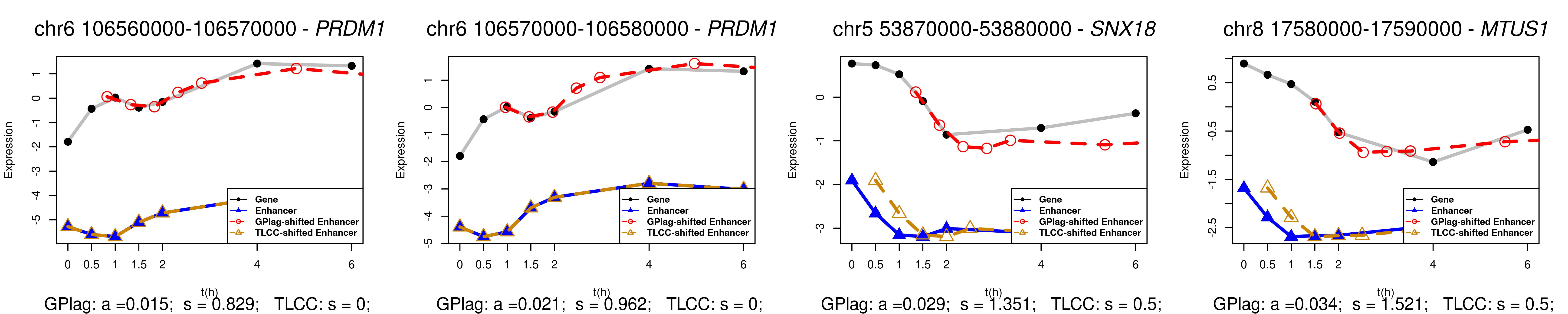
The lack of statistical significance observed in DTW-based methods may be due to the limited information available for alignment because of the small number of observations. Additionally, with irregularly spaced time points, TLCC might introduce bias when estimating time lag and coefficients. Given the constraint of TLCC, which can only generate time lag estimates from the observed time points, its performance was compromised when applied to this dataset with irregular time gaps (Figure 5). However, GPlag, by estimating a continuous time lag, was able to identify lags that restored strong similarity between the pairwise time series.
Thirdly, to evaluate if our candidate enhancer-promoter pairs were detected as having a functional relationship in an orthogonal experimental data type, we downloaded the genomic locations of response expression quantitative trait loci (response eQTL) found in human macrophages exposed to IFNγ (Alasoo et al., 2018) (that is, using one of the two stimuli used in the Reed et al. (2022) experiment, and in the same cell type). Because the number of eQTLs was small compared to the number of enhancers, we used a relatively stringent threshold to label a putative functional enhancer-promoter pair: we split the candidate enhancer-promoter pairs into groups according to posterior mean correlation (). There were 74 H3K27ac peaks overlapping with macrophage response eQTL, among which 12 pairs were in our defined candidate enhancer-promoter pair sets. Therefore, there was a significant enrichment of our candidate enhancer-promoter pairs to eQTLs ( test ) futher suggesting the relevance of the enhancer-promoter pairs highly ranked by GPlag.
6 Discussion
GPlag is a flexible and interpretable model specifically designed for irregular time series with limited time points that exhibit lead-lag effects, a scenario often encountered in biology, which inspired its development. These irregularities can be caused by missing values or study design restrictions. We believe that our method’s adaptability renders it valuable for time series applications in various areas such as longitudinal gene expression, epigenetics, proteomics, cytometry, and microbiome studies. It can be applied to a variety of problems including but not limited to ranking or clustering time series based on the degree of lead-lag effects, and interpolation or forecasting. The core feature of our methodology is the transform of the multi-output GP into a single-output GP, which facilitates the identification of parameters. This approach is grounded in theoretical support, affirming its validity as a covariance kernel for GP. This transform leverages the shared information among time series and enables simultaneous modeling of the time lag parameter and dissimilarity parameters , thereby achieving desirable interpretability and expanding the application of the model. Additionally, our model can be extended to accommodate multiple time series, beyond just pairwise time series, enhancing its applicability and versatility.
The work here suggests some exciting future directions. First, when the sample size is small, the choice of the kernel is crucial in GP models. The extension to a non-stationary kernel allows for more flexibility when modelling non-stationary time series with more heterogeneity. The two main challenges are to find a valid non-stationary kernel with interpretable parameters and perform efficient and effective statistical inference. On the other hand, for time series data with large , i.e., dense time points, the vanilla GP is computationally expensive with complexity (Rasmussen, 2004). In this situation, we can apply scalable GP methods such as nearest neighbor Gaussian processes (NNGP, Datta et al. (2016)) or variational inference GP (Tran et al., 2015) to reduce the complexity to for large datasets. In addition, incorporating additional parameters, such as varying the variance and lengthscale across different time series, could potentially enhance model performance. Finally, the question of whether the parameters in Theorem 3 can be consistently estimated remains open. Even for simpler kernels such as the Matérn, consistent estimators for identifiable parameters (e.g., and ) were only recently developed (Loh et al., 2021; Loh and Sun, 2023). For more complex kernels, like the ones proposed in this paper, constructing consistent estimators is an open and challenging problem.
References
- Alasoo et al. (2018) Alasoo, K., J. Rodrigues, S. Mukhopadhyay, A. J. Knights, A. L. Mann, K. Kundu, C. Hale, G. Dougan, and D. J. Gaffney (2018). Shared genetic effects on chromatin and gene expression indicate a role for enhancer priming in immune response. Nature genetics 50(3), 424–431.
- Apanasovich and Genton (2010) Apanasovich, T. V. and M. G. Genton (2010). Cross-covariance functions for multivariate random fields based on latent dimensions. Biometrika 97(1), 15–30.
- Bachoc et al. (2022) Bachoc, F., E. Porcu, M. Bevilacqua, R. Furrer, and T. Faouzi (2022). Asymptotically equivalent prediction in multivariate geostatistics. Bernoulli 28(4), 2518–2545.
- Bacry et al. (2013) Bacry, E., S. Delattre, M. Hoffmann, and J.-F. Muzy (2013). Some limit theorems for hawkes processes and application to financial statistics. Stochastic Processes and their Applications 123(7), 2475–2499.
- Bennett et al. (2022) Bennett, S., M. Cucuringu, and G. Reinert (2022). Lead–lag detection and network clustering for multivariate time series with an application to the us equity market. Machine Learning, 1–42.
- Berndt and Clifford (1994) Berndt, D. J. and J. Clifford (1994). Using dynamic time warping to find patterns in time series. In KDD workshop, Volume 10, pp. 359–370. Seattle, WA, USA:.
- Bingham et al. (2019) Bingham, E., J. P. Chen, M. Jankowiak, F. Obermeyer, N. Pradhan, T. Karaletsos, R. Singh, P. A. Szerlip, P. Horsfall, and N. D. Goodman (2019). Pyro: Deep universal probabilistic programming. J. Mach. Learn. Res. 20, 28:1–28:6.
- Blondel et al. (2021) Blondel, M., A. Mensch, and J.-P. Vert (2021). Differentiable divergences between time series. In International Conference on Artificial Intelligence and Statistics, pp. 3853–3861. PMLR.
- Byrd et al. (1995) Byrd, R. H., P. Lu, J. Nocedal, and C. Zhu (1995). A limited memory algorithm for bound constrained optimization. SIAM Journal on scientific computing 16(5), 1190–1208.
- Cressie and Huang (1999) Cressie, N. and H.-C. Huang (1999). Classes of nonseparable, spatio-temporal stationary covariance functions. Journal of the American Statistical association 94(448), 1330–1339.
- Cuturi and Blondel (2017) Cuturi, M. and M. Blondel (2017). Soft-dtw: a differentiable loss function for time-series. In International conference on machine learning, pp. 894–903. PMLR.
- Da Fonseca and Zaatour (2017) Da Fonseca, J. and R. Zaatour (2017). Correlation and lead–lag relationships in a hawkes microstructure model. Journal of Futures Markets 37(3), 260–285.
- Datta et al. (2016) Datta, A., S. Banerjee, A. O. Finley, and A. E. Gelfand (2016). Hierarchical nearest-neighbor Gaussian process models for large geostatistical datasets. Journal of the American Statistical Association 111(514), 800–812.
- Davis et al. (2022) Davis, E. S., W. Mu, S. Lee, M. G. Dozmorov, M. I. Love, and D. H. Phanstiel (2022). matchranges: generating null hypothesis genomic ranges via covariate-matched sampling. bioRxiv.
- De Luca and Pizzolante (2021) De Luca, G. and F. Pizzolante (2021). Detecting leaders country from road transport emission time-series. Environments 8(3).
- Ding and Bar-Joseph (2020) Ding, J. and Z. Bar-Joseph (2020). Analysis of time-series regulatory networks. Current Opinion in Systems Biology 21, 16–24.
- Dudley (1989) Dudley, R. M. (1989). Real analysis and probability (wadsworth & brooks/cole: Pacific grove, ca). Mathematical Reviews 441.
- Dürichen et al. (2014) Dürichen, R., M. A. Pimentel, L. Clifton, A. Schweikard, and D. A. Clifton (2014). Multitask gaussian processes for multivariate physiological time-series analysis. IEEE Transactions on Biomedical Engineering 62(1), 314–322.
- Faryabi et al. (2008) Faryabi, B., G. Vahedi, J.-F. Chamberland, A. Datta, and E. R. Dougherty (2008). Optimal constrained stationary intervention in gene regulatory networks. EURASIP Journal on Bioinformatics and Systems Biology 2008, 1–10.
- Feng et al. (2021) Feng, Z., J. A. Sivak, and A. K. Krishnamurthy (2021). Two-stream attention spatio-temporal network for classification of echocardiography videos. In 2021 IEEE 18th International Symposium on Biomedical Imaging (ISBI), pp. 1461–1465. IEEE.
- Fulco et al. (2019) Fulco, C. P., J. Nasser, T. R. Jones, G. Munson, D. T. Bergman, V. Subramanian, S. R. Grossman, R. Anyoha, B. R. Doughty, T. A. Patwardhan, et al. (2019). Activity-by-contact model of enhancer–promoter regulation from thousands of CRISPR perturbations. Nature genetics 51(12), 1664–1669.
- Gardner et al. (2018) Gardner, J., G. Pleiss, K. Q. Weinberger, D. Bindel, and A. G. Wilson (2018). Gpytorch: Blackbox matrix-matrix gaussian process inference with gpu acceleration. Advances in neural information processing systems 31.
- Gelfand et al. (2010) Gelfand, A. E., P. Diggle, P. Guttorp, and M. Fuentes (2010). Handbook of spatial statistics. CRC press.
- Genton and Kleiber (2015) Genton, M. G. and W. Kleiber (2015). Cross-covariance functions for multivariate geostatistics.
- Gerstein et al. (2010) Gerstein, M. B., Z. J. Lu, E. L. Van Nostrand, C. Cheng, B. I. Arshinoff, T. Liu, K. Y. Yip, R. Robilotto, A. Rechtsteiner, K. Ikegami, et al. (2010). Integrative analysis of the caenorhabditis elegans genome by the modencode project. Science 330(6012), 1775–1787.
- Gneiting (2002) Gneiting, T. (2002). Nonseparable, stationary covariance functions for space–time data. Journal of the American Statistical Association 97(458), 590–600.
- Gneiting et al. (2010) Gneiting, T., W. Kleiber, and M. Schlather (2010). Matérn cross-covariance functions for multivariate random fields. Journal of the American Statistical Association 105(491), 1167–1177.
- Harzallah and Sadourny (1997) Harzallah, A. and R. Sadourny (1997). Observed lead-lag relationships between indian summer monsoon and some meteorological variables. Climate dynamics 13, 635–648.
- Hoffmann et al. (2013) Hoffmann, M., M. Rosenbaum, and N. Yoshida (2013). Estimation of the lead-lag parameter from non-synchronous data.
- Hubert and Arabie (1985) Hubert, L. and P. Arabie (1985). Comparing partitions. Journal of classification 2(1), 193–218.
- Ito and Nakagawa (2020) Ito, K. and K. Nakagawa (2020). Naples; mining the lead-lag relationship from non-synchronous and high-frequency data. arXiv preprint arXiv:2002.00724.
- Ito and Sakemoto (2020) Ito, K. and R. Sakemoto (2020). Direct estimation of lead–lag relationships using multinomial dynamic time warping. Asia-Pacific Financial Markets 27(3), 325–342.
- Kaufman and Shaby (2013) Kaufman, C. and B. A. Shaby (2013). The role of the range parameter for estimation and prediction in geostatistics. Biometrika 100(2), 473–484.
- Kazlauskaite et al. (2019) Kazlauskaite, I., C. H. Ek, and N. Campbell (2019). Gaussian process latent variable alignment learning. In The 22nd International Conference on Artificial Intelligence and Statistics, pp. 748–757. PMLR.
- Kingma and Ba (2014) Kingma, D. P. and J. Ba (2014). Adam: A method for stochastic optimization. arXiv preprint arXiv:1412.6980.
- Krijger and De Laat (2016) Krijger, P. H. L. and W. De Laat (2016). Regulation of disease-associated gene expression in the 3d genome. Nature reviews Molecular cell biology 17(12), 771–782.
- Leroy et al. (2022) Leroy, A., P. Latouche, B. Guedj, and S. Gey (2022). Magma: inference and prediction using multi-task gaussian processes with common mean. Machine Learning 111(5), 1821–1849.
- Leroy et al. (2023) Leroy, A., P. Latouche, B. Guedj, and S. Gey (2023). Cluster-specific predictions with multi-task gaussian processes. Journal of Machine Learning Research.
- Li (2022) Li, C. (2022). Bayesian fixed-domain asymptotics for covariance parameters in a Gaussian process model. The Annals of Statistics 50(6), 3334–3363.
- Li et al. (2021) Li, D., A. Jones, S. Banerjee, and B. E. Engelhardt (2021). Multi-group Gaussian processes. arXiv preprint arXiv:2110.08411.
- Li et al. (2023) Li, D., W. Tang, and S. Banerjee (2023). Inference for Gaussian processes with Matérn covariogram on compact riemannian manifolds. Journal of Machine Learning research.
- Lieberman-Aiden et al. (2009) Lieberman-Aiden, E., N. L. van Berkum, L. Williams, M. Imakaev, T. Ragoczy, A. Telling, I. Amit, B. R. Lajoie, P. J. Sabo, M. O. Dorschner, et al. (2009). Comprehensive mapping of long-range interactions reveals folding principles of the human genome. Science 326(5950), 289–293.
- Loh and Sun (2023) Loh, W.-L. and S. Sun (2023). Estimating the parameters of some common gaussian random fields with nugget under fixed-domain asymptotics. Bernoulli 29(3), 2519–2543.
- Loh et al. (2021) Loh, W.-L., S. Sun, and J. Wen (2021). On fixed-domain asymptotics, parameter estimation and isotropic gaussian random fields with matérn covariance functions. The Annals of Statistics 49(6), 3127–3152.
- Love et al. (2014) Love, M. I., W. Huber, and S. Anders (2014). Moderated estimation of fold change and dispersion for RNA-seq data with DESeq2. Genome biology 15(12), 1–21.
- Lu et al. (2021) Lu, J., B. Dumitrascu, I. C. McDowell, B. Jo, A. Barrera, L. K. Hong, S. M. Leichter, T. E. Reddy, and B. E. Engelhardt (2021). Causal network inference from gene transcriptional time-series response to glucocorticoids. PLoS computational biology 17(1), e1008223.
- Mikheeva et al. (2022) Mikheeva, O., I. Kazlauskaite, A. Hartshorne, H. Kjellström, C. H. Ek, and N. Campbell (2022). Aligned multi-task gaussian process. In International Conference on Artificial Intelligence and Statistics, pp. 2970–2988. PMLR.
- Moore et al. (2020) Moore, J. E., M. J. Purcaro, H. E. Pratt, C. B. Epstein, N. Shoresh, J. Adrian, T. Kawli, C. A. Davis, A. Dobin, R. Kaul, et al. (2020). Expanded encyclopaedias of dna elements in the human and mouse genomes. Nature 583(7818), 699–710.
- Rasmussen (2004) Rasmussen, C. E. (2004). Gaussian processes in machine learning. Springer.
- Reed et al. (2022) Reed, K. S., E. S. Davis, M. L. Bond, A. Cabrera, E. Thulson, I. Y. Quiroga, S. Cassel, K. T. Woolery, I. Hilton, H. Won, et al. (2022). Temporal analysis suggests a reciprocal relationship between 3d chromatin structure and transcription. Cell reports 41(5), 111567.
- Rehfeld et al. (2011) Rehfeld, K., N. Marwan, J. Heitzig, and J. Kurths (2011). Comparison of correlation analysis techniques for irregularly sampled time series. Nonlinear Processes in Geophysics 18(3), 389–404.
- Runge et al. (2019) Runge, J., P. Nowack, M. Kretschmer, S. Flaxman, and D. Sejdinovic (2019). Detecting and quantifying causal associations in large nonlinear time series datasets. Science advances 5(11), eaau4996.
- Schoenfelder and Fraser (2019) Schoenfelder, S. and P. Fraser (2019). Long-range enhancer–promoter contacts in gene expression control. Nature Reviews Genetics 20(8), 437–455.
- Shannon (1948) Shannon, C. E. (1948). A mathematical theory of communication. The Bell System Technical Journal 27(3), 379–423.
- Shen (2015) Shen, C. (2015). Analysis of detrended time-lagged cross-correlation between two nonstationary time series. Physics Letters A 379(7), 680–687.
- Skoura (2019) Skoura, A. (2019). Detection of lead-lag relationships using both time domain and time-frequency domain; an application to wealth-to-income ratio. Economies 7(2), 28.
- Stein (1999) Stein, M. L. (1999). Interpolation of spatial data: some theory for kriging. Springer Science & Business Media.
- Strehl and Ghosh (2002) Strehl, A. and J. Ghosh (2002). Normalized mutual information clustering. Journal of Machine Learning Research 3(Feb), 583–617.
- Strober et al. (2019) Strober, B., R. Elorbany, K. Rhodes, N. Krishnan, K. Tayeb, A. Battle, and Y. Gilad (2019). Dynamic genetic regulation of gene expression during cellular differentiation. Science 364(6447), 1287–1290.
- Tran et al. (2015) Tran, D., R. Ranganath, and D. M. Blei (2015). The variational Gaussian process. arXiv preprint arXiv:1511.06499.
- Wang et al. (2017) Wang, D., J. Tu, X. Chang, and S. Li (2017). The lead–lag relationship between the spot and futures markets in china. Quantitative Finance 17(9), 1447–1456.
- Whalen et al. (2016) Whalen, S., R. M. Truty, and K. S. Pollard (2016). Enhancer–promoter interactions are encoded by complex genomic signatures on looping chromatin. Nature genetics 48(5), 488–496.
- Wu et al. (2010) Wu, D., Y. Ke, J. X. Yu, P. S. Yu, and L. Chen (2010). Detecting leaders from correlated time series. In Database Systems for Advanced Applications: 15th International Conference, DASFAA 2010, Tsukuba, Japan, April 1-4, 2010, Proceedings, Part I 15, pp. 352–367. Springer.
- Zhang (2004) Zhang, H. (2004). Inconsistent estimation and asymptotically equal interpolations in model-based geostatistics. Journal of the American Statistical Association 99(465), 250–261.
- Zhu and Gallego (2021) Zhu, J. and B. Gallego (2021). Evolution of disease transmission during the covid-19 pandemic: patterns and determinants. Scientific reports 11(1), 1–9.
Appendix A Additional covariance functions for GPlag
All equations below can serve as covariance functions for GPlag, where measures the spatial variance, measures the group dissimilarity, measures the time lag, measures the range/decay, measures the separability, and measures the smoothness of sample path. is the modified Bessel function of the second kind with degree .
| (S1) | ||||
| (S2) | ||||
| (S3) | ||||
| (S4) | ||||
| (S5) |
As an illustration, Equation S1 is the product of a kernel in Gneiting family with , in Corollary 1 with , and a simple kernel ; Equation S2 is a special case of Equation S1 when . Moreover, if we set , it becomes LExp; Equation S3 can be derived by setting , . Equation S4 can be derived by setting , . Equation S5 is not in Gneiting family, but from Cressie and Huang (1999), who proposed another spectral density based construction for nonseparable spatiotemporal kernels.
In particular, when there are only two time series, the above kernels can be simplified by replacing by and reparameterizing .
A.1 Proof of Theorem 1 and 2
Lemma 1.
Let be a semi-stationary kernel on , where , then the induced kernel defined as
| (S6) |
is positive definite, and thus serves as a covariance kernel for a GP, where =0, measures the time lag with respect to the first time series.
Proof.
It suffices to show that given any set of observations , the covariance matrix is positive definite. We start with a “fake” set of observations, denoted by induced by defined as By the definition of , we observe that
where is the covariance matrix derived from , a positive definite kernel, evaluated on the “fake” set of observations, hence is positive definite. As a result, is positive definite for any time lags . ∎
Theorem 1 can be proved by setting and .
Theorem 2 can be proved by setting as
A.2 Proof of Theorem 3
A powerful tool to study equivalence of Gaussian processes is the spectral density:
Definition 7.
The spectral density associated with stationary Gaussian process in domain is defined as
Remark 1.
There are multiple commonly used definitions for spectral density. For example, is sometimes replaced by and/or without . Throughout this article, we stick to the above definition and omit some absolute multiplicative constants for simplicity.
The following lemma provides the spectral densities of the kernels introduced in Section 2.
Lemma 2.
The spectral densities of LRBF, LExp and LMat and are given by
Proof.
First we calculate the spectral density of LRBF. When , the kernel becomes standard RBF kernel, so the spectral density is given by (Stein, 1999):
When , we replace in by and due to the time shifting property of Fourier transform, we have
.
Then we move to LMat. Similarly, first let , the kernel comes standard Matérn kernel and the spectral density is (Stein, 1999)
For arbitrary and , by the same trick, we have
The spectral density of LExp is obtained by setting in the above equation. ∎
Then we introduce a test, known as the integral test, to determine whether two GPs are equivalent based on their spectral densities. We start with classical GPs on .
Lemma 3 (Integral test for univariate GP(Stein, 1999)).
Let and be spectral densities of two GPs and on domain . Then if
-
1.
There exists such that is bounded away from and as .
-
2.
There exists such that .
Lemma 3 is not directly applicable to our GPlags since our domain is where is the index set of time series. However, a GPlag is equivalent to a multivariate GP with outputs, defined as below:
Definition 8.
A -variate Gaussian process is characterized by its cross-covariance function .
Lemma 4 (Equivalence between GPlags and multivariate GPs Li et al. (2021)).
A -group GPlag on is equivalent to a -variate GP on , where and are related by the following equation:
The above Lemma connects multivariate time series and multiple time series.
Let and be two LMat kernels with parameters and . We first simply the notation as , , , then we have
Observe that is independent of and , and is bounded away from and as . Then we introduce a test to determined whether two GPlags are equivalence.
Lemma 5 (Integral test for multivariate GPs tailored for LMat (Bachoc et al., 2022)).
Let and be spectral matrices of two LMats and , then if there exists such that
Now we can prove Theorem 3.
Proof of Theorem 3.
Observe that
As a result, if and only if
| (S7) |
Since Equation (S7) holds for any , we set certain parameters to special values to isolate conditions on certain parameters. First we let so that and . As a result, Equation (S7) becomes
| (S8) |
Then let , and plug Equation (S8) into Equation (S7), we have
| (S9) |
Finally, plug Equation (S8) and (S9) into Equation (S7), we have , that is, . Recall that by the definition, so we let to get
| (S10) |
To show finite nature of the integral necessitating the condition of (S7), we assume and , i.e., there are only two time series with LExp kernel. In this situation, it suffices to show that if , then .
First, we assume that and , but . Let be an orthonormal basis of the Hilbert space generated by . Let , so we have and by the first half of the proof of Theorem 3. So it suffices to show , which differs only by a multiplicative constant, . As a result, . By Ibragimov and Rozanov (2012, p.72), we conclude that .
Similarly, when , we can prove the same result with ; while when , the corresponding . ∎
A.3 Detailed algorithm
Algorithm 1 and Algorithm 2 illustrates how to calculate the MLE for pairwise and three time series separately.
Algorithm 3 illustrates the realization of the Bayesian inference procedure.
where denotes the inverse gamma distribution and denotes the normal distribution, , , , are hyper-parameters in the prior.
Appendix B Additional experimental details
B.1 Simulation
Parameter Estimation and Inference The variable with various sample size was generated within the range (-50, 50), and a random variation was added by sampling from a uniform distribution with a range of . Three kernels were all served as a covariance function to generate pairwise time series from Gaussian process(GP) with , , set to . When fitting GPlag, the parameters , , were initialized with 1, 1, 1, respectively. For both GPlag and Lead-Lag methods, the upper bound for the time lag was set to 4. The maximum likelihood estimation (MLE) was obtained using the L-BFGS-B algorithm. We plot the MLE of and , as well as (Figure S1). The value of closely matches its true value, aligning with the theoretical predictions discussed in Theorem Theorem 3. Additionally, as increases, the variance decreases, demonstrating the consistency of the MLE.
Furthermore, to evaluate the method’s performance across different lengthscales , and to examine their influence on the estimates of and , we simulate for using the LExp kernel. The results, summarized in the Figure S2, indicate that the value of does influence model optimization. Nonetheless, MLE of both and converge to their true values as the sample size increases.


Prediction For the process that time series generated from the kernel LExp in Equation 3, the variable with was generated within the range (-25, 25), and a random variation was added by sampling from a uniform distribution with a range of . For the linear process with non-Gaussian noise, the variable with was generated within the range (0, 100) with . 50% data were randomly sampled as training sets in one time series, and the corresponding positions in the other time series were also treated as training sets. The remaining 50% data were treated as testing sets. The initial, lower, and upper bound for the time lag was set to 1, -1, 5, respectively. The maximum likelihood estimation (MLE) was obtained using the L-BFGS-B algorithm.

Clustering or Ranking Time Series based on dissimilarity to target time series The variable with for 10 time series (target time series + other 9 time series) was generated regularly from (-2, 2). When fitting GPlag, the parameters , , were initialized with 1, 1, 0, respectively. The lower and upper bound for the time lag was set to -1 and 4, respectively. The maximum likelihood estimation (MLE) was obtained using the L-BFGS-B algorithm. We also replicated this experiment using LRBF and LMat kernels. For both kernels, the ARI and NMI scores were 1 (same as LExp kernel), and the inferred values of were again clearly separated into three distinct clusters Figure S4.

Visual example of kernels
To better help the reader understand and choose the appropriate kernel, here we simulate data from LExp, LMat, and LRBF with various parameter. The simulated sample paths are shown in the following figures. The figures clearly demonstrate that a smaller indicates higher similarity between nearby points, while a smaller reflects greater similarity between the two time series.


B.2 Real-world applications
In order to understand how enhancers regulate gene transcription, Reed et al. (2022) evaluated human macrophage activation after stimulating macrophage with LPS and interferon-gamma (IFNγ). The data were collected at seven irregularly-spaced time points (0, 0.5, 1, 1.5, 2, 4, 6 h). At each time point, the 3D chromatin structure was profiled using in situ Hi-C, putative enhancer activity using chromatin immunoprecipitation sequencing (ChIP-seq) targeting histone 3 lysine 27 acetylation (H3K27ac), chromatin accessibility using assay for transposase-accessible chromatin using sequencing (ATAC-seq), and gene expression using RNA sequencing (RNA-seq). Hi-C scale was indicated in KR-normalized counts, H3K27ac and RNA-seq using variance stabilizing transformation (VST) from the DESeq2 package (Love et al., 2014).
We characterize synchronization between activity at enhancers and transcription at promoters allowing for time lags. Time lags help to better model potential causal relationships between chromatin accessibility and gene transcription. Usually, changes in acetylation at distal enhancers precede changes in gene expression (Reed et al., 2022), so we assume the time lag parameter is positive and set its upper bound to 2h. In total, we have 22,813 enhancer and gene pairs. Since we believe stimulation would activate enhancer and gene changes, we removed the gene and enhancers whose range of normalized expression is smaller than 1. 4,776 non-static pairs remained for analysis. For Hi-C value, expected counts are determined using distance decay from the diagonal and the total read depth of the bins, so the resulting value is independent of distance.
The GPlag model employed the LRBF kernel in Equation 2, with time initialization obtained from TLCC and parameter initialization from GP modeling on gene expression. The optimization process utilized the L-BFGS-B algorithm.