Gauge theory and mixed state criticality

Open quantum systems are quantum systems that interact with the environment, making them ubiquitous in nature. While such interactions may be unwanted in certain practical applications, they can also be harnessed for beneficial outcomes when actively controlled. In order to do so, it is important to find unique phenomena that have no direct counterparts in closed systems. For example, entangled states can be prepared by using dissipation and measurements [1, 2, 3, 4, 5, 6, 7, 8]; Topological phases and phenomena unique to open and non-hermitian quantum systems have also been classified [9, 10, 11]; Quantum many-body systems under monitoring undergo a measurement-induced phase transition between distinct dynamical phases [12]; Furthermore, recent studies have explored the fate of topological phases at finite temperature and under decoherence [13, 14, 15, 16, 17], as well as topological order intrinsic to mixed states [18, 19, 20]. With these exciting developments at hand, it would be important to have a unified method to understand and expand the landscape of those inherently open phenomena and phases of matter.

The notion of symmetry is crucial in understanding the behavior of many-body phases. Indeed, symmetry has proven useful in classifying phases of matter of closed systems at equilibrium, such as spontaneous symmetry breaking (SSB) or symmetry-protected topological (SPT) phases [21, 22, 23, 24, 25, 26, 27, 28, 29]. For open quantum systems, such a program is even more interesting due to the fact that symmetry can act from the left or the right on the mixed-state density matrix. It is customary and convenient to classify the symmetry of the mixed state into two classes, strong and weak symmetries. In the case of strong symmetry, the density matrix is (projectively) invariant under the action of the left and the right symmetry independently, while in the weak symmetry case, only under the diagonal subgroup [30]. Put differently, the former is defined by $U\rho=\rho U^{{\dagger}}=\rho$, and the latter, less stringently, by $U\rho U^{\dagger}=\rho$, where $U$ is a unitary operator acting on the system’s Hilbert space, and $\rho$ the density matrix ¹¹1All up to an overall phase factor accommodating the projective representation. Note also that we do not consider non-unitary symmetries in this Letter.. We further define the spontaneous symmetry breaking of strong and weak symmetries by using off-diagonal long-range order, which will be discussed later in the main body of the text. This distinction enables us to explore broader landscapes of quantum phases inherent to open quantum systems, such as SSB, phase transitions [32, 33, 34] or SPT orders [35, 36, 37, 38, 39, 40, 41, 42, 43] Lieb-Schultz-Mattis type theorems and quantum anomalies for open quantum systems have also been formulated in [44, 45, 46, 47].

In this work, we present a unifying approach to classify phases of matter that are inherently open. Concretely, we introduce a systematic way to construct various spontaneous symmetry-breaking phases of open quantum systems, including strong-to-weak SSB (SWSSB) phases, by starting from the ground state phase diagram of lattice gauge theory models which are closed. Our construction also allows us to study criticalities between them, including those that support gapless symmetry-protected topological (gSPT) order [48, 49, 50, 51, 52, 53, 54, 55, 56, 57, 58, 59, 60, 61, 62, 63, 64, 65, 66, 67, 68]. By leveraging the structure of lattice gauge theories, we provide a framework for studying quantum operations between different mixed quantum phases, which provides valuable insights in open quantum many-body systems.

Let us start from lattice models with emergent gauge fields at low energy, such as the Hamiltonian lattice gauge theory [69, 70]. We in particular focus on the $\mathbb{Z}_{2}$ lattice gauge theory in one spatial dimension as a concrete example, whose Hamiltonian we denote by $H$. Its degrees of freedom are composed of matter and gauge fields, which live on vertices (i.e., sites) and links, respectively. We denote the Hilbert space of the theory (before imposing the Gauss law constraint, to be introduced later) by $\mathcal{H}\equiv\bigotimes_{j}\left(\mathcal{H}_{v,j}\otimes\mathcal{H}_{l,j+1/2}\right)$, where ${\cal H}_{v,j}$ is the matter Hilbert space at site $j$, while ${\cal H}_{l,j+1/2}$ is the $\mathbb{Z}_{2}$ gauge field Hilbert space living on the link connecting sites $j$ and $j+1$, both of which are two-dimensional. We denote the Pauli operators on ${\cal H}_{v,j}$ as $X_{j}$, $Y_{j}$ and $Z_{j}$, and on ${\cal H}_{l,j}$ as $\sigma_{j}^{x}$, $\sigma_{j}^{y}$ and $\sigma_{j}^{z}$.

Physical states in the $\mathbb{Z}_{2}$ gauge theory, as in any gauge theories, satisfy the Gauss law constraint. This is a constraint that $\sigma^{z}_{j-1/2}X_{j}\sigma^{z}_{j+1/2}=1$ for any physical states $\ket{\psi}$, i.e.,

for all $j$. This can indeed be interpreted as gauging the $\mathbb{Z}_{2}$ symmetry of the matter theory – The would-be $\mathbb{Z}_{2}$ global symmetry of the matter theory generated by $\prod_{j}X_{j}$ (which flips the spin at the vertices all at once) acts on physical states trivially as $\prod_{j}X_{j}=\prod_{j}G_{j}$. (Throughout the paper, we will work with periodic boundary conditions unless stated otherwise.)

One can also impose such a constraint energetically in the UV lattice model, by explicitly adding $-K\sum_{j}G_{j}$ to the Hamiltonian – If $K$ is large enough, we get the same ground state as the original $\mathbb{Z}_{2}$ gauge theory. In the following, we will call this procedure the effective gauging and the resulting theory as the effective gauge theory [71, 72, 68, 73, 74]. As it has been proven useful in constructing lattice models with SPT orders [21, 22, 23, 24, 25, 26, 27, 28, 29] or gapless topological phases [48, 49, 50, 51, 52, 53, 54, 55, 56, 57, 58, 59, 60, 61, 62, 63, 64, 65, 66, 67, 68] in closed equilibrium systems, we will utilize it to study analogous phases in open quantum systems as well. It also has an advantage over the usual lattice gauge models as there is no need to impose Gauss law and hence all the symmetries are global symmetries.

We are interested in various phases of matter realized in mixed states, obtained by tracing out the matter degrees of freedom in the ground state pure state of lattice gauge theories, since they already exhibit various interesting phases at equilibrium and we expect this to carry over to mixed states. We denote the environment Hilbert space by $\mathcal{H}_{A}$, which is a subspace of $\mathcal{H}_{v}$ on which the symmetry acts faithfully. In our examples below, $\mathcal{H}_{A}=\mathcal{H}_{v}$ in the first example, while in the second and third, $\mathcal{H}_{A}\subsetneq\mathcal{H}_{v}$.

Our claim is that, the operation of taking the partial trace, which is commonly used in studying the phases of the mixed state, can be replaced by quantum channels describing decoherence and gauge fixing (or vice versa):

For a density matrix $\rho$ composed of pure states satisfying the Gauss law, i.e., $G_{j}\rho=\rho G^{{\dagger}}_{j}=\rho$, we have

Here, $\mathcal{E}_{ZZ}$ and $\mathcal{E}_{CZ}$ are quantum operations acting on density matrices defined in the following way,

and

where $\texttt{CZ}_{j,k}$ is the contorolled-Z gate between two qubits. More concretely, we define $\texttt{CZ}_{j,k}$ as $\texttt{CZ}_{j,k}=\mathop{\mathrm{diag}}(1,1,1,-1)$ on the $(\ket{\uparrow_{j},\uparrow_{k}},\ket{\uparrow_{j},\downarrow_{k}},\ket{\downarrow_{j},\uparrow_{k}},\ket{\downarrow_{j},\downarrow_{k}})$ basis system.

Deferring the proof to Supplementary Material, let us now discuss the physical meaning of (2). First of all, what the operation $\rho\mapsto\operatorname{Tr}_{\mathcal{H}_{A}}(\mathcal{E}_{CZ}(\rho))$ achieves is the gauge fixing on each pure state included in $\rho$. This is because $\mathcal{E}_{CZ}$ transforms the Gauss constraint $\sigma^{z}_{j-{1/2}}X_{j}\sigma^{z}_{j+1/2}=1$ to $X_{j}=1$, and hence the matter degrees of freedom are disentangled from the rest. We call this gauge the unitary gauge. (See Supplementary Material for more discussions.) Precisely speaking, the exact disentangling only happens for lattice gauge theories in which the gauge symmetry is manifest in the UV – for effective gauge theories, there would be a term to freeze the matter spin $X_{j}$ to $1$. When such a term becomes larger and larger in the IR, there is an effective disentangling between the matter and the gauge degrees of freedom.

Our main result (2) can be useful in different ways. First of all, we can use it to study the effect of decoherence on $\tilde{\rho}=\mathrm{Tr}_{{\cal H}_{A}}\,\left({\cal E}_{CZ}\,(\rho)\right)$. (Note that $\tilde{\rho}$ is a pure state from the discussion above.) This is useful because $\tilde{\rho}$ can be thought of as the ground state of the new (non-gauge) Hamiltonian $\tilde{H}$, which can be obtained from $H$ algorithmically by gauge fixing and a projection. We will discuss this shortly using examples in the next section.

The claim (2) can also be used to infer properties of the mixed state (reduced) density matrix $\varrho$. For example, it is immediate that $\varrho$ spontaneously breaks the strong $\mathbb{Z}_{2}$ symmetry of flipping the gauge spin. The spontaneous symmetry breaking in this Letter will be defined by using the so-called Rényi-2 correlator [32, 33, 34, 75], such that the spontaneous symmetry breaking happens when

To see this, first notice that $\mathcal{E}_{ZZ}(\tilde{\rho})$ is symmetric under the strong $\mathbb{Z}_{2}$ symmetry as long as $\tilde{\rho}$ is symmetric as well, which is the case for us. Moreover, one can see that two-point correlations are exactly preserved under the operation,

as

Here, $s_{j}\in\{0,1\}$ and the summand for $\{s\}_{j}$ runs over all configurations such that the number of $j$ with $s_{j}=1$ is even. We also see that the Rényi-2 correlations are always nontrivial,

by using the form of $\mathcal{E}_{ZZ}(\rho)$ – The density matrix $\varrho$ breaks the strong $\mathbb{Z}_{2}$ symmetry spontaneously as promised.

Strikingly, if the procedure is applied to gauge theories at criticality, we always end up with some sort of critical points for open systems. In the following, we explore three classes of models with such criticalities.

We first explore the simplest criticality that is intrinsic to mixed states; between SWSSB and SSB phases. As a prime example, we investigate the criticality of the transverse-field Ising (TFI) model. The Hamiltonian for the gauge theory is given by

where $L$ is the total number of lattice sites and we impose the periodic boundary condition, and we take $J>0$ throughout the Letter. In this expression, the model has two $\mathbb{Z}_{2}$ global symmetries generated by $\prod_{j}\sigma^{x}_{j+1/2}$ and $\prod_{j}X_{j}$. Depending on the value of the parameter $J$ the ground state of (11) belongs to three different phases (Table 1). When $J<1$, the first $\mathbb{Z}_{2}$ symmetry is spontaneously broken in the ground state, while the other remains unbroken. When $J>1$, the ground state exhibits the $\mathbb{Z}_{2}\times\mathbb{Z}_{2}$ SPT order. While the model is gapless at $J=1$, it also has a non-trivial string order correlation $\braket{\sigma^{z}_{i-1/2}X_{i}\,\cdots\,X_{i+r}\sigma^{z}_{i+r+1/2}}$. Moreover, this model has a protected edge mode when put on the open boundary. Gapless systems that exhibit these features are known as gapless SPT (gSPT) phases [48, 49].

We now discuss various mixed states obtained from the ground state by tracing the vertex degrees of freedom (Table 2). When tracing out the vertex degrees of freedom, the SSB (SPT) phase becomes the SSB (SWSSB) phase [34]. Therefore, we obtain a critical mixed state between SSB and SWSSB phases, by tracing out the gapped degree of the gSPT state at $J=1$.

Let $\rho_{0}$ be a ground state of $H_{1}$. Then $\widetilde{\rho_{0}}=\operatorname{Tr}_{\mathcal{H}_{A}}\left(\mathcal{E}_{CZ}(\rho_{0})\right)$ is a ground state of the gauge theory in the unitary gauge. Specifically, $\widetilde{\rho_{0}}$ is a ground state of the Hamiltonian

which exhibits the unbroken, gapped phase ($J>1$), the SSB phase ($J<1$), and the Ising criticality separating them ($J=1$). The two-point correlation function of the ground state behaves as

in the thermodynamic limit, where $\Delta$ is the scaling dimension of $\sigma^{z}$ at criticality, while at $J>1$, $m$ is the gap of the system. This correlation remains the same after the $\mathcal{E}_{ZZ}$ operation. On the other hand, as discussed, the Rényi-2 correlators are non-trivial for any $J$. Namely, the $J>1$ phase is mapped to the SWSSB phase under the $\mathcal{E}_{ZZ}$ operation. As for the critical point $J=1$, $\operatorname{Tr}_{\mathcal{H}_{A}}(\rho_{0})=\mathcal{E}_{ZZ}(\widetilde{\rho_{0}})$ exhibits the criticality between SWSSB and SSB phases. We summarize various correlation functions of this model at criticality in Table 3.

In the previous example, we discussed the model that exhibits Ising CFT criticality in the corresponding gauge theory, and such criticality describes the transition between the $\mathbb{Z}_{2}$ SSB phase and the $\mathbb{Z}_{2}$ trivial phase. Let us now discuss a criticality between an SSB phase and a non-trivial SPT phase. Such a criticality is described by a gSPT. As a model for $\mathbb{Z}_{2}$ (effective) gauge theory, we consider the following Hamiltonian:

where $\tau_{j}^{x,y,z}$ are the Pauli matrices, $K_{0}$ is a sufficiently large positive constant, and the last term (positive $K$) is for effective gauging. In the unitary gauge or after implementing $\operatorname{Tr}_{\mathcal{H}_{A}}\left(\mathcal{E}_{CZ}(\cdot)\right)$ operation, the ground state of the model is the same as the following Hamiltonian:

This model is the same as (11), and the critical point $J=1$ separates the SSB and SPT phases (Table 1). Since the last term commutes with the other terms, this term is stabilized at the ground state and gives a gapped sector. Looking at the gapless low-energy sector, this model is described by the Ising CFT. There are two correlators that characterize this critical point. One of them is $\braket{\sigma^{z}_{i}\sigma^{z}_{i+r}}$ and it exhibits algebraic decay which corresponds to the two-point correlation in the Ising CFT, and the other is the string correlator $\braket{\sigma^{z}_{i-1/2}X_{i}\,\cdots\,X_{i+r}\sigma^{z}_{i+r+1/2}}$ that indicates long-range order.

Since operators that consist of the quantum operation $\mathcal{E}_{ZZ}$ commute with the two correlators, these correlations are preserved under the operation. On the other hand, the quantum operation can affect the Rényi-2 correlation for $\sigma^{z}_{i}\sigma^{z}_{i+r}$, and indeed this exhibits long-range order after the operation. We realize that, after taking the partial trace of the ground state of (Criticality between “SWSSB-ASPT” and SSB), $\mathrm{Tr}_{{\cal H}_{A}}\,(\rho)$, we have an interesting mixed state for $J>1$. While $\mathrm{Tr}_{{\cal H}_{A}}\,(\rho)$ exhibits a strong-to-weak SSB order with respect to $\prod_{j}\sigma^{x}_{j+1/2}$, there still be a non-vanishing string correlation $\braket{\sigma^{z}_{i-1/2}X_{i}\,\cdots\,X_{i+r}\sigma^{z}_{i+r+1/2}}$. We note that the other string correlator $\braket{Z_{i}\sigma^{x}_{i+1/2}\,\cdots\,\sigma^{x}_{i+r-1/2}Z_{i+r}}$, which also characterizes the non-trivial SPT phase, no longer exhibits long-range order after the $\mathcal{E}_{ZZ}$ operation. Such a behavior of the two string correlations is one of the hallmarks of average SPT (ASPT) phases [36, 37]. In this sense, the phase for $J>1$ is kind of a “mixture” of SWSSB and ASPT phases. We call this phase SWSSB-ASPT. In summary, the two gapped phases of the ground state of (15) are mapped to the SSB ($J<1$) and SWSSB-ASPT ($J>1$) phases under the quantum operation $\mathcal{E}_{ZZ}$, and at $J=1$ the critical point is mapped to the critical mixed state between them (Table 2). We summarize various correlation functions of this model at criticality in Table 3.

Let us explore a critical model obtained by applying the $\mathcal{E}_{ZZ}$ operation to an intrinsically gapless SPT (igSPT) criticality [50]. Since igSPT models exhibit emergent ’t Hooft anomalies in the IR and such anomalies forbid the existence of unique gapped ground states, such criticality may describe phase transitions between different SSB patterns. Let us consider the model of the effective gauge theory of the form

Here, $K_{0}$ is again a sufficiently large positive constant and $\hat{X}_{j},\hat{Z}_{j}$ are generalized Pauli matrices acting on a $j$-th four-dimensional qudit space and satisfy $\hat{X}_{j}^{4}=\hat{Z}_{j}^{4}=1,\quad\hat{Z}_{j}\hat{X}_{j}=i\hat{X}_{j}\hat{Z}_{j}.$ In the unitary gauge, this model is written as

At $J=1$, this model is known to realize an igSPT phase with a $\mathbb{Z}_{4}\times\mathbb{Z}_{2}$ global symmetry [66, 68]. The $\mathbb{Z}_{4}$ symmetry is generated by $\prod_{j}\hat{X}_{j}$, while the $\mathbb{Z}_{2}$ symmetry is generated by $\prod_{j}\sigma_{j+1/2}^{x}$. When $J<1$, the $\mathbb{Z}_{4}$ symmetry remains unbroken, while the $\mathbb{Z}_{2}$ symmetry is spontaneously broken. When $J>1$, the $\mathbb{Z}_{4}$ symmetry breaks to the $\mathbb{Z}_{2}$ subgroup while the other $\mathbb{Z}_{2}$ global symmetry remains unbroken. Moreover, a non-trivial SPT phase with respect to this unbroken $\mathbb{Z}_{2}\times\mathbb{Z}_{2}$ symmetry is stacked. At $J=1$, the low-energy sector of the model is described by the $U(1)_{4}$ CFT ²²2The $U(1)_{4}$ CFT is Tomonaga-Luttinger liquid with a certain Luttinger parameter.. See Table 1 for the phase diagram. The criticality of the corresponding CFT is captured by two-point correlations e.g. $\braket{\sigma_{i}^{z}\sigma_{i+r}^{z}}$. In addition to such usual CFT correlators, this igSPT is characterized by the string order parameter $\braket{\sigma_{i-1/2}^{z}\hat{X}_{i}^{2}\,\cdots\,\hat{X}_{i+r}^{2}\sigma_{i+r+1/2}^{z}}$. One can see this correlation has an $O(1)$ expectation value because the last term in (17) commutes with the other term, and so it is stabilized at the ground state.

Let us consider the mixed state obtained by applying the operation $\mathcal{E}_{ZZ}$ (Table 2). For $J<1$ where the $\mathbb{Z}_{2}$ symmetry is spontaneously broken, the state is mapped to the same SSB phase. In contrast, for $J>1$, the state is mapped to an SSB phase where the $\mathbb{Z}_{4}$ symmetry breaks down to the diagonal $\mathbb{Z}_{2}$, which hosts an SWSSB-ASPT order, as observed in the previous model. The critical point $J=1$ separates these two phases and exhibits a critical behavior in the correlation $\braket{\sigma_{i}^{z}\sigma_{i+r}^{z}}$, along with a long-range order in the string order correlation $\braket{\sigma_{i-1/2}^{z}\hat{X}_{i}^{2}\cdots\hat{X}_{i+r}^{2}\sigma_{i+r+1/2}^{z}}$. We summarize various correlation functions of this model at criticality in Table 3.

We have seen that ground states of $\mathbb{Z}_{2}$ gauge theories can be interpreted as purified states of the corresponding mixed states. Purification is a common technique to treat mixed states as pure states. On the other hand, mixed states can be mapped to pure states in the doubled Hilbert space in a canonical way by the Choi-Jamiołkowski isomorphism [77, 78]. To see the isomorphism, note that a density matrix is an element of $\operatorname{End}(\mathcal{H})$, and the isomorphism maps the element to $\mathcal{H}\otimes\mathcal{H}^{*}$. For example, a pure state $\ket{\psi}\bra{\psi}$ is mapped to $\ket{\psi}\otimes\ket{\psi}^{*}\in\mathcal{H}\otimes{\cal H}^{*}$. We denote an operator that acts on $\mathcal{H}$ by using the tilde. Let $\rho_{0}$ be a pure state and $\rho=\mathcal{E}_{ZZ}(\rho_{0})$. We denote the doubled state obtained from $\rho(\rho_{0})$ by $|\rho\rangle\!\rangle(|\rho_{0}\rangle\!\rangle)$. Since both $\rho_{0}$ and $\rho$ have the strong $\mathbb{Z}_{2}$ symmetry, the corresponding states $|\rho_{0}\rangle\!\rangle,|\rho\rangle\!\rangle$ have a $\mathbb{Z}_{2}\times\mathbb{Z}_{2}$ symmetry generated by $\prod_{j}\sigma_{j}^{x},\prod_{j}\widetilde{\sigma}_{j}^{x}$.

How can we understand correlations for mixed states in the double state picture? Through a simple calculation, we find that

On the other hand,

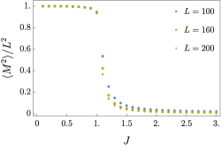
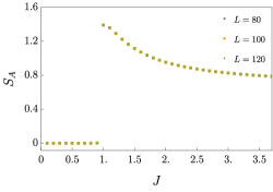
(Table 4). Since the operator $\sigma^{z}_{i}\widetilde{\sigma}^{z}_{i}$ is charged only for the off-diagonal global symmetry, this correlation diagnoses whether the off-diagonal symmetry is spontaneously broken or not. However, as we have already discussed, this Rényi-2 correlator is always non-trivial and so the off-diagonal symmetry is necessarily broken in $|\rho\rangle\!\rangle$. On the other hand, SSB of the diagonal $\mathbb{Z}_{2}$ symmetry is diagnosed by $\langle\!\langle\rho|\sigma^{z}_{i}\sigma^{z}_{i+r}|\rho\rangle\!\rangle$. However, it is proportional to $\operatorname{Tr}(\rho^{2}\sigma^{z}_{i}\sigma^{z}_{i+r})$ and the expectation value depends on the specific model in general. We have numerically calculated the magnetization and entanglement entropies of Model 1 we discussed above (Fig. 1). We found that there is an order one magnetization squared and entanglement entropies obey the area law. In particular, the entanglement entropy is about $2\ln(2)$.

While we have hitherto discussed systems in one spatial dimension, our formulation can be generalized to higher dimensions. Specifically, in a spatial $d$-dimensional system, the Gauss law for the vertex $v$ is imposed to be $X_{v}\prod_{l}\sigma^{z}_{l}\ket{\text{phys}}=+\ket{\text{phys}}$ where $l$ denotes the links adjacent to the vertex. In general, such a gauge theory has a magnetic $\mathbb{Z}_{2}$ $(d-1)$-form symmetry and its charged object, which is a $(d-1)$-dimensional object, is composed of the $Z_{l}$ operators. This object serves as an order parameter for the $(d-1)$-form symmetry. As in the case of $(1+1)d$, mixed states obtained by tracing out the vertex degrees of freedom can be related to a particular quantum channel. This quantum operation exactly preserves the correlations of the order parameter and completely breaks the strong symmetry spontaneously. The idea discussed in this Letter can readily be generalized to other gauge theories such as for finite gauge groups and higher-form gauge symmetries.

In this Letter, we present a method to construct various phases with the spontaneous breaking of strong symmetry. Taking the partial trace is equivalent to applying the quantum operation $\mathcal{E}_{ZZ}$ in the unitary gauge. A key property enabling us to calculate correlation functions is that the “decohering” operator $\mathcal{E}_{ZZ}$ commutes with the order parameter of charged operators for global symmetries. We expect that our construction can be extended to a wider class of lattice models and decoherence channels – we lead it for future work.

One of the merits of our construction is that we can apply various knowledge of gauge theories through the correspondence between gauge theories and mixed states. This can help us to study some aspects of mixed states of matter. For example, we expect we can explore the “duality web” in mixed states, as the web for (topological) gauge theories is already well-studied. In a mixed-state picture, duality operations are replaced by appropriate quantum operations as discussed in e.g. [81, 82].

Note added: While the preparation of the draft was at the final stage, we learned [83] in which some of the strong SSB phases and criticalities in this Letter were also discussed from the perspective of the imaginary time evolution of Lindbladians.

T.A. thanks Kenji Shimomura for useful discussions. T.A. is supported by JST CREST (Grant No. JPMJCR19T2). S.R. is supported by Simons Investigator Grant from the Simons Foundation (Grant No. 566116). M.W. is supported by Grant-in-Aid for JSPS Fellows (Grant No. 22KJ1777) and by MEXT KAKENHI Grant (Grant No. 24H00957).

References

- Diehl et al. [2008] S. Diehl, A. Micheli, A. Kantian, B. Kraus, H. P. Büchler, and P. Zoller, Quantum States and Phases in Driven Open Quantum Systems with Cold Atoms, Nature Physics 4, 878 (2008), arXiv:0803.1482 [quant-ph] .
- Tantivasadakarn et al. [2024] N. Tantivasadakarn, R. Thorngren, A. Vishwanath, and R. Verresen, Long-Range Entanglement from Measuring Symmetry-Protected Topological Phases, Phys. Rev. X 14, 021040 (2024), arXiv:2112.01519 [cond-mat.str-el] .
- Verresen et al. [2021a] R. Verresen, N. Tantivasadakarn, and A. Vishwanath, Efficiently preparing Schrödinger’s cat, fractons and non-Abelian topological order in quantum devices (2021a), arXiv:2112.03061 [quant-ph] .
- Lu et al. [2022] T.-C. Lu, L. A. Lessa, I. H. Kim, and T. H. Hsieh, Measurement as a Shortcut to Long-Range Entangled Quantum Matter, PRX Quantum 3, 040337 (2022), arXiv:2206.13527 [cond-mat.str-el] .
- Lu et al. [2023] T.-C. Lu, Z. Zhang, S. Vijay, and T. H. Hsieh, Mixed-State Long-Range Order and Criticality from Measurement and Feedback, PRX Quantum 4, 030318 (2023), arXiv:2303.15507 [cond-mat.str-el] .
- Foss-Feig et al. [2023] M. Foss-Feig et al., Experimental demonstration of the advantage of adaptive quantum circuits (2023), arXiv:2302.03029 [quant-ph] .
- Iqbal et al. [2024a] M. Iqbal et al., Topological order from measurements and feed-forward on a trapped ion quantum computer, Commun. Phys. 7, 205 (2024a), arXiv:2302.01917 [quant-ph] .
- Iqbal et al. [2024b] M. Iqbal et al., Non-Abelian topological order and anyons on a trapped-ion processor, Nature 626, 505 (2024b), arXiv:2305.03766 [quant-ph] .
- Ashida et al. [2021] Y. Ashida, Z. Gong, and M. Ueda, Non-Hermitian physics, Adv. Phys. 69, 249 (2021), arXiv:2006.01837 [cond-mat.mes-hall] .
- Okuma and Sato [2023] N. Okuma and M. Sato, Non-Hermitian Topological Phenomena: A Review, Ann. Rev. Condensed Matter Phys. 14, 83 (2023), arXiv:2205.10379 [cond-mat.mes-hall] .
- Bergholtz et al. [2021] E. J. Bergholtz, J. C. Budich, and F. K. Kunst, Exceptional topology of non-hermitian systems, Rev. Mod. Phys. 93, 015005 (2021).
- Fisher et al. [2023] M. P. A. Fisher, V. Khemani, A. Nahum, and S. Vijay, Random Quantum Circuits, Ann. Rev. Condensed Matter Phys. 14, 335 (2023), arXiv:2207.14280 [quant-ph] .
- Dennis et al. [2002] E. Dennis, A. Kitaev, A. Landahl, and J. Preskill, Topological quantum memory, J. Math. Phys. 43, 4452 (2002), arXiv:quant-ph/0110143 .
- Lee et al. [2022] J. Y. Lee, Y.-Z. You, and C. Xu, Symmetry protected topological phases under decoherence (2022), arXiv:2210.16323 [cond-mat.str-el] .
- Fan et al. [2024] R. Fan, Y. Bao, E. Altman, and A. Vishwanath, Diagnostics of Mixed-State Topological Order and Breakdown of Quantum Memory, PRX Quantum 5, 020343 (2024), arXiv:2301.05689 [quant-ph] .
- Bao et al. [2023] Y. Bao, R. Fan, A. Vishwanath, and E. Altman, Mixed-state topological order and the errorfield double formulation of decoherence-induced transitions (2023), arXiv:2301.05687 [quant-ph] .
- Chen and Grover [2024] Y.-H. Chen and T. Grover, Unconventional topological mixed-state transition and critical phase induced by self-dual coherent errors, Phys. Rev. B 110, 125152 (2024), arXiv:2403.06553 [quant-ph] .
- Sohal and Prem [2024] R. Sohal and A. Prem, A Noisy Approach to Intrinsically Mixed-State Topological Order (2024), arXiv:2403.13879 [cond-mat.str-el] .
- Ellison and Cheng [2024] T. Ellison and M. Cheng, Towards a classification of mixed-state topological orders in two dimensions (2024), arXiv:2405.02390 [cond-mat.str-el] .
- Wang et al. [2023] Z. Wang, Z. Wu, and Z. Wang, Intrinsic Mixed-state Quantum Topological Order (2023), arXiv:2307.13758 [quant-ph] .
- Gu and Wen [2009] Z.-C. Gu and X.-G. Wen, Tensor-Entanglement-Filtering Renormalization Approach and Symmetry Protected Topological Order, Phys. Rev. B 80, 155131 (2009), arXiv:0903.1069 [cond-mat.str-el] .
- Pollmann et al. [2012] F. Pollmann, E. Berg, A. M. Turner, and M. Oshikawa, Symmetry protection of topological phases in one-dimensional quantum spin systems, Phys. Rev. B 85, 075125 (2012), arXiv:0909.4059 [cond-mat.str-el] .
- Pollmann et al. [2010] F. Pollmann, A. M. Turner, E. Berg, and M. Oshikawa, Entanglement spectrum of a topological phase in one dimension, Phys. Rev. B 81, 064439 (2010), arXiv:0910.1811 [cond-mat.str-el] .
- Chen et al. [2011] X. Chen, Z.-C. Gu, and X.-G. Wen, Classification of gapped symmetric phases in one-dimensional spin systems, Phys. Rev. B 83, 035107 (2011), arXiv:1008.3745 [cond-mat.str-el] .
- Schuch et al. [2011] N. Schuch, D. Pérez-García, and I. Cirac, Classifying quantum phases using matrix product states and projected entangled pair states, Phys. Rev. B 84, 165139 (2011), arXiv:1010.3732 [cond-mat.str-el] .
- Chen et al. [2013] X. Chen, Z.-C. Gu, Z.-X. Liu, and X.-G. Wen, Symmetry protected topological orders and the group cohomology of their symmetry group, Phys. Rev. B 87, 155114 (2013), arXiv:1106.4772 [cond-mat.str-el] .
- Levin and Gu [2012] M. Levin and Z.-C. Gu, Braiding statistics approach to symmetry-protected topological phases, Phys. Rev. B 86, 115109 (2012), arXiv:1202.3120 [cond-mat.str-el] .
- Chen et al. [2012] X. Chen, Z.-C. Gu, Z.-X. Liu, and X.-G. Wen, Symmetry-Protected Topological Orders in Interacting Bosonic Systems, Science 338, 1604 (2012), arXiv:1301.0861 [cond-mat.str-el] .
- Senthil [2015] T. Senthil, Symmetry Protected Topological phases of Quantum Matter, Ann. Rev. Condensed Matter Phys. 6, 299 (2015), arXiv:1405.4015 [cond-mat.str-el] .
- Albert and Jiang [2014] V. V. Albert and L. Jiang, Symmetries and conserved quantities in lindblad master equations, Physical Review A 89, 10.1103/physreva.89.022118 (2014).
- Note [1] All up to an overall phase factor accommodating the projective representation. Note also that we do not consider non-unitary symmetries in this Letter.
- Lee et al. [2023] J. Y. Lee, C.-M. Jian, and C. Xu, Quantum Criticality Under Decoherence or Weak Measurement, PRX Quantum 4, 030317 (2023), arXiv:2301.05238 [cond-mat.stat-mech] .
- Lessa et al. [2024a] L. A. Lessa, R. Ma, J.-H. Zhang, Z. Bi, M. Cheng, and C. Wang, Strong-to-Weak Spontaneous Symmetry Breaking in Mixed Quantum States (2024a), arXiv:2405.03639 [quant-ph] .
- Sala et al. [2024] P. Sala, S. Gopalakrishnan, M. Oshikawa, and Y. You, Spontaneous strong symmetry breaking in open systems: Purification perspective, Phys. Rev. B 110, 155150 (2024), arXiv:2405.02402 [quant-ph] .
- de Groot et al. [2022] C. de Groot, A. Turzillo, and N. Schuch, Symmetry Protected Topological Order in Open Quantum Systems, Quantum 6, 856 (2022), arXiv:2112.04483 [quant-ph] .
- Ma and Wang [2023] R. Ma and C. Wang, Average Symmetry-Protected Topological Phases, Phys. Rev. X 13, 031016 (2023), arXiv:2209.02723 [cond-mat.str-el] .
- Ma et al. [2023] R. Ma, J.-H. Zhang, Z. Bi, M. Cheng, and C. Wang, Topological Phases with Average Symmetries: the Decohered, the Disordered, and the Intrinsic (2023), arXiv:2305.16399 [cond-mat.str-el] .
- Zhang et al. [2022] J.-H. Zhang, Y. Qi, and Z. Bi, Strange Correlation Function for Average Symmetry-Protected Topological Phases (2022), arXiv:2210.17485 [cond-mat.str-el] .
- Guo et al. [2024] Y. Guo, J.-H. Zhang, H.-R. Zhang, S. Yang, and Z. Bi, Locally Purified Density Operators for Symmetry-Protected Topological Phases in Mixed States (2024), arXiv:2403.16978 [cond-mat.str-el] .
- Ma and Turzillo [2024] R. Ma and A. Turzillo, Symmetry Protected Topological Phases of Mixed States in the Doubled Space (2024), arXiv:2403.13280 [quant-ph] .
- Xue et al. [2024] H. Xue, J. Y. Lee, and Y. Bao, Tensor network formulation of symmetry protected topological phases in mixed states (2024), arXiv:2403.17069 [cond-mat.str-el] .
- You and Oshikawa [2024] Y. You and M. Oshikawa, Intrinsic mixed-state SPT from modulated symmetries and hierarchical structure of anomaly (2024), arXiv:2407.08786 [quant-ph] .
- Sun et al. [2024] S. Sun, J.-H. Zhang, Z. Bi, and Y. You, Holographic View of Mixed-State Symmetry-Protected Topological Phases in Open Quantum Systems (2024), arXiv:2410.08205 [quant-ph] .
- Kawabata et al. [2024] K. Kawabata, R. Sohal, and S. Ryu, Lieb-Schultz-Mattis Theorem in Open Quantum Systems, Phys. Rev. Lett. 132, 070402 (2024), arXiv:2305.16496 [cond-mat.stat-mech] .
- Wang and Li [2024] Z. Wang and L. Li, Anomaly in open quantum systems and its implications on mixed-state quantum phases (2024), arXiv:2403.14533 [quant-ph] .
- Hsin et al. [2023] P.-S. Hsin, Z.-X. Luo, and H.-Y. Sun, Anomalies of Average Symmetries: Entanglement and Open Quantum Systems (2023), arXiv:2312.09074 [cond-mat.str-el] .
- Lessa et al. [2024b] L. A. Lessa, M. Cheng, and C. Wang, Mixed-state quantum anomaly and multipartite entanglement (2024b), arXiv:2401.17357 [cond-mat.str-el] .
- Scaffidi et al. [2017] T. Scaffidi, D. E. Parker, and R. Vasseur, Gapless Symmetry Protected Topological Order, Phys. Rev. X 7, 041048 (2017), arXiv:1705.01557 [cond-mat.str-el] .
- Verresen et al. [2021b] R. Verresen, R. Thorngren, N. G. Jones, and F. Pollmann, Gapless Topological Phases and Symmetry-Enriched Quantum Criticality, Phys. Rev. X 11, 041059 (2021b), arXiv:1905.06969 [cond-mat.str-el] .
- Thorngren et al. [2021] R. Thorngren, A. Vishwanath, and R. Verresen, Intrinsically gapless topological phases, Phys. Rev. B 104, 075132 (2021), arXiv:2008.06638 [cond-mat.str-el] .
- Li et al. [2024] L. Li, M. Oshikawa, and Y. Zheng, Decorated defect construction of gapless-SPT states, SciPost Phys. 17, 013 (2024), arXiv:2204.03131 [cond-mat.str-el] .
- Li et al. [2023] L. Li, M. Oshikawa, and Y. Zheng, Intrinsically/Purely Gapless-SPT from Non-Invertible Duality Transformations (2023), arXiv:2307.04788 [cond-mat.str-el] .
- Yu et al. [2022] X.-J. Yu, R.-Z. Huang, H.-H. Song, L. Xu, C. Ding, and L. Zhang, Conformal Boundary Conditions of Symmetry-Enriched Quantum Critical Spin Chains, Phys. Rev. Lett. 129, 210601 (2022), arXiv:2111.10945 [cond-mat.str-el] .
- Yu et al. [2024] X.-J. Yu, S. Yang, H.-Q. Lin, and S.-K. Jian, Universal Entanglement Spectrum in One-Dimensional Gapless Symmetry Protected Topological States, Phys. Rev. Lett. 133, 026601 (2024), arXiv:2402.04042 [cond-mat.str-el] .
- Zhang et al. [2024] H.-L. Zhang, H.-Z. Li, S. Yang, and X.-J. Yu, Quantum phase transition and critical behavior between the gapless topological phases, Phys. Rev. A 109, 062226 (2024), arXiv:2404.10576 [cond-mat.str-el] .
- Wen and Potter [2023a] R. Wen and A. C. Potter, Bulk-boundary correspondence for intrinsically gapless symmetry-protected topological phases from group cohomology, Phys. Rev. B 107, 245127 (2023a), arXiv:2208.09001 [cond-mat.str-el] .
- Wen and Potter [2023b] R. Wen and A. C. Potter, Classification of 1+1D gapless symmetry protected phases via topological holography (2023b), arXiv:2311.00050 [cond-mat.str-el] .
- Wen [2024] R. Wen, String condensation and topological holography for 2+1D gapless SPT (2024), arXiv:2408.05801 [cond-mat.str-el] .
- Wen et al. [2024] R. Wen, W. Ye, and A. C. Potter, Topological holography for fermions (2024), arXiv:2404.19004 [cond-mat.str-el] .
- Huang and Cheng [2023] S.-J. Huang and M. Cheng, Topological holography, quantum criticality, and boundary states (2023), arXiv:2310.16878 [cond-mat.str-el] .
- Huang [2024] S.-J. Huang, Fermionic quantum criticality through the lens of topological holography (2024), arXiv:2405.09611 [cond-mat.str-el] .
- Bhardwaj et al. [2023] L. Bhardwaj, L. E. Bottini, D. Pajer, and S. Schafer-Nameki, The Club Sandwich: Gapless Phases and Phase Transitions with Non-Invertible Symmetries (2023), arXiv:2312.17322 [hep-th] .
- Bhardwaj et al. [2024a] L. Bhardwaj, D. Pajer, S. Schafer-Nameki, and A. Warman, Hasse Diagrams for Gapless SPT and SSB Phases with Non-Invertible Symmetries (2024a), arXiv:2403.00905 [cond-mat.str-el] .
- Bhardwaj et al. [2024b] L. Bhardwaj, K. Inamura, and A. Tiwari, Fermionic Non-Invertible Symmetries in (1+1)d: Gapped and Gapless Phases, Transitions, and Symmetry TFTs (2024b), arXiv:2405.09754 [hep-th] .
- Hidaka et al. [2022] Y. Hidaka, S. C. Furuya, A. Ueda, and Y. Tada, Gapless symmetry-protected topological phase of quantum antiferromagnets on anisotropic triangular strip, Phys. Rev. B 106, 144436 (2022), arXiv:2205.15525 [cond-mat.str-el] .
- Su and Zeng [2024] L. Su and M. Zeng, Gapless symmetry-protected topological phases and generalized deconfined critical points from gauging a finite subgroup, Phys. Rev. B 109, 245108 (2024), arXiv:2401.11702 [cond-mat.str-el] .
- Myerson-Jain et al. [2024] N. Myerson-Jain, X.-C. Wu, and C. Xu, Pristine and Pseudo-gapped Boundaries of the Deconfined Quantum Critical Points (2024), arXiv:2405.18481 [cond-mat.str-el] .
- Ando [2024] T. Ando, Gauging on the lattice and gapped/gapless topological phases (2024), arXiv:2402.03566 [cond-mat.str-el] .
- Kogut [1979] J. B. Kogut, An Introduction to Lattice Gauge Theory and Spin Systems, Rev. Mod. Phys. 51, 659 (1979).
- Fradkin and Shenker [1979] E. H. Fradkin and S. H. Shenker, Phase Diagrams of Lattice Gauge Theories with Higgs Fields, Phys. Rev. D 19, 3682 (1979).
- Borla et al. [2021] U. Borla, R. Verresen, J. Shah, and S. Moroz, Gauging the Kitaev chain, SciPost Phys. 10, 148 (2021), arXiv:2010.00607 [cond-mat.str-el] .
- Verresen et al. [2022] R. Verresen, U. Borla, A. Vishwanath, S. Moroz, and R. Thorngren, Higgs Condensates are Symmetry-Protected Topological Phases: I. Discrete Symmetries (2022), arXiv:2211.01376 [cond-mat.str-el] .
- [73] When the matter symmetry is a non-trivial subgroup of a larger symmetry group, this “SPT like” term carries an ’t Hooft anomaly.
- Xu et al. [2023] W.-T. Xu, T. Rakovszky, M. Knap, and F. Pollmann, Entanglement Properties of Gauge Theories from Higher-Form Symmetries (2023), arXiv:2311.16235 [cond-mat.str-el] .
- Weinstein [2024] Z. Weinstein, Efficient Detection of Strong-To-Weak Spontaneous Symmetry Breaking via the Rényi-1 Correlator (2024), arXiv:2410.23512 [quant-ph] .
- Note [2] The CFT is Tomonaga-Luttinger liquid with a certain Luttinger parameter.
- Choi [1975] M.-D. Choi, Completely positive linear maps on complex matrices, Linear Algebra and its Applications 10, 285 (1975).
- Jamiołkowski [1972] A. Jamiołkowski, Linear transformations which preserve trace and positive semidefiniteness of operators, Reports on Mathematical Physics 3, 275 (1972).
- Fishman et al. [2022a] M. Fishman, S. R. White, and E. M. Stoudenmire, The ITensor Software Library for Tensor Network Calculations, SciPost Phys. Codebases , 4 (2022a).
- Fishman et al. [2022b] M. Fishman, S. R. White, and E. M. Stoudenmire, Codebase release 0.3 for ITensor, SciPost Phys. Codebases , 4 (2022b).
- Okada and Tachikawa [2024] M. Okada and Y. Tachikawa, Non-invertible symmetries act locally by quantum operations (2024), arXiv:2403.20062 [hep-th] .
- Khan et al. [2024] M. Khan, S. A. B. Z. Khan, and A. Mohd, Quantum operations for Kramers-Wannier duality (2024), arXiv:2405.09361 [hep-th] .
- Guo and Yang [2024] Y. Guo and S. Yang, Strong-to-weak spontaneous symmetry breaking meets average symmetry-protected topological order (2024), arXiv:2410.13734 [cond-mat.str-el] .
- Note [3] The definition of gapless SPTs depends on the literature. Here we assume gSPT to be non-anomalous.
- Tachikawa [2020] Y. Tachikawa, On gauging finite subgroups, SciPost Phys. 8, 015 (2020), arXiv:1712.09542 [hep-th] .
Supplemental Material
I Proof of the main argument
In this Supplemental Material, we give the proof of (2). In the following, we will work with the periodic boundary condition and the basis,