Galerkin Scheme Using Biorthogonal Wavelets on Intervals for 2D Elliptic Interface Problems
Abstract.
This paper introduces a wavelet Galerkin method for solving two-dimensional elliptic interface problems of the form in in , where is a smooth interface within . The variable scalar coefficient and source term may exhibit discontinuities across . By utilizing a biorthogonal wavelet basis derived from bilinear finite elements, which serves as a Riesz basis for , we devise a strategy that achieves nearly optimal convergence rates: in the -norm and in the -norm with respect to the approximation order. To handle the geometry of and the singularities of the solution , which has a discontinuous gradient across , additional wavelet elements are introduced along the interface. The dual part of the biorthogonal wavelet basis plays a crucial role in proving these convergence rates. We develop weighted Bessel properties for wavelets, derive various inequalities in fractional Sobolev spaces, and employ finite element arguments to establish the theoretical convergence results. To achieve higher accuracy and effectively handle high-contrast coefficients , our method, much like meshfree approaches, relies on augmenting the number of wavelet elements throughout the domain and near the interface, eliminating the need for re-meshing as in finite element methods. Unlike all other methods for solving elliptic interface problems, the use of a wavelet Riesz basis for ensures that the condition numbers of the coefficient matrices remain small and uniformly bounded, regardless of the matrix size.
Key words and phrases:
Elliptic interface problems, tensor product wavelets in Sobolev spaces, spline biorthogonal wavelets, Bessel property, fractional Sobolev spaces, meshfree methods2020 Mathematics Subject Classification:
35J15, 65T60, 42C40, 41A151. Introduction and Motivations
In this paper, we introduce a wavelet Galerkin method for solving 2D elliptic interface problems. Such problems are seen in many applications of science and engineering; for example, the modeling of fluid flow through heterogeneous porous media. Let be a smooth curve inside a problem domain . Then the curve splits the domain into two subregions and . For example, the curve could be given by through a smooth level set function , which splits into the two subregions and . Throughout the paper, for a function in , we define , , and
which is the jump of the function across , provided that the above jump is well defined.
The elliptic interface problem we consider in this paper is as follows:
| in , | (1.1a) | ||||
| on , | (1.1b) | ||||
| on , | (1.1c) | ||||
| on , | (1.1d) |
where the variable satisfies ess-, the function is the source, the boundary function is given on , and and are for the two jump conditions in (1.1b) and (1.1c). Recall that , , and . Note that is the first jump condition (1.1b) for possible discontinuity of the solution across , while is the second jump condition (1.1c) for possible discontinuity of the flux across the interface , where is the unit normal vector of pointing into the subregion .
In the context of partial differential equations, one considers the weak solution of the model problem (1.1d). Following the standard approach in finite element methods (FEMs), one often assumes in (1.1b) and in (1.1d), which can be achieved by using auxiliary functions, see Section 3 for details. For the case on , one can observe that the model problem (1.1d) is equivalent to
| (1.2) |
where is the Dirac function along the interface with weight . Consider the Sobolev space
Then the weak formulation of the model problem (1.2) with seeks such that
| (1.3) |
The existence and uniqueness of a weak solution (or further requiring and ) to the model problem (1.1d) have been extensively addressed in [33, Sections 16 and 17 of Chapter 3]. For the elliptic interface problem (1.1d) with a smooth interface , we often assume that the functions and in (1.1d) are smooth in each subregion but could be discontinuous across the interface . Though the solution of (1.1d) is known to possess high smoothness away from the interface (i.e., are smooth in each subregion ), due to the jump conditions in (1.1b)-(1.1c), and due to the discontinuity of and across , the overall smoothness of the solution in (1.1d) in the whole domain is very low. For example, if the function is not identically zero in (1.1b), then the solution is discontinuous in and has a jump discontinuity across . If is not identically zero in (1.1c), then the flux is discontinuous across . Even if but either or is discontinuous across , the gradient must be discontinuous across , which produces a solution with low regularity. If the standard finite element method (FEM) or finite difference method (FDM) is applied without any modifications, a very low convergence rate is observed. To preserve the optimal convergence with respect to the approximation order used in discretization, various methods have been proposed.
To solve (1.1d) or (1.2), one way is to use the body-fitted FEM with its mesh generated depending on the shape of the interface and the boundary of the domain [9, 12]. This can be challenging especially when the interface has a complicated geometry, and more so for time-dependent problems [1, 41]. There is also a large class of FEMs that do not necessitate a mesh generation that conforms to the interface, which is called unfitted FEMs. Some methods that fall into this category are the immersed FEM (IFEM) [1, 20, 21, 31, 35, 37], the CutFEM [6, 30], the extended FEM (XFEM) [2, 32, 39, 40, 41], and the unfitted method [5, 10, 11, 38]. After fixing a mesh that is independent of the interface, the IFEM proceeds by modifying shape functions of interface elements [21]. As a recent development in the IFEM, a high-order method that addresses nonhomogeneous (first and second) jump conditions and achieves optimal convergence was studied in [1]. Instead of modifying the shape functions near the interface, one can still choose to use the standard FEM shape functions, but employ the Nitsche’s penalty along the interface [21]. This is a key idea of the CutFEM, which was first studied by [30] and then reviewed in [6]. A related method using penalties is the discontinuous Galerkin method for elliptic interface problems [5, 7, 38]. The XFEM incorporates special basis functions near the interface in the approximation space to recover the optimal convergence rate [2, 32, 40, 41]. The shape functions in XFEM are all continuous, which is why this method is deemed to be conforming. Also, unlike other FEM-based methods, no penalties are used by XFEM. The downside is that it may lead to ill-conditioning of the linear system. However, there are further studies that deal with the stabilization for such a method so that the conditioning behaves like the standard FEM [2, 32, 40]. Some studies that assume variable piecewise coefficients are [2, 9, 20, 31, 32, 38], whereas the other previously mentioned studies assume piecewise constant coefficients .
Various FDMs for solving the model problem (1.1d) have been also studied in the literature [19, 16, 17, 18, 34, 36, 42] and references therein. One way is to use the immersed interface method introduced by [34], whose later developments were discussed in [36]. A key idea of this method is to modify the finite difference stencil that crosses the interface. Another way is to use the matched interface and boundary method [19, 42]. More recently, a sixth-order hybrid FDM for the elliptic interface problem on a rectangular domain with mixed boundary conditions was developed in [18].
Wavelets have been used to solve various differential and integral equations [8, 13, 14, 26, 28] and references therein. The basic idea of a wavelet Galerkin method for solving 2D PDEs (often without singularities) is to use a 2D wavelet basis in . This wavelet basis comprises an affine system generated from a set of functions through scaling and shifting. More specifically, our approximated solution (trial function) takes the form of a linear combination of finitely many functions from this 2D wavelet basis. Traditionally, one often fixes the scale level, which as a result dictates the number of functions/terms in the approximated solution and in fact generates the same space as the FEM. These basis functions, which vary in scales and shifts, are positioned throughout the domain. The coefficients of this approximated solution are then obtained by solving a linear system coming from the weak formulation in (1.3) functions with elements from the same 2D wavelet basis.
1.1. Main contributions of this paper
We introduce a new second-order Galerkin scheme using the tensor product of biorthogonal wavelets on intervals for the model problem in (1.1d). As mentioned earlier, to achieve optimal convergence rates (i.e., those consistent with the approximation order of the scheme), special treatments are required to handle the interface. Our method involves adding extra wavelet elements, which touch the interface and belong to higher scale levels, to our approximated solution. This simple approach conveniently handles the complicated geometry of the interface, effectively captures the singularity along the interface, and easily handles high-contract coefficients , thereby enabling us to achieve near optimal convergence rates in the -norm and in the -norm, as stated in Theorem 2.2. More specifically, the convergence rates of our method get arbitrarily close to second-order in the -norm and first-order in the -norm as the scale level increases. We establish these near optimal convergence rates by extensively using the dual part of the biorthogonal wavelet basis, relying on the weighted Bessel property and results of wavelets in fractional Sobolev spaces, and employing standard FEM arguments. Not only does our method easily handle the interface geometry, but it can also manage high-contrast coefficients effectively as demonstrated by our numerical experiments later.
It is also worth noting that the added/augmented wavelet elements have scale levels that are at most double the maximum scale level of the other regular basis functions positioned throughout the domain. Consequently, the number of terms used in the approximated solution with these extra functions is only a fixed constant multiple of the number of terms without them. This fixed constant depends on the shape of the interface curve and the support of the wavelet elements. The new linear system corresponding to the coefficients is also a fixed constant multiple of the previous one.
Our method, in a sense, can be interpreted as a meshfree method in that we do not need to generate a mesh that depends on the domain and the interface. To obtain a more accurate solution, there is no need for re-meshing of the entire domain with a smaller mesh size. Instead, to increase accuracy, we raise the scale level of the approximated solution, which entails adding more wavelet elements throughout the domain and additional wavelet elements near the interface. Furthermore, same as the XFEM, our method is considered to be conforming, since each wavelet element is continuous.
Coefficient matrices of many FEMs are known to have condition numbers that are growing proportionally to , where is the mesh size (e.g., [1, 6, 28]). Our wavelet Galerkin method produces coefficient matrices whose condition numbers are relatively small and uniformly bounded regardless of its size. More precisely, we prove in (2.19) of Theorem 2.2 that the condition numbers are bounded by , where the constant only depends on the wavelet basis and the domain , but is independent of the interface . Additionally, the smallest singular values of the coefficient matrices are uniformly bounded away from zero. This is an advantage that we inherit directly from the fact that our 2D wavelet basis is a Riesz basis of . Having such nice condition number properties is beneficial, when an iterative solver is employed to solve the linear system, as it often leads to a relatively small number of iterations required to reach a given tolerance level.
At present, we solely aim to lay the groundwork of our wavelet Galerkin method for solving the 2D elliptic interface problem in (1.1d). Other equally important problems like its high-order version and extensions to the 3D setting are left as a future work, since their implementations and effective calculation of quadratures are much more demanding.
1.2. Organization of this paper
In Section 2.1, we revisit some basic concepts and definitions of wavelets. In Section 2.2, we present the biorthogonal wavelet basis derived from the bilinear function, which we shall use throughout the paper. In Section 2, we formally present our wavelet Galerkin method for the model problem (1.1d) and state our main result in Theorem 2.2 on convergence rates and uniform boundedness of condition numbers. In Section 3, we discuss how we handle nonhomogeneous first jump conditions and/or Dirichlet boundary conditions, and present some numerical experiments to demonstrate the performance of our proposed method. Finally, we present the proofs of our theoretical findings in Theorem 2.2 on convergence rates in Section 4.
2. Wavelet Galerkin method for the model problem (1.1d)
In this section, we describe our Galerkin scheme using the tensor product of biorthogonal wavelets on the unit interval for solving the 2D elliptic interface problem in (1.1d). As usual in FEMs or traditional wavelet numerical methods, the implementation of our Galerkin scheme only employs the primal part of the biorthogonal wavelets. However, in sharp contrast to FEMs and traditional wavelet numerical methods which critically rely on the polynomial approximation and Bramble-Hilbert lemma, our proof of the nearly optimal convergence rates in Theorem 2.2 of our (nontraditional) wavelet Galerkin scheme extensively and critically takes advantages of the dual part of the biorthogonal wavelets and their weighted Bessel properties in fractional Sobolev spaces. The standard techniques available in the literature are far from sufficient to prove the nearly optimal convergence rates of our wavelet Galerkin scheme, which has to handle the complicated geometry of the interface and to capture singularities of the exact solution with low regularity near the interface .
2.1. Preliminaries on wavelet bases in and with
Let us first review some basic concepts of wavelets, which follow a similar presentation as in [28]. Let and be square integrable functions in . Define a wavelet affine system by
| (2.1) |
where , , and . We say that is a Riesz basis for if (1) the linear span of is dense in , and (2) there exist such that
| (2.2) |
for all finitely supported sequences . The relation in (2.2) holds for some if and only if it holds for all with identical positive constants and (see for example [23, Theorem 6]). As a result, we simply refer to as a Riesz multiwavelet in if is a Riesz basis for . Further, let and be vectors of square integrable functions in . We say that is a biorthogonal multiwavelet in if is a biorthogonal basis in , i.e., (1) and are Riesz bases in , and (2) and are biorthogonal to each other in .
The wavelet function has vanishing moments if for all . By convention, we define with being the largest of such an integer.
The Fourier transform is defined by for and is naturally extended to square integrable functions in . Meanwhile, the Fourier series of is defined by for , which is an matrix of -periodic trigonometric polynomials. By we denote the sequence such that and if .
Now, we are ready to recall a result of biorthogonal wavelets in .
Theorem 2.1.
([24, Theorem 6.4.6] and [23, Theorem 7]) Let be vectors of compactly supported distributions on and be vectors of compactly supported distributions on . Then is a biorthogonal wavelet in if and only if the following are satisfied
-
(1)
and .
-
(2)
and are biorthogonal to each other: .
-
(3)
There exist low-pass filters and high-pass filters such that
(2.3) (2.4) and is a biorthogonal wavelet filter bank, i.e., and
-
(4)
Every element in and has at least one vanishing moment, i.e., .
To solve the elliptic interface problem (1.1d), we take the tensor product of wavelets on . Without explicitly involving the dual, the direct approach presented in [27] allows us to construct all possible locally compactly supported biorthogonal wavelets in ) satisfying prescribed boundary conditions and vanishing moments from any compactly supported biorthogonal (multi)wavelets in . That is, our direct approach produces a biorthogonal wavelet in ), where
the integer denotes the coarsest scale level, and
with being known integers, being boundary refinable functions, and being boundary wavelets that are finite subsets of functions in . Recall that . We define the same way, except we add to each element in for a natural bijection.
2.2. A biorthogonal wavelet basis in derived from bilinear finite elements
Throughout the paper, for simplicity of presentation, we consider the domain . Though many biorthogonal wavelet bases in can be used for numerically solving the elliptic interface problems (e.g., [27, Section 7], [28, Section 3.2] and [8, 15]), we shall restrict our attention to one specific biorthogonal wavelet basis on the bounded interval .
Interpolating functions play a critical role in numerical PDEs, wavelet analysis, and computer aided geometric design (e.g., see [25] and references therein). The simplest example of compactly supported interpolating functions is probably the hat function for , which is extensively used in numerical PDEs and approximation theory. The hat function satisfies the refinement equation and . In what follows, we recall a biorthogonal wavelet basis in derived from the hat function and discussed in [27, Example 7.5], which will be the only biorthogonal wavelet basis used in this paper.
Let be the hat function. Consider the scalar biorthogonal wavelet in with and a biorthogonal wavelet filter bank given by
| (2.5) | ||||
| (2.6) |
In other words, the refinable functions and the wavelet functions are determined through the equations in (2.3) and (2.4). Note that the analytic expression of the hat function is . As discussed in [27, Example 7.5], the boundary refinable functions and boundary wavelet functions are defined to be
| (2.7) | ||||
Furthermore, we define
| (2.8) | ||||
, and . Then, , where , is a biorthogonal wavelet in . We shall use the tensor product of this one-dimensional biorthogonal wavelet in throughout this paper. Due to item (3) of Theorem 2.1 and the relations stated in (2.7), there exist well-defined (refinability) matrices and such that
which may be convenient to use in the numerical implementation.
We now discuss how to obtain two-dimensional biorthogonal wavelets in with using the tensor product of the one-dimensional biorthogonal wavelet in . Given 1D functions and , define for . If are sets containing 1D functions, we define . Also, define
| (2.9) |
where
| (2.10) | ||||
where are defined as in (2.8), and . By using an argument identical to [28, Theorem 1.2], we conclude that is a biorthogonal wavelet in and its properly scaled version defined below
| (2.11) |
is a Riesz basis of the Sobolev space , see [28, Theorem 1.2]. That is, (1) the linear span of is dense in , and (2) there exist positive constants such that
for all finitely supported sequences .
2.3. Methodology for solving the model problem (1.1d)
We now describe our proposed method. As mentioned earlier, we shall always use the biorthogonal wavelet basis presented in Section 2.2.
For and , we define the traditional finite-dimensional wavelet element space truncated at the scale level as follows:
| (2.12) |
Obviously, is a finite subset of , where is defined as in (2.11). Using a uniform grid, the standard FEM only uses the basis and its finite element space . It is very important to notice that and . In other words, both (or ) and span the same (finite element) space . The numerical solution to (1.1d) obtained by the traditional wavelet Galerkin method using only is the same as the solution obtained by using (the standard bilinear FEM). In the context of the model problem (1.1d), using only the traditional wavelet basis inevitably suffers from the same convergence issue faced in the standard FEM. More specifically, the observed convergence rate will typically be well below two because the exact solution and has discontinuous gradients along the interface .
To overcome such an issue, we propose incorporating of higher-resolution wavelets defined below
| (2.13) |
to capture the geometry of the interface and the singularity of the solution along the interface on top of the standard wavelet elements . More specifically, we shall use
| (2.14) |
where the superscript indicates that we add extra wavelet elements to the traditional wavelet basis . Note that the cardinality of is , where is the mesh size. Because is a 1D closed curve inside , it is not difficult to observe that the cardinality of is also (with the prefactor being independent of ). To put differently, the cardinality of is still , which means that it is comparable to that of the original bases and .
By the weak formulation in (1.3) with and and considering the approximated function with to-be-determined unknown coefficients (we shall also define with ), our wavelet Galerkin method reduces to finding all the coefficients for such that
| (2.15) |
Fig. 1 visualizes the basis functions used in our approximated solution . Due to the symmetry in the biorthogonal wavelet basis in Section 2.2, each term of the approximated solution can be obtained by scaling, shifting, and rotating one of the functions in panels (c)-(h) of Fig. 1.


Meanwhile, Fig. 2 visualizes the overlapping supports of wavelet basis functions in , and gives us an insight as to how we add the wavelets along the interface in our approximated solution .
Without loss of generality, we assume that is our domain. The next theorem is our main theoretical result on the convergence order of our proposed wavelet Galerkin method using in (2.14) as , and the uniform boundedness of the condition numbers of its coefficient matrices. We shall assume that on in the first jump condition (1.1b) for avoiding discontinuous , and in for the homogeneous Dirichlet condition in accordance to the standard FEM argument. Since is a finite subset of the Riesz wavelet basis in , the condition numbers of coefficient matrices from (2.15) are uniformly bounded and independent of the mesh size and resolution level . Due to the technicality, we defer the proof and its auxiliary results to Section 4.
Theorem 2.2.
Under the standard assumptions and in finite element methods, let be the exact solution of the model problem (1.1d) with variable functions such that
| (2.16) |
We assume that the interface is of class . For , define as the mesh size and as the cardinality of the set of the basis . Define . Let be the numerical solution obtained from (2.15) (i.e., the weak formulation of (1.1d) in the wavelet subspace ) by using the basis in (2.14). Then for all , there exists a positive constant , independent of all , and , such that
| (2.17) |
and
| (2.18) |
where is the natural logarithm and in fact, the above generic constant in (2.17) and (2.18) is bounded by with a positive constant only depending on the domain , the interface and the wavelet basis. Moreover, the condition number must satisfy
| (2.19) |
where denotes the condition number of the coefficient matrix and is a positive constant that only depends on the wavelet basis and the domain , but is independent of the interface .
We shall prove Theorem 2.2 under the abstract assumption (2.16) on and , which can be satisfied by specifying concrete conditions on variable functions and . For example, according to [33, Theorem 10.1 and Section 16], the assumption (2.16) on is satisfied if , , , and . Of course, we assume ess- but the variable functions and could be discontinuous across the interface . It is also important to notice that , the cardinality of the set , satisfies with for a positive constant only depending on the interface curve , in particular, the length of . Our proof of Theorem 2.2 extensively uses the dual part of the biorthogonal wavelet basis and relies on the weighted Bessel properties and results of wavelets in fractional Sobolev spaces, plus standard FEM arguments and various inequalities in fractional Sobolev spaces.


3. Numerical Experiments
In this section, we present some numerical experiments to demonstrate the performance of our wavelet Galerkin method. In each table below, corresponds to the scale level in (2.12) with the coarsest scale level . Additionally, stands for the number of terms (freedom) at the scale level used in the approximated solution, which is equal to the cardinality of as defined in (2.14). If the exact solution is known, the quantities under ‘order’ (for convergence) are computed as follows
| (3.1) |
On the other hand, if the exact solution is unknown, we replace the error with and the error with in the above formula. The convergence in terms of semi-norm is similarly calculated, except we replace the solution with its gradient. To approximate the error, we compute all errors using the norm on a fine grid of size in each direction. The condition number of the coefficient matrix of size is calculated by dividing its largest singular value with its smallest singular value. For each example, we compare the errors and the convergence rates of the approximated solution formed by with the one formed by the traditional wavelet method using only. Because both and span the same finite element space , the numerical solutions obtained by the traditional wavelet method using and the FEM are the same.
3.1. Handling nonhomogeneous first jump and/or Dirichlet boundary conditions
Some of the following examples have nonhomogeneous first jump condition and/or Dirichlet boundary condition. To handle them, we shall exploit the geometry of our interface curve and unit square domain with as its center. For the sake of discussion, we assume that the first jump condition is parameterized in terms of angle and is away from . Since the interface curve is smooth, we are able to radially extend the first jump condition outward and treat its restriction in as an auxiliary solution. More specifically, for , we define
| (3.2) |
To handle this nonhomogeneous Dirichlet boundary condition, we build two more auxiliary solutions
Define the function such that
Next, we aim to find such that
Finally, we define our approximated solution as .
3.2. Examples with known exact solutions
We present four examples here, where the exact solutions are known. Theorem 2.2 guarantees that the condition numbers satisfy in (2.19). In all the numerical examples, we indicate the numerically estimated constant in (2.19).
Example 3.1.
Consider the model problem (1.1d), where , ,
and are chosen such that the exact solution, , is
This makes on , and the Dirichlet boundary condition, , nonzero on .
| , | |||||||||||
| (ours) | (traditional) or (FEM) | ||||||||||
| order | order | order | order | ||||||||
| 4 | 2345 | 3.52E+2 | 8.57E-2 | 3.06E-1 | 225 | 5.54E-1 | 7.44E-1 | ||||
| 5 | 10401 | 4.66E+2 | 2.30E-2 | 1.76 | 1.59E-2 | 0.878 | 961 | 3.20E-1 | 0.755 | 5.85E-1 | 0.332 |
| 6 | 43449 | 5.67E+2 | 6.14E-3 | 1.85 | 8.10E-2 | 0.944 | 3969 | 1.60E-1 | 0.980 | 4.15E-1 | 0.482 |
| 7 | 177169 | 6.42E+2 | 1.60E-3 | 1.91 | 3.79E-2 | 1.08 | 16129 | 8.23E-2 | 0.946 | 3.01E-1 | 0.458 |
| (ours) | (traditional) or (FEM) | ||||||||||
| order | order | order | order | ||||||||
| 4 | 2345 | 5.83E+6 | 1.64E-1 | 3.98E-1 | 225 | 7.11E-1 | 8.97E-1 | ||||
| 5 | 10401 | 8.94E+6 | 3.75E-2 | 1.98 | 2.01E-1 | 0.917 | 961 | 4.24E-1 | 0.711 | 7.14E-1 | 0.315 |
| 6 | 43449 | 1.24E+7 | 8.38E-3 | 2.10 | 1.00E-1 | 0.970 | 3969 | 2.30E-1 | 0.863 | 5.42E-1 | 0.388 |
| 7 | 177169 | 1.56E+7 | 2.35E-3 | 1.81 | 5.16E-2 | 0.947 | 16129 | 1.06E-1 | 1.10 | 3.71E-1 | 0.539 |
| (ours) | (FEM) | |||||||
| 4 | 5 | 6 | 7 | 6 | 7 | 8 | 9 | |
| 2345 | 10401 | 43449 | 177169 | 3969 | 16129 | 65025 | 261121 | |
| of iterations | 121 | 166 | 189 | 207 | 334 | 689 | 1382 | 2639 |
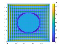
See Tables 1 and 2 for numerical results, and Fig. 3 for plots. This example aims to show that the high contrast in the diffusion coefficient results in large condition numbers, but they are still uniformly bounded, which is consistent with our main result Theorem 2.2. If we compare the degrees of freedom of and (or equivalently ) at each scale level, we observe that the former is only a fixed constant multiple of the latter for all scale levels and this constant is independent of the scale level. Table 2 demonstrates that the number of GMRES iterations required to reach the tolerance level is smaller compared to the standard FEM case and is uniformly bounded irrespective of the matrix size. This is due to fact that the wavelet coefficient matrices have small condition numbers that are uniformly bounded. On the other hand, in the case of standard FEM, the number of GMRES iterations required to reach a tolerance level of doubles with each increase in the scale level.


Example 3.2.
Consider the model problem (1.1d), where , ,
and are chosen such that the exact solution, , is
where is defined as in (3.2) for and . This makes , on , and the Dirichlet boundary condition, , nonzero on . See Table 3 for numerical results and Fig. 4 for plots.
| (ours) | (traditional) or (FEM) | ||||||||||
| order | order | order | order | ||||||||
| 4 | 2833 | 3.07E+4 | 3.85E-2 | 2.03E-1 | 225 | 5.68E-2 | 2.34E-1 | ||||
| 5 | 13589 | 4.04E+4 | 1.04E-2 | 1.68 | 1.08E-1 | 0.810 | 961 | 2.50E-2 | 1.13 | 1.26E-1 | 0.857 |
| 6 | 57317 | 4.50E+4 | 2.70E-3 | 1.87 | 5.55E-2 | 0.929 | 3969 | 1.38E-2 | 0.841 | 7.35E-2 | 0.755 |
| 7 | 233583 | 4.54E+4 | 6.88E-4 | 1.95 | 2.75E-2 | 1.00 | 16129 | 7.68E-3 | 0.833 | 4.58E-2 | 0.677 |


Example 3.3.
Consider the model problem (1.1d), where , ,
and are chosen such that the exact solution, , is
This makes on , and the Dirichlet boundary condition, , nonzero on . See Table 4 for numerical results and Fig. 5 for plots.
| (ours) | (traditional) or (FEM) | ||||||||||
| order | order | order | order | ||||||||
| 4 | 4585 | 5.33E+3 | 1.27E-1 | 3.85E-1 | 225 | 2.47E-1 | 7.19E-1 | ||||
| 5 | 22857 | 8.23E+3 | 3.01E-2 | 1.79 | 1.98E-1 | 0.828 | 961 | 1.82E-1 | 0.417 | 5.30E-1 | 0.420 |
| 6 | 97497 | 9.71E+3 | 7.79E-3 | 1.86 | 9.27E-2 | 1.05 | 3969 | 9.62E-2 | 0.900 | 3.51E-1 | 0.580 |
| 7 | 398713 | 1.08E+4 | 1.58E-3 | 2.26 | 4.71E-2 | 0.961 | 16129 | 5.24E-2 | 0.866 | 2.44E-1 | 0.519 |


Example 3.4.
Consider the model problem (1.1d), where , ,
and are chosen such that the exact solution, , is
where is defined as in (3.2) for and . This makes on , and the Dirichlet boundary condition, , nonzero on . See Table 5 for numerical results and Fig. 6 for plots.
| (ours) | (traditional) or (FEM) | ||||||||||
| order | order | order | order | ||||||||
| 4 | 3401 | 7.26E+4 | 1.19E-1 | 3.77E-1 | 225 | 6.02E-1 | 8.37E-1 | ||||
| 5 | 14361 | 9.47E+4 | 2.87E-2 | 1.96 | 1.97E-1 | 0.901 | 961 | 3.90E-1 | 0.598 | 7.10E-1 | 0.228 |
| 6 | 59361 | 1.21E+5 | 7.92E-3 | 1.82 | 1.04E-1 | 0.903 | 3969 | 2.04E-1 | 0.914 | 5.16E-1 | 0.449 |
| 7 | 241409 | 1.36E+5 | 2.08E-3 | 1.91 | 4.97E-2 | 1.04 | 16129 | 9.68E-2 | 1.06 | 3.60E-1 | 0.515 |


3.3. Examples with unknown exact solutions
We present two examples, where the exact solutions are unknown.
Example 3.5.
Consider the model problem (1.1d), where , ,
, and . The exact solution, , is unknown. See Table 6 for numerical results and Fig. 7 for plots.
| (ours) | (traditional) or (FEM) | ||||||||||
| order | order | order | order | ||||||||
| 4 | 2345 | 1.42E+2 | 24.4 | 1.49E+3 | 225 | 48.8 | 1.95E+3 | ||||
| 5 | 10401 | 1.53E+2 | 6.40 | 1.80 | 7.80E+2 | 0.865 | 961 | 26.6 | 0.836 | 1.26E+3 | 0.604 |
| 6 | 43449 | 1.65E+2 | 1.64 | 1.91 | 3.91E+2 | 0.964 | 3969 | 12.9 | 1.02 | 8.08E+2 | 0.625 |

Example 3.6.
Consider the model problem (1.1d), where and ,
, , , and , for . The exact solution, , is unknown. See Table 7 for numerical results and Fig. 8 for plots.
| (ours) | (traditional) or (FEM) | ||||||||||
| order | order | order | order | ||||||||
| 4 | 3383 | 5.86E+3 | 40.0 | 2.64E+3 | 225 | 2.16E+2 | 5.84E+3 | ||||
| 5 | 14775 | 7.63E+3 | 11.0 | 1.74 | 1.34E+3 | 0.913 | 961 | 8.53E+1 | 1.28 | 3.38E+3 | 0.756 |
| 6 | 61277 | 8.65E+3 | 3.02 | 1.82 | 6.99E+2 | 0.917 | 3969 | 5.92E+1 | 0.515 | 3.18E+3 | 0.086 |


4. Proof of Theorem 2.2
In this section, we shall prove Theorem 2.2 for the convergence rate of the Galerkin scheme using the biorthogonal wavelet on the unit interval described in Subsection 2.2.
Throughout this section, the functions and are given in (2.3) and (2.4) with their biorthogonal wavelet filter bank in (2.5) and (2.6). Then forms a biorthogonal wavelet in . It is important to notice that with , while with . Moreover, both wavelet functions and have order two vanishing moments.
To prove Theorem 2.2, we need three auxiliary results. The first auxiliary result deals with the weighted Bessel property in the fractional Sobolev space with for the wavelet system generated by the dual wavelet function and the dual refinable function in Subsection 2.2. To prove the first auxiliary result, we recall the bracket product for functions as follows:
provided that the series converges absolutely for almost every .
Using the ideas in [24, Theorem 4.6.5] and [29, Theorem 2.3], we can establish the following result.
Theorem 4.1.
Proof.
Because has compact support, we have (e.g., see [24, Lemma 4.4.1]), which is a bivariate -periodic trigonometric polynomial. Hence, , which can be also deduced from [29, Proposition 2.6] or [24, Lemma 6.3.2].
Let . We observe that
which due to Parseval’s identity yields
Since for all , we have
Hence, it follows that
where we already proved that . As a result, we have
| (4.2) |
where
We first estimate . Recall that takes the form of , , or . Thus, one of the following inequalities holds: , , or for some positive constant and for almost every . That is, for almost every . Define
Then, for all , because and , we have
which implies that . Define . Meanwhile, for , by , we have
which implies that . Continuing from (4.2), we have
where with
for all with . We obtain the desired conclusion. ∎
In preparation for the next auxiliary result, we introduce a few notations and present a few observations. Recall that . We can split the set into two groups:
| (4.3) |
Note that any must belong to either or . By construction, all elements in must have order two vanishing moments, i.e., for all . We define an integration operation along one axis as follows:
Since the tensor product part of in the -coordinate has order two vanishing moments and , we conclude that and it must have order one vanishing moment. Moreover, if , then
| (4.4) |
where . Similarly, since the tensor product part of in the -coordinate has order two vanishing moments and , we conclude that and it must have order one vanishing moment. Moreover, if , then for all , where is defined the same way as before.
To prove Theorem 2.2, we shall also need the following second auxiliary result.
Theorem 4.2.
Let with be defined in (2.10). Then there exists a positive constant such that
| (4.5) |
where is the semi-norm of in , i.e., , where and with .
Proof.
Define and . From Section 2.3, we know that is just the finite element space of the bilinear elements with the mesh size . Also, note that .
For , we define to be the interpolation function of on the grid of using the mesh size , i.e., on the grid such that for all . By [4, Theorem 4.6.14], there exists a positive constant , only depends on the hat function , such that
| (4.6) |
Note that . Because and is a biorthogonal wavelet in , by , it is critical to notice the following perpendicular condition:
| (4.7) |
We now estimate (4.5). We first handle the case, where . Integrating by parts with respect to and using the fact that satisfies the homogeneous Dirichlet condition, we obtain
Therefore, we conclude that
where we used (4.4) and the fact that to arrive at the last line. Because , we have . Note that all the elements in are compactly supported functions in and have at least one vanishing moment. Now by the Bessel property in [28, Lemma 6.1] and [22, Theorems 2.2 and 2.3], there must exist a positive constant , independent of and only depending on the wavelet, such that
| (4.8) |
We now handle the case, where . By using a similar calculation as before, we obtain
Furthermore, there exists a positive constant , independent of , such that
Combining the above estimates with (4.8), we conclude that
which combined with the approximation result in (4.6) further yields
This proves (4.5) with , where . ∎
We also need the following lemma in the proof of Theorem 2.2.
Lemma 4.3.
Let be a bounded open domain with a smooth boundary . Then
| (4.9) |
for a positive constant that only depends on but is independent of .
Proof.
For a compactly supported function , recall that its modulus of smoothness in the norm is defined by
| (4.10) |
For any , the semi-norm is
| (4.11) |
For , we define
which has a measure of order , because is a closed smooth curve. Define . Then for all , we have
for a positive constant only depending on . Consequently, we have
| (4.12) |
Note by the triangle inequality. Hence, for , we have
where we used (4.12) for the first inequality. Since and , we proved the claim with for all . ∎
We are now ready to present the proof of Theorem 2.2.
Proof of Theorem 2.2.
We split the analysis and estimation in three regions: , , and ; the last of the three is the neighborhood of the interface curve .
Proving the convergence. Because the interface is of class and by our assumption (2.16), we can extend the function from to the domain and obtain a function such that in and . Therefore, by Theorem 4.2, there exists a positive constant such that
| (4.13) |
If and is completely inside , due to on , we must have
Consequently, we conclude from (4.13) and that
| (4.14) |
where . Similarly, by assumption (2.16), in can be extended into a function such that in and . Therefore, by Theorem 4.2 and the same argument, there exists a positive constant such that for all ,
| (4.15) |
We now handle the solution in a neighborhood of the interface . Because the closed curve is completely inside , we can assume that there exist two open neighborhoods and of such that , the closure of is contained inside and the closure of is inside . Since is a curve, we can take a compactly supported smooth function supported inside such that in . Define a bivariate function . Obviously, and hence can be regarded as a function in the whole space by the zero extension outside . Therefore, applying Theorem 4.1 with and , for any , there exists a positive constant , independent of , such that
| (4.16) |
It is important to notice that is supported inside and in . Take any element
| (4.17) |
for . Because is away from the boundary and because the support of becomes smaller and smaller and closer to the interface for large enough, any element in (4.17) cannot be the boundary wavelets, i.e., we must have for some and . In addition, takes value in and the support of will be contained inside for large enough . In conclusion, there must exist a positive integer such that any element in (4.17) with must satisfy
where . Moreover, because on and , we have
for some unique , where we used the definition .
For simplicity of discussion, without loss of any generality, we can assume , because we are only interested in large for proving the convergence rate. Hence, for any satisfies (4.17) with , the above discussion implies that for and , we have
Now we conclude from the inequality (4.16) and the above estimation that
| (4.18) |
In particular, for , we have
where we used due to . Consider with . Then obviously, . Since , the above estimate can be equivalently re-expressed as follows:
| (4.19) |
In the following, we estimate the quantity for , specifically for . Define and . Then and . Moreover, and are extensions of and , respectively. Because , we consider . To estimate for , it suffices to estimate . For simplicity of discussion, we only handle and we assume that is inside and . Because , we have . Noting that , we can rewrite
because in and in . Note that and has compact support by . Consequently, there exists a positive constant such that
| (4.20) |
where only depends on the smooth function and the positive constant appeared in and . We still consider with . Then . Hence, by , we have
| (4.21) |
where holds and we used , where the positive constant only depends on and we used the inequality .
Next, we estimate . Since , by [3, Theorems C.9 and C.10] with and , there exists a positive constant only depending on such that
| (4.22) |
where the above factor is from for all in [3, Proof of Theorem C.10] by noting . Noting , we obtain from (4.9) in Lemma 4.3 that . Combining (4.20), (4.21) and (4.22), we obtain
An estimate for can be proved similarly. Note that by . Noting that and
we conclude from the above inequality estimating and similarly that
| (4.23) |
where . Since for , we deduce from (4.19) and (4.23) that , and
| (4.24) |
where , which can be written as with . Note that
where is the natural logarithm. Setting gives , i.e., because . Taking in (4.24), we conclude that , , and finally we deduce from (4.24) that
| (4.25) |
where .
Since , we have the following wavelet expansion
We define
Recall that . Then obviously,
Because is a Riesz basis of , we deduce from that there must exist a positive constant , only depending on the wavelet basis , such that
By (4.14), (4.15), and (4.25), we have
where . This proves
| (4.26) |
By the Cea’s lemma, there exists a positive constant , only depends on the diffusion coefficient and , such that
Because , we conclude that
and consequently,
| (4.27) |
where . This proves the first inequality in (2.17) for convergence in . Because , the second inequality in (2.17) follows.
Proving the convergence. We now use the Aubin-Nitsche’s technique to prove (2.18) for convergence. Note that the bilinear form is symmetric. Suppose that satisfies
| (4.28) |
and its wavelet approximated solution satisfies
By the same proof of the inequality of (4.27), we have
for some positive constant . Because and in the weak formulation (4.28), [33] (also see [12, Theorem 2.1]) guarantees the existence of a positive constant such that
where is treated as the source term for the solution in (4.28). Therefore,
| (4.29) |
Since , we deduce from that
where we used the Galerkin orthogonality for . Consequently, we deduce from (4.27) and (4.29) that
where , from which we conclude that the first inequality of (2.18) holds, i.e.,
The second inequality of (2.18) follows trivially by noting .
Proving that the condition number is uniformly bounded. Take . Then, . We want to find an upper bound for . Note that
where we used the fact that is a Riesz basis of the Sobolev space to arrive at the final inequality. Since satisfies the zero Dirichlet boundary condition, by the Poincaré inequality, we have with being a positive constant that depends only on , which implies that
Moreover, we have
where we used the fact that is a Riesz basis of the Sobolev space to arrive at the final inequality. Combining the lower and upper bounds of , we have
which gives an upper bound of the condition number in the form of , where . ∎
References
- [1] S. Adjerid, I. Babuska, R. Guo, and T. Lin, An enriched immersed finite element method for interface problems with nonhomogeneous jump conditions. Comput. Methods Appl. Mech. Engrg. 404 (2023), 115770.
- [2] I. Babuška, U. Banerjee, and K. Kergrene, Strongly stable generalized finite element method: Application to interface problems. Comput. Methods Appl. Mech. Engrg. 327 (2017), 58-92.
- [3] S. Benzoni-Gavage and D. Serre, Multidimensional hyperbolic partial differential equations. Oxford Math. Monogr. Oxford University Press, Oxford, 2007, xxvi+508 pp.
- [4] S. C. Brenner and L. R. Scott, The mathematical theory of finite element methods. Texts in Applied Mathematics. Springer, New York, 2008. xvii + 397 pp.
- [5] E. Burman and A. Ern, An unfitted hybrid high-order method for elliptic interface problems. SIAM J. Numer. Anal. 56 (2018), no. 3, 1525–1546.
- [6] E. Burman, S. Claus, P. Hansbo, M. G. Larson, and André Massing, CutFEM: Discretizing geometry and partial differential equations. Int. J. Numer. Meth. Engng. 104 (2015), 472-501.
- [7] Z. Cai, X. Ye, and S. Zhang, Discontinuous Galerkin finite element methods for interface problems: a priori and a posteriori error estimations. SIAM J. Numer. Anal. 49 (2011), no. 5, 1761-1787.
- [8] D. Černá, Wavelets on the interval and their applications, Habilitation thesis at Masaryk University, (2019).
- [9] L. Chen, H. Wei, and M. Wen, An interface-fitted mesh generator and virtual element methods for elliptic interface problems. J. Comput. Phys. 334 (2017), 327-348.
- [10] Z. Chen and Y. Liu, An arbitrarily high order unfitted finite element method for elliptic interface problems with automatic mesh generation. J. Comput. Phys. 491 (2023), 112384.
- [11] Z. Chen, K. Li, and X. Xiang, An adaptive high-order unfitted finite element method for elliptic interface problems, Numer. Math. 149 (2021), 507-548.
- [12] Z. Chen and J. Zou, Finite element methods and their convergence for elliptic and parabolic interface problems. Numer. Math. 79 (1998), 175-202.
- [13] A. Cohen, Numerical analysis of wavelet methods, Stud. Math. Appl. 32 (2003), Amsterdam.
- [14] W. Dahmen, Wavelet and multiscale methods for operator equations. Acta Numer., 6, Cambridge University Press, Cambridge, 1997, 55–228.
- [15] W. Dahmen, A. Kunoth and K. Urban, Biorthogonal spline wavelets on the interval—stability and moment conditions. Appl. Comput. Harmon. Anal. 6 (1999), 132–196.
- [16] Q. Feng, B. Han, and M. Michelle, Sixth-order compact finite difference method for 2D Helmholtz equations with singular sources and reduced pollution effect. Commun. Comput. Phys. 34 (2023), 672-712.
- [17] Q. Feng, B. Han, and P. Minev, A high order compact finite difference scheme for elliptic interface problems with discontinuous and high-contrast coefficients. Appl. Math. Comput. 431 (2022), 127314.
- [18] Q. Feng, B. Han, and P. Minev, Sixth-order hybrid finite difference methods for elliptic interface problems with mixed boundary conditions. J. Comput. Phys. 497 (2024), 112635.
- [19] H. Feng and S. Zhao, A fourth order finite difference method for solving elliptic interface problems with the FFT acceleration, J. Comput. Phys. 419 (2020), 109677.
- [20] Y. Gong, B. Li, and Z. Li, Immersed-interface finite-element methods for elliptic interface problems with nonhomogeneous jump conditions. SIAM J. Numer. Anal. 46 (2008), no. 1, 472-495.
- [21] R. Guo and T. Lin, A group of immersed finite-element spaces for elliptic interface problems. IMA J. Numer. Anal. 39 (2019), 482-511.
- [22] B. Han, Compactly supported tight wavelet frames and orthonormal wavelets of exponential decay with a general dilation matrix. J. Comput. Appl. Math. 155 (2003), 43–67.
- [23] B. Han, Nonhomogeneous wavelet systems in high dimensions. Appl. Comput. Harmon. Anal. 32 (2012), 169–196.
- [24] B. Han, Framelets and wavelets: Algorithms, analysis, and applications. Applied and Numerical Harmonic Analysis. Birkhäuser/Springer, Cham, 2017. xxxiii + 724 pp.
- [25] B. Han, Interpolating refinable functions and -step interpolatory subdivision schemes. Adv. Comput. Math. (2024), 50–98.
- [26] B. Han and M. Michelle, Derivative-orthogonal Riesz wavelets in Sobolev spaces with applications to differential equations. Appl. Comp. Harmon. Anal. 47 (2019), no. 3, 759-794.
- [27] B. Han and M. Michelle, Wavelets on intervals derived from arbitrary compactly supported biorthogonal multiwavelets. Appl. Comp. Harmon. Anal. 53 (2021), 270-331.
- [28] B. Han and M. Michelle, Wavelet Galerkin method for an electromagnetic scattering problem. https://arxiv.org/abs/2303.06770 (2023), 24 pages.
- [29] B. Han and Z. Shen, Dual wavelet frames and Riesz bases in Sobolev spaces. Constr. Approx. 29 (2009), 369-406.
- [30] A. Hansbo and P. Hansbo, An unfitted finite element method, based on Nitsche’s method, for elliptic interface problems. Comput. Methods Appl. Mech. Engrg. 191 (2002), 5537–5552.
- [31] H. Ji, F. Wang, J. Chen, and Z. Li, A new parameter free partially penalized immersed finite element and optimal convergence analysis. Numer. Math. 150 (2022), 1035-1086.
- [32] K. Kergrene, I. Babuška, and U. Banerjee, Stable generalized finite element method and associated iterative schemes; application to interface problems. Comput. Methods Appl. Mech. Engrg. 305 (2016), 1-36.
- [33] O. A. Ladyženskaja and N. N. Ural’tseva, Linear and quasilinear elliptic equations. Academic Press, New York-London, 1968, xviii+495 pp.
- [34] R. J. Leveque and Z. Li, The immersed interface method for elliptic equations with discontinuous coefficients and singular sources. SIAM J. Numer. Anal. 31 (1994), no. 4, 1019–1044.
- [35] Z. Li, T. Lin, and X. Wu, New Cartesian grid methods for interface problems using the finite element formulation. Numer. Math. 96 (2003), 61-98.
- [36] Z. Li and K. Ito, The immersed interface method: Numerical solutions of PDEs involving interfaces and irregular domains. Society for Industrial and Applied Mathematics. Philadelphia, 2006. xvi + 332 pp.
- [37] T. Lin, Y. Lin, and X. Zhang, Partially penalized immersed finite element methods for elliptic interface problems, SIAM J. Numer. Anal. 53 (2015), 1121–1144.
- [38] R. Massjung, An unfitted discontinuous Galerkin method applied to elliptic interface problems. SIAM J. Numer. Anal. 50 (2012), no. 6, 3134-3162.
- [39] B. L. Vaughan, B. G. Smith, and D. L. Chopp, A comparison of the extended finite element method with the immersed interface method for elliptic equations with discontinuous coefficients and singular sources. Comm. App. Math. and Comp. Sci. 1 (2006), no. 1, 207-228.
- [40] Q. Zhang and I. Babuška, A stable generalized finite element method (SGFEM) of degree two for interface problems. Comput. Methods Appl. Mech. Engrg. 363 (2020), 112889.
- [41] Q. Zhang, C. Cui, U. Banerjee, and I. Babuška, A condensed generalized finite element methods (CGFEM) for interface problems. Comput. Methods Appl. Mech. Engrg. 391 (2022), 114537.
- [42] Y. C. Zhou, S. Zhao, M. Feig, and G. W. Wei, High order matched interface and boundary method for elliptic equations with discontinuous coefficients and singular sources. J. Comput. Phys. 213 (2006), no. 213, 1–30.