Galactic structure dependence of cloud-cloud collisions driven star formation in the barred galaxy NGC 3627
Abstract
While cloud-cloud collisions (CCCs) have been proposed as a mechanism for triggering massive star formation, it is suggested that higher collision velocities () and lower GMC mass () or/and density () tend to suppress star formation. In this study, we choose the nearby barred galaxy NGC 3627 to examine the SFR and SFE of a colliding GMC ( and ) and explore the connections between and , () and , and galactic structures (disk, bar, and bar-end). Using ALMA CO(2–1) data (60 pc resolution), we estimated within 500 pc apertures, based on line-of-sight GMC velocities, assuming random motion in a two-dimensional plane. We extracted apertures where at least 0.1 collisions occur per 1 Myr, identifying them as regions dominated by CCC-driven star formation, and then calculated and using attenuation-corrected H data from VLT MUSE. We found that both and are lower in the bar (median values: and ), and higher in the bar-end ( and ) compared to the disk ( and ). Furthermore, we found that structural differences within the parameter space of and (), with higher () in the bar-end and higher in the bar compared to the disk, lead to higher star formation activity in the bar-end and lower activity in the bar. Our results support the scenario that variations in CCC properties across different galactic structures can explain the observed differences in SFE on a kpc scale within a disk galaxy.
1 Introduction
To understand star formation in disk galaxies, it is crucial to uncover how large-scale galactic structures (e.g., center, bar, bar-end, and arm) affect the star formation of giant molecular clouds (GMCs). Recent kpc-scale observations reveal that star formation activity varies with galactic structure (e.g., Handa et al., 1991; Momose et al., 2010; Muraoka et al., 2016; Pan & Kuno, 2017; Law et al., 2018; Yajima et al., 2019; Maeda et al., 2023). For instance, Maeda et al. (2023) found that star formation efficiency (SFE) on a kpc scale—the ratio of star formation rate (SFR) to molecular gas surface density—is statistically lower in bars and higher in centers and bar-ends compared to spiral arms. They also observed a negative correlation between SFE and CO velocity width, with low SFE and high-velocity width in bars, and high SFE and low-velocity width in bar-ends. These findings suggest that dynamical processes driven by the galactic structures significantly influence the star formation processes of GMCs, leading to variations in kpc-scale SFEs.
Several mechanisms have been proposed to explain the lower SFE in the bar region, particularly in relation to the large velocity dispersion. Bar-driven strong shocks and shear can inhibit the growth of gravitational instabilities and/or destroy GMCs, ultimately suppressing star formation (Tubbs, 1982; Athanassoula, 1992; Downes et al., 1996; Reynaud & Downes, 1998; Zurita et al., 2004; Kim et al., 2012; Meidt et al., 2013; Emsellem et al., 2015; Renaud et al., 2015; Kim et al., 2024). Observational studies further suggest that the vigorous motions in the bar region make it difficult for dense gas to survive, causing molecular gas to exist primarily as diffuse gas (e.g., Sorai et al., 2012; Muraoka et al., 2016; Maeda et al., 2020b).
This paper focuses on an alternative scenario in which galactic structures may influence the properties of cloud-cloud collisions (CCCs) themselves. CCCs are proposed as a key process that compresses molecular gas at the shock front, triggering massive star formation (e.g., Habe & Ohta, 1992; Fukui et al., 2014). Theoretical studies suggest that CCC-driven star formation may account for a few 10 to 50% of the total star formation in a disk galaxy (e.g., Tan, 2000; Kobayashi et al., 2018; Horie et al., 2024). Sub-parsec scale hydrodynamical simulations of CCCs have suggested that star formation strongly depends on the collision velocity and cloud mass (and/or density) (e.g., Takahira et al., 2014, 2018; Sakre et al., 2023). The higher the collision velocity and the lower the mass(density), the more star formation is suppressed. When the mass is fixed, faster CCCs can shorten the gas accretion phase, suppressing cloud core growth and massive star formation. At a given collision velocity, higher mass (i.e., larger size) results in a longer collision duration. Additionally, higher density increases the amount of surrounding gas available for accretion to the core. CCC observations in the Milky Way show similar dependencies (Enokiya et al., 2021; Fukui et al., 2021).
Recent observations and simulations suggest that variations in the collision velocity and mass(density) of colliding GMCs across different galactic structures may explain the observed differences in SFE on a kpc scale. Observations of GMCs in the barred galaxy NGC 1300 have reported that collision velocities may be higher in the bar region than in the arm region (Maeda et al., 2021), which may contribute to star formation suppression in the bar. Although estimated collision velocities in the bar-end are similar to those in the bar region, star formation in the bar-end region is enhanced, likely due to the larger GMC mass(density) reported in the bar-end compared to the bar (Maeda et al., 2020a). Supporting these findings, parsec-scale hydrodynamical simulations of barred galaxies indicate that GMC collision velocities in the bar region are higher than in the arm regions due to the violent gas motions driven by the bar potential (Fujimoto et al., 2014b, a, 2020) and high-density GMCs exist in the bar-end regions due to the gas inflows from both the bar and arm (Emsellem et al., 2015).
Studies of the connection between CCC velocities and galactic structures in nearby disk galaxies have been limited to NGC 1300 (Maeda et al., 2021). Focusing on the barred galaxy NGC 3627, this paper aims to quantitatively investigate the SFR and SFE of colliding GMCs, explore how GMC mass(surface density) and collision velocity are linked to galactic structures, and examine how these relationships impact the SFR and SFE of colliding GMCs. NGC 3627 is a strongly barred galaxy at a distance of 11.32 Mpc (Tully et al., 2009), with an inclination angle of (Lang et al., 2020), which is favorable for observing velocity signatures. The molecular gas surface density at the bar and bar-end regions on a kpc scale is the highest among the nearby barred galaxies (; Maeda et al., 2023), suggesting a high number density of GMCs and frequent collisions. The shock tracer CH3OH is detected in both the bar and bar-end regions (Watanabe et al., 2019, Watanabe et al. in prep), and CO(2–1) observations at a 60 pc scale by Leroy et al. (2021) reveal numerous double peak line profiles in these regions. The SFE on a kpc scale varies by about an order of magnitude between the bar and bar-end (Maeda et al., 2023), providing an opportunity to observe how differences in CCC properties contribute to variations in star formation activity across galactic structures.
Direct observations of CCCs in NGC 3627, similar to those conducted in the Milky Way (see review Fukui et al., 2021), would be ideal. However, identifying CCCs, which requires an angular resolution of a few parsecs, is challenging to achieve across the whole galaxy even with the Atacama Large Millimeter/submillimeter Array (ALMA). Therefore, using a GMC catalog identified at a 60 pc scale, we estimate the collision velocity of GMCs from their line-of-sight velocities by assuming random motion in a two-dimensional plane. In Section 2, we describe how to derive the collision velocity and SFR and SFE of a colliding GMC in detail. The data we used and the reduction process are presented in Section 3. In Section 4, we examine the SFR and SFE of colliding GMCs and explore the connections between the SFR and SFE of colliding GMCs, GMC mass(surface density) and collision velocity, and galactic structures. Section 5 investigates the uncertainties and provides interpretations of our results and comparisons with other studies. Finally, Section 6 presents a summary of this study.
2 Methodology
In an aperture (a subregion) where the star formation process is dominated by CCCs, SFR surface density can be expressed as
| (1) |
based on the CCC star formation model proposed by Tan (2000). Here is the total mass fraction of GMC gas converted to stars during a star-forming collision, is the fraction of cloud collisions that successfully lead to star formation, is the collision frequency, is the surface number density of GMCs in the aperture, and is the ensemble mean GMC mass in the aperture. A galaxy simulation by Fujimoto et al. (2014a) successfully reproduced the low SFE observed in the bar region by keeping constant and reducing for high-speed collisions. However, the and are not independent, and is not constant but varies with the collision velocity and the cloud mass/density as shown in sub-parsec simulations (Takahira et al., 2018). Since it is difficult to estimate and separately from observations, in this study we define as SFE per CCC, , and investigate the collision velocity and GMC mass/density dependence of .
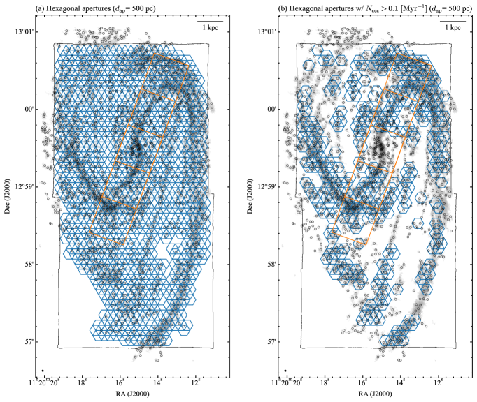
In this study, we focus on regions where the CCC-driven star formation is considered to dominate and estimate from the GMC line-of-sight velocity by assuming that the GMCs are in random motion on a two-dimensional plane within a hexagonal aperture as shown in Figure 1. Due to the random-like motion of clouds induced by the elongated gas stream in the bar potential, the determined by tracking GMCs generally agrees with those estimated under the assumption of random GMC motion in the bar and bar-end regions (Fujimoto et al., 2020; Maeda et al., 2021).
The collision velocity in the aperture is derived as
| (2) |
where is the line-of-sight velocity of the -th GMC and is the mean line-of-sight velocity within the aperture, is the number of GMCs in the aperture, and is the inclination of the disk galaxy. Then, the is derived as
| (3) |
where is the ensemble mean radius of GMCs in aperture.
Using this , we can calculate the following physical quantities within an aperture: the number of collisions that occur per unit of time (), the total mass of stars formed per CCC (), and the SFE per CCC (), given by
| (4) | |||||
| (5) | |||||
| (6) |
Since represents the molecular gas surface density in the aperture, , and corresponds to the collision timescale, , Equation (6) is equivalent to the ratio of to the molecular gas depletion time in the aperture (), i.e., .


3 Data and Reduction
3.1 Catalog of Giant Molecular Clouds
3.1.1 Data reduction for CO(2–1)
We constructed a CO(2–1) data cube at a 60 pc scale using archival data observed with the ALMA under project 2015.1.00956.S. The observations were part of the Physics at High-Angular resolution in Nearby GalaxieS (PHANGS)-ALMA project (Leroy et al., 2021), which achieved mapping of the disks of 90 nearby massive star-forming galaxies in CO(2–1) with an angular resolution of approximately . The field of view (FOV) of the NGC 3627 observations is about , covering most of the galaxy’s inner disk as shown in Figure 2(a). The observations were conducted using the 12-m, 7-m, and Total Power (TP) arrays. For both the 12 m and 7 m arrays data, we utilized calibrated visibility data provided by the East Asian ALMA Regional Center. The calibration of the TP data was performed using the Common Astronomy Software Application (CASA) package (CASA Team et al., 2022) version 4.7.0, following the script provided by the observatory.
We used CASA version 6.4.0 to reconstruct the data cube. After concatenating the visibility data sets of 12 m and 7 m arrays data, we used the tclean task with the multi-scale deconvolver (Kepley et al., 2020) for recovering extended emissions. Here, we considered scales of , , , , and . In tclean task, we applied Briggs weighting with a robust of 0.5 and used the auto-multithresh procedure to automatically identify regions containing emission in the dirty and residual images. We continued the deconvolution process until the intensity of the residual image attained the noise level. The calibrated TP data was imaged in sdimaging task.
Then, using the CASA task feather, the interferometric cube was combined with the TP cube.
The resultant angular resolution is , corresponding to , with a position angle of . The median rms noise () of the data cube is , corresponding to 132 mK in 2.5 bin. Finally, we applied the primary beam correction on the output-restored image cube.
3.1.2 GMC identification
We identified the GMCs in NGC 3627 using the PYCPROPS Python package (Rosolowsky et al., 2021). This package implements the CPROPS algorithm, originally described by Rosolowsky & Leroy (2006), and leverages the fast dendrogram algorithm provided by the ASTRODENDRO package for emission segmentation. Although the GMCs in NGC 3627 were previously identified using PYCPROPS with a CO(2–1) data cube at 90 pc resolution (Rosolowsky et al., 2021), in this study, we re-identified them at a higher resolution of 60 pc.
Below, we briefly outline the identification process and the derivation of the GMC properties. We began by identifying regions with significant emissions within the data cube. Voxels were selected where the signal exceeded 4.0 in at least two adjacent velocity channels. These voxels were then expanded to include all adjacent pixels above 2.0. Using the PYCPROPS, we decomposed the regions with significant emissions into individual GMCs. The PYCPROPS parameters for GMC identification were set to match those used in Rosolowsky et al. (2021). The process started with identifying local maxima, where the intensity () was required to be at least 2.0 higher than the merging level (). is defined as the highest value contour containing a given local maximum and one other neighboring peak. Additionally, the number of pixels above had to exceed a quarter of the beam size. Finally, the PYCPROPS assigned voxels around each local maximum to the corresponding peak using the watershed algorithm, with each local maximum being designated as an individual independent GMC.
3.1.3 Properties of GMCs
Here we summarize the properties of GMCs. The total number of GMCs is 1803, excluding those with . The distribution of the GMCs is shown in Figure 2(b). The line-of-sight velocity of a GMC, , is defined as the intensity-weighted mean velocity. PYCPROPS corrects for the sensitivity by extrapolating GMC properties to those we would expect to measure with perfect sensitivity (i.e. 0 K) and the resolution by deconvolution for the beam and channel width (see Rosolowsky & Leroy 2006 for details). The radius is defined as , where and are the extrapolated and deconvolved intensity-weighted second moments along the major and minor axis, respectively. The coefficient is set to be by assuming the surface brightness of the clouds follows a two-dimensional Gaussian (see Rosolowsky et al., 2021). Thus, the of a GMC with a size comparable to the beam size is equal to half of the geometric mean of the beam dimensions, which is 28 pc. The cumulative distribution function (CDF) of the is shown in Figure 3(a). The median in whole, bar-end, and bar are 53, 46, and 53 pc, respectively. Here, the definitions of the bar-end and bar regions follow Maeda et al. (2023), as shown in Figure 2 and described in Section 3.3.
The velocity dispersion of a GMC is defined as , where is the extrapolated velocity dispersion. The is the equivalent Gaussian width of a channel and is defined as , where is the channel width of . The median in whole, bar-end, and bar are 7.5, 9.0, and 9.5 , respectively (Figure 3(b)).
The luminosity mass of a GMC is derived as , where is the extrapolated luminosity, is a CO(1–0)-to-H2 conversion factor, and is a CO(2–1)-to-CO(1–0) brightness temperature ratio. In this study, we adopt a constant Milky Way of , including a factor of 1.36, to account for the presence of helium (Bolatto et al., 2013). We adopt based on Leroy et al. (2013) and den Brok et al. (2021), measured at kpc scales. We discuss the effect of uncertainties in the and on our results in Sections 5.1.4 and 5.1.5. The mass detection limit is estimated to be , based on the assumption that the minimum detectable GMC has a peak intensity equivalent to , a size comparable to the beam size, and a velocity width equal to twice the channel width. The median in whole, bar-end, and bar are , , and , respectively (Figure 3(c)).
The molecular gas surface density of a GMC is defined as ). The median across the whole region is 241 . As illustrated in Figures 2(a) and 3(d), the in the bar-end regions is systematically higher than that in the bar region. The median in the bar-end and bar are 557 and 308 , respectively. This difference arises because the bar-end regions tend to have systematically larger and smaller compared to the bar region (Figures 3(a) and (d)).
| Region | # | |||||||||
|---|---|---|---|---|---|---|---|---|---|---|
| () | () | () | () | () | () | () | () | (%) | ||
| All | 406 | |||||||||
| Disk | 301 | |||||||||
| Bar-end | 51 | |||||||||
| Bar | 54 |
Note. — Each physical property is noted as , where , , and are the median, the distance to the 25th percentile from the median, and the distance to the 75th percentile from the median of the number distribution, respectively.

3.2 H
As an SFR tracer, we used the H image provided by the PHANGS-MUSE project (Emsellem et al., 2022), which has the same resolution as the CO(2–1) data. The PHANGS-MUSE project provides fully calibrated data cubes and maps of 19 nearby galaxies including NGC 3627. From their data archive, we retrieved H and H maps at resolution. Note that [NII] lines around H are fitted separately and that these maps are already corrected for the Milky Way foreground extinction. The observed flux ratio of H to H is used to correct for internal extinction to the H emission. We adopted parameters in Table 2 of Calzetti (2001) for this calculation, and excluded pixels where signal-to-noise ratio (S/N) for either of the two emissions. If the calculated extinction becomes negative, no correction is applied. The median values of correction are 0.72 mag.
The is derived as
| (7) |
where is the attenuation corrected H luminosity in the aperture, and is the deprojected area of the aperture. The coefficient of is the conversion factor from H luminosity to the SFR obtained by Murphy et al. (2011). They adopted Kroupa IMF (Kroupa, 2001).
Because NGC 3627 is classified as a low-ionization nuclear emission-line region (LINER)/type 2 Seyfert galaxy (e.g., Ho et al., 1997; Filho et al., 2000), most of the H emission in the center contains contamination from the AGN. Using the BPT diagram, i.e., versus diagram, most of the H there were flagged as AGN (Emsellem et al., 2022; Groves et al., 2023). Therefore, the center region defined in Figure 2(a) is not used in this study because of the large uncertainties of the SFR.
3.3 Region mask
We adopted the definition of the center, bar, and the bar-end regions by Maeda et al. (2023). Figure 2 shows the definition as black rectangles. Maeda et al. (2023) defined a rectangle to enclose the elliptical stellar bar defined based on Spitzer 3.6 m by Herrera-Endoqui et al. (2015) and then divided the rectangle into five equal boxes. The position angle of the bar is . The length and width of the black rectangle are 8.0 and 1.5 kpc, respectively. Among the five defined boxes, the central box is referred to as the “center,” the two ends as “bar-ends,” and the boxes between them as the “bar”. The length of the rectangle was set to 1.25 times the major axis of the elliptical stellar bar to ensure that the SFR peak at the edge of the ellipse and surrounding region are included as the bar-end region. The size of the center region is approximately four times the effective radius of the bulge (Salo et al., 2015), encompassing majority of the bulge light. Notably, most of the emissions flagged as AGN in the BPT diagram (Emsellem et al., 2022; Groves et al., 2023) are located within this center region.
4 Results
4.1 Aperture setting
In this study, hexagonal apertures with a size (diameter) of were positioned to cover all the GMCs in the FoV of the H image as shown in Figure 5(a). The centers of these apertures were spaced at intervals of , representing a form of Nyquist sampling that minimizes arbitrariness in the aperture setting. The total number of apertures is 1157. The size of the aperture is roughly comparable to the width of the dust lane in the bar and arm region.
After excluding 157 apertures that contained only one GMC, we calculated the , , , and . To extract regions where the CCC-driven star formation is considered to be dominated, we then identified apertures with as regions where CCCs are considered to occur frequently. The apertures in the center region were excluded from the analysis due to the inability to estimate accurately because of the LINER activity (see Section 3.2). As a result, 406 apertures were extracted from a total of 1157 apertures. Figure 5(b) illustrates the apertures used in our analysis, showing that apertures on the bar, bar-end, and spiral arms were selected. The number of apertures in the bar-end and bar region are 51 and 54, respectively. This figure shows that regions with strong CO(2–1) emissions generally correspond to regions where CCCs are frequent in NGC 3627. The dependencies of our results on the and the aperture extraction criterion are discussed in Section 5.1.
4.2 Physical properties within the apertures
Table 1 shows the median values of the physical properties within the apertures () with in each region. The scatter is defined as the distance from the 25th percentile to the 75th percentile (the so-called “interquartile range”, IQR). In this table, “Disk” refers to the subgroup of 301 apertures other than the bar-end and bar regions. Most of the apertures classified as “disk” are located within the spiral arms, although some are in the inter-arm regions as well. Similar to Figures 3(c)-(d), the and ensemble mean GMC surface density in the aperture, , are the highest in the bar-end region. The derived from H emission in the bar-end region is about 6 times higher than that in the disk region.
Figure 5(a) shows the distribution of the collision velocity, . The median in NGC 3627 is 19.4 . We find that the in the bar region is higher, with a median of 44.4 , compared to a median of 21.0 in the bar-end region. The calculated and are also higher in the bar region compared to the bar-end region. This is primarily due to the difference in the because there is no significant difference in the between the bar and bar-end regions. The collision timescale for a GMC, , is the inverse of the , which is 27.3, 9.89, and 21.7 Myr in the disk, bar, and bar-end regions, respectively.
Figure 5(b) and (c) show the distribution of the total mass of stars formed per CCC, , and the SFE per CCC in the aperture, , respectively. In NGC 3627, the median and are and , respectively. Moreover, the median and are lower in the bar region, at and , and higher in the bar-end region, at and , compared to and in the disk region. These findings suggest that star formation activity driven by CCCs is suppressed in the bar region and enhanced in the bar-end region relative to the disk region in NGC 3627. We observe that both and decrease along the bar from the bar-end toward the center, with declining from to and decreasing from 10% to 0.01%.

4.3 Connection between star formation, collision velocity and GMC surface density/mass, and galactic structures
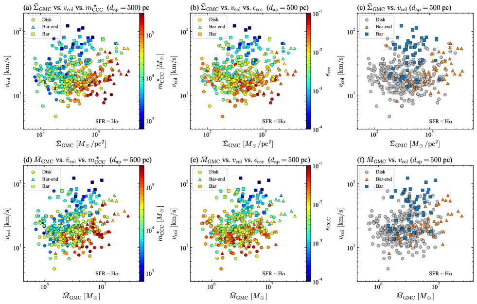
This section explores the connections between the SFR and SFE of the colliding GMC, collision velocity and GMC mass (or surface density), and galactic structures. Figure 6(a) shows the dependence of on and . The decreases with both increasing and decreasing . When exceeds and is below , generally remains under . Figure 6(b) shows dependence of on and . Similar to , the dependence of is clearly seen, while the dependence is weaker than that seen for . Note that, due to the calculation method, and inherently tend to decrease as increases. Specifically, and are calculated using Equations (3),(5) and (6), which inherently results in a tendency to be inversely proportional to .
Figure 6(c) shows the distribution of disk, bar-end, and bar apertures in the parameter space of and . When comparing the bar and bar-end regions, apertures in the bar tend to exhibit lower and higher (see also Table 1). This distribution difference leads to lower and in the bar, contrasting to higher and in the bar-end region.
Figures 6(d) and (e) are the same as panels (a) and (b) but for the dependence on and . Similar to panel (a), decreases with decreasing . However, the dependence of on at a fixed is not observed.
To clarify the structural differences within the parameter space of and (),
we performed a fitting assuming that and are proportional to a product of powers of and (). We used the curve_fit function in Python’s SciPy package, which applies non-linear least squares to fit a function to the data. Figure 7 shows the fitting results, with coefficient values provided in Table 3. As shown in Figure 6(a) and (b), both and decrease with both increasing and decreasing :
| (8) | |||
| (9) |
As shown in Figure 6(d) and (e), depends on mass, whereas is mass independent:
| (10) | |||
| (11) |
Figure 7 clearly show that the different structures have different distributions in the parameter space, with higher () in the bar-end regions and higher in the bar regions compared to the disk region, leading to differences in star-forming activity across these structures.
Once again, note that the dependence of and inherently results in a tendency to be inversely proportional to by definition. However, the fact that the best-fit power of is less than indicates that and exhibit a stronger dependence on than what is expected from the definition. This result may suggest that is physically important for suppressing star formation. Although inherently tends to be inversely proportional to , since it is calculated as (Equation (6)), dependence on does not exhibit. This is because is proportional to , which effectively cancels out the dependence of on .
5 Discussions
5.1 Uncertainties
This subsection discusses the uncertainties in our results as presented in Section 4. The results of our study under different conditions are summarized in Tables 2 and 3. While detailed analyses are provided below, our findings summarize that aperture size (Section 5.1.1) and the choice of SFR tracer (Section 5.1.3) contribute most to the uncertainties in our results. Nevertheless, our conclusions remain robust that structural differences within the parameter space of and (), with higher () in the bar-end and higher in the bar compared to the disk, lead to higher star formation activity in the bar-end and lower activity in the bar.
5.1.1 Aperture size
We varied the from 300 to 700 pc to investigate the effect of the aperture size on our results, keeping all other conditions the same. As shown in Table 2, , , , and are independent of . However, the decreases as increases, leading to a corresponding decrease in , , and , resulting in the uncertainties of about a factor of 2. This occurs because the distribution of GMCs is not uniform in the galaxy. Additionally, because the dust lane (i.e., molecular gas) width is about 500 pc (Figure 2), a larger aperture will encompass regions where CO is not detected. Although the values of and depend on the , fitting of the dependence of and on the and () are almost the same (Table 3).
5.1.2 Aperture extraction criterion
When extracting apertures, it is necessary to select regions where star formation driven by CCC is expected to be dominant. In Section 4, we imposed the condition of to include regions where, even if the is long, a high GMC number density results in frequent CCCs within the aperture. However, this criterion includes regions where is longer than the typical lifetime of a GMC of 30 Myr (e.g., Kawamura et al., 2009; Chevance et al., 2020; Kim et al., 2022; Demachi et al., 2024). Here, to more strictly extract regions where CCC-driven star formation is considered to be dominant, we select regions with smaller than 30 Myr. In this case, the number of apertures extracted is reduced by 40, 24, and 19% in the disk, bar, and bar-end regions, respectively, due to the exclusion of apertures with low . This leads to a higher mean (Table 2). Consequently, the mean and decrease by 30–40%. The fitting of the dependence of and on the and () are almost the same (Table 3).
In the case of , the extracted apertures account for of the total SFR (excluding the center region). When applying the more stringent criterion of , this fraction decreases to . These values exceed the predicted by theoretical simulations (e.g., Kobayashi et al., 2018; Horie et al., 2024). The higher fraction in NGC 3627 is reasonable since NGC 3627 has a high gas surface density and a strong bar structure, which are not considered in these predictions. Notably, the bar-end region, where CCCs are expected to be frequent, accounts for as much as of the total SFR and likely contributes to the higher fraction.
5.1.3 SFR
To check the uncertainty of the choice of star formation tracer, we use the SFR obtained from GALEX far-ultraviolet (FUV) and Spitzer 24m instead of attenuation-corrected H. The can be calculated from a linear combination of FUV and 24-m intensities by Leroy et al. (2008) as
| (12) |
where and are the FUV and 24 m intensities, respectively. The first and second terms of this equation are unobscured and embedded SFR terms, respectively. These equations assume the Kroupa IMF (Kroupa, 2001).
We used GALEX FUV and Spitzer 24-m archival data provided by Local Volume Legacy Survey (Dale et al., 2009), which are available at 10.26131/IRSA414 (catalog 10.26131/IRSA414). We used the background-subtracted FUV image with 5′′ resolution and 24-m image with 6′′ resolution. Thus, after convolving the FUV image to 6′′ resolution, the image was created following Equation (5.1.3). The is derived from the mean value of the pixels in the aperture in the image.
The values derived from H () and from FUV+24m () generally agree in regions where , with a scatter of about a factor of 2. However, in regions where , is typically about twice as large as . This difference increases as decreases. This trend, observed in many nearby galaxies (e.g., Leroy et al., 2021), is likely due to infrared cirrus components unrelated to active star formation, such as light from dust heated by older stars (e.g., Leroy et al., 2012). Consequently, in the bar region where star formation is less active, the mean is higher than .
Figure 8 is the same as Figure 6 but uses . Compared with , the dependences on and are weaker. This is because the tends to be low in regions where low-mass (or low-surface density) GMCs are present. Therefore, is higher than in these regions. Consequently, the best-fit powers of and are smaller (Table 3). Additionally, because the range of is narrower than that of , the range of and is also reduced, resulting in a shallower dependence on .

5.1.4 CO(2–1)/CO(1–0) line ratio
We assume a constant of 0.65 in calculating GMC mass based on kpc scale observations (Leroy et al., 2013; den Brok et al., 2021). However, on a kpc scale depends on galactic structures (Yajima et al., 2021; Maeda et al., 2023): The in the bar-end region tends to be higher than that in the bar region. To account for the effect of this dependence, we recalculated our results using map on a kpc scale of NGC 3627 obtained by Maeda et al. (2023). The low in the bar () and high in the bar-end () lessen the difference in GMC mass between these regions (; Table 2), thus weakening the dependence on and (Table 3). However, it is uncertain whether this correction is accurate, because the measured on a kpc scale would differ from that on a GMC scale. In the bar region of NGC 1300, in particular, on the GMC scale is reported to be higher than the kpc-scale due to diffuse molecular gas, which is distributed on scales larger than a sub-kpc and would not contribute to the star formation activity (Maeda et al., 2022). Therefore, the difference in between the bar and bar-end on a GMC scale is considered smaller than on a kpc scale. In fact, measurements at 200 pc scale in NGC 3627 show that difference in between the bar () and bar-end () is as small as (den Brok et al., 2023). This suggests that the dependences on and do not disappear. Accurate GMC mass measurements using CO(1–0) data on a GMC scale will be acquired in NGC 3627 as ALMA-FACTS project (Koda et al. in prep).
5.1.5 CO-to-H2 conversion factor
The choice of the can be the largest source of uncertainty in measuring the GMC mass. As suggested by many studies (e.g., Arimoto et al., 1996; Genzel et al., 2012; Accurso et al., 2017), the increases with the decrease in metallicity. Because the metallicity has a galactocentric radial gradient (e.g., Sánchez et al., 2014), using metallicity-dependent may change our results. The metallicity-dependent is predicted by (Accurso et al., 2017), where is the local gas phase abundance normalized to the solar value appropriate for the metallicity calibration by O3N2 method by Pettini & Pagel (2004). Using [OIII], [NII], H, and H images provided by PHANGS-MUSE projects (Emsellem et al., 2022), we calculated the metallicity in NGC 3627 and adopted the local metallicity-dependent . As a result, the mean value is nearly solar metallicity. Furthermore, the galactocentric radial variation on the is not seen in NGC 3627, which is consistent with other analysis (e.g., Kreckel et al., 2019). Consequently, our results do not change.
The can be estimated using dust, CO, and HI data under the assumption that the dust-to-gas ratio is constant at a kpc scale (Sandstrom et al., 2013), which is a method independent of the metallicity-based method described above. While the metallicity-based in NGC 3627 is not significantly different from the Milky Way , the dust-based are much lower, ranging from 0.51 to (Sandstrom et al., 2013; Yasuda et al., 2023). This suggests that the and could be 4–9 times smaller. Furthermore, unlike metallicity-based , dust-based was reported to exhibit a radial gradient, which could influence the results related to the dependences on and . The varies significantly across different studies, highlighting the need for more precise estimations as a key challenge for future research.
5.1.6 GMC identification
In this study, we use the same parameters for GMC identification with PYCPROPS as those used in the PHANGS project (Rosolowsky et al., 2021), which are considered to be the most fiducial. However, here we assess the uncertainties in GMC identification. The parameter in PYCPROPS most likely to affect results is the threshold for in local maxima identification. We apply a threshold of . Tables 2 and 3 show the results when this threshold is set to . In this case, the number of identified GMCs decreases by 43% to 1033, reducing the . However, our results do not change significantly. This stability results from applying the condition . This condition selects high-speed CCCs. Furthermore, the threshold does not affect the calculation of in regions with high-speed CCC. The threshold only determines whether two adjacent local maxima in PPV space (i.e., with similar line-of-sight velocities) are treated as a single maximum. Therefore, the threshold does not affect the calculation of in regions with high-speed CCC because the GMCs are separated in the velocity space.
Spatial resolution also affects GMC identification. However, the results remain consistent when the CO(2–1) cube is convolved to 90 pc resolution (Tables 2 and 3). The spatial resolution primarily influences the identification of spatially adjacent GMCs. Similar to the threshold of discussed above, the spatial resolution does not affect calculations when GMCs are well-separated in the velocity space.
5.2 Comparison with sub-parsec scale studies
Although and inherently tend to decrease as increases in this study (Section 2), recent sub-pc scale CCC simulations show the decreases with increasing (Takahira et al., 2014, 2018; Sakre et al., 2023).Takahira et al. (2014) and Takahira et al. (2018) conducted sub-parsec resolution simulations of CCCs between two clouds with collision speeds ranging from 3 to 30 , finding that higher collision velocities can shorten the gas accretion phase, thereby suppressing core growth and massive star formation. Consequently, the slope of the core mass function becomes steeper with increasing collision velocity, and the total mass of the cores formed decreases. Similar suppression effects are seen in magnetohydrodynamic simulations (Sakre et al., 2023).
Takahira et al. (2018) further indicates that the number of massive cores tends to increase with the mass of the colliding cloud at a fixed collision velocity, which is qualitatively consistent with our results. There are two possible reasons for this increase. First, if the radius increases with mass, the collision duration becomes longer, allowing more time for gas to accrete onto the cores. Second, if the density increases with mass, the amount of surrounding gas available for core accretion also increases. The latter effect may be significant in NGC 3627, because no correlation is seen between and within the extracted apertures.
Given the uncertainties in our results (Section 5.1), it remains unclear how depends on mass or surface density. Previous studies proposed the CCCs are responsible for the correlation between efficiency and cloud mass (e.g., Scoville et al., 1986; Ikuta & Sofue, 1997; Tan, 2000). However, in the simulation by (Takahira et al., 2018), increasing the mass or surface density tends to increase the number of high-mass cores, but it does not seem to increase .
Note that other simulations suggest star formation activity driven by CCC also depends on the angle between the magnetic field direction and the collision axis (e.g., Inoue & Inutsuka, 2009; Sakre et al., 2021). Sakre et al. (2021) found that when the two axes are nearly parallel, the converging gas flow toward the collision front is stronger, promoting the formation of massive cores. This dependence is expected to be explored in future studies of CCCs in the Milky Way.
5.3 Connection to galactic structures
Our results support the scenario that variations in the collision velocity and mass (or density) of colliding GMCs across different galactic structures may explain the observed differences in SFE on a kpc scale. The different structures have different distributions in the parameter space of and (), with higher () in the bar-end regions and higher in the bar regions compared to the disk region, leading to differences in star-forming activity across these structures.
The different distributions in the parameter space of and () by structures are interpreted as follows. The non-axisymmetric gravitational bar potential increases noncircular gas motion in the bar-end and bar region, and the crossing of cloud orbits is thought to be an environment in which molecular cloud collisions occur frequently. In the bar-end regions, gas accumulates not only because of the stagnation of the gas in the elongated elliptical orbit but also because of the inflow of the gas rotating in the disk (e.g., Downes et al., 1996), resulting in high () (e.g., Renaud et al., 2015). In the bar region, the becomes high due to the violent noncircular, streaming motions caused by the bar potential. Parsec-scale hydrodynamical simulations of barred galaxies found the collision velocity of the GMCs in the bar regions is larger than in the arm regions due to the bar potential (Fujimoto et al., 2014b, a, 2020), which is consistent with our results. Furthermore, a part of the gas that fell into the center would have overshot and sprayed into the dust lane (e.g., Sormani et al., 2019), which could be one factor contributing to the increase in the .
5.4 Comparison with previous observational studies
Previous CO observations on a kpc scale towards nearby barred galaxies showed that the velocity width in bar regions was larger than in arm and bar-end regions and that there was a negative correlation between velocity width and SFE on a kpc scale (e.g., Yajima et al., 2019; Maeda et al., 2023). This result may reflect the negative correlation between the and .
Compared to the CCC study in NGC 1300 (Maeda et al., 2021), the correlation between collision velocity, GMC mass, and star formation activity is qualitatively consistent with our findings in NGC 3627. However, NGC 3627 exhibits larger values for GMC mass, collision velocity, and collision frequency than NGC 1300. The typical values in the bar of NGC 3627 are , , and , while in the bar of NGC 1300, they are , , and . The higher collision velocity in NGC 3627 may be attributed to its stronger bar potential, as the stellar surface density derived from WISE 3.4m data (Leroy et al., 2019) is about five times higher in the bar of NGC 3627 () than that in NGC 1300 (). On a kpc scale, the gas surface density in NGC 3627 () is also one order of magnitude higher than that in NGC 1300 (), leading to significantly larger GMC mass and surface density in NGC 3627. Due to the lower GMC number density and collision velocity in NGC 1300, the collision frequency is also lower. These comparisons suggest that CCC properties may vary depending on the characteristics of the host galaxy such as morphology, stellar mass, and gas mass. Investigating the correlation between CCC properties and these factors will be an important direction for future research.
Sun et al. (2022) estimated the GMC collision timescale () for 80 PHANGS galaxies, reporting a typical value of 91 Myr—about three times longer than the 27 Myr observed in NGC 3627. Several factors could explain this discrepancy. First, since in Sun et al. (2022) was calculated across all regions with molecular gas detection, it likely includes many regions where CCC is not the dominant star formation mechanism, potentially resulting in a larger . Second, the difference could arise from the methods used to calculate the collision velocity. While our study assumes random motion, Sun et al. (2022) adopted the shear-induced collision model (Tan, 2000), which assumes CCCs occur only when clouds catch up with others in adjacent circular orbits due to orbital shear. This method may overestimate since streaming motions and intersections were not considered. Finally, NGC 3627 may be a unique disk galaxy among the 80 PHANGS galaxies, with a short collision timescale due to its high gas surface density and high GMC number density compared to other galaxies, as mentioned above. It has been suggested that a high gas surface density on a kpc scale is essential for CCC-driven star formation to dominate (e.g., Komugi et al., 2006).
6 summary
Focusing on the nearby barred galaxy NGC 3627, we quantitatively investigate the SFR and SFE of colliding GMCs, explore how GMC mass(surface density) and collision velocity are linked to galactic structures (disk, bar-end, and bar), and examine how these relationships impact the SFR and SFE of colliding GMCs. Using ALMA CO(2–1) data at a 60 pc resolution, we identified GMCs with PYCPROPS and estimated the collision velocity () in hexagonal apertures with a size of 500 pc, based on the line-of-sight velocities of GMCs and assuming random motion in a two-dimensional plane. Using the mean SFR in the apertures, derived from the attenuation-corrected H image obtained by VLT MUSE, we calculated the total mass of stars formed per CCC () and the SFE per CCC () in the apertures where CCC-driven star formation is considered to dominate (i.e., ). The main results obtained and conclusions are as follows.
-
1.
CCCs are estimated to be frequent in the bar, bar-end, and disk regions. In most of the regions with strong CO(2–1) emission, the number of collisions occurring per unit time () exceeds (Figure 5(b)).
-
2.
The median within apertures where is 19.4 . The is higher in the bar (44.4 ) compared to the bar-end (21.0 ) and disk (18.4 ) regions (Table 1). Consequently, the median is higher ( is shorter) in the bar (101.1 , 9.89 Myr) compared to the bar-end (46.1 , 21.7 Myr) and disk (36.5 , 27.3 Myr) regions.
- 3.
-
4.
The decreases with both increasing and decreasing () and the decreases with increasing (Figures 6, 7). Although these results include trends by definition, they suggest that faster CCCs shorten the gas accretion phase and low density(mass) limits the amount of gas available for accretion, thereby suppressing cloud core growth and massive star formation.
-
5.
The different structures have different distributions in the parameter space of and (), with higher () in the bar-end regions and higher in the bar regions compared to the disk region, leading to differences in star-forming activity across these structures.
-
6.
Although aperture size and the choice of SFR tracer contribute most to the uncertainties in our results, our results remain robust.
In conclusion, our results support the scenario that variations in the collision velocity and mass(density) of colliding GMCs across different galactic structures explain the observed differences in SFE on a kpc scale. However, as discussed in Section 5.4, CCC properties within galaxies may vary depending on the characteristics of the host galaxy, and more statistical surveys will be needed in the future.
| Region | # | |||||||||
|---|---|---|---|---|---|---|---|---|---|---|
| % | ||||||||||
| = 300 pc (Section 5.1.1) | ||||||||||
| All | 411 | |||||||||
| Disk | 288 | |||||||||
| Bar-end | 56 | |||||||||
| Bar | 67 | |||||||||
| = 400 pc (Section 5.1.1) | ||||||||||
| All | 423 | |||||||||
| Disk | 295 | |||||||||
| Bar-end | 62 | |||||||||
| Bar | 66 | |||||||||
| = 500 pc (Same as Table 1: Section 4) | ||||||||||
| All | 406 | |||||||||
| Disk | 301 | |||||||||
| Bar-end | 51 | |||||||||
| Bar | 54 | |||||||||
| = 600 pc (Section 5.1.1) | ||||||||||
| All | 372 | |||||||||
| Disk | 284 | |||||||||
| Bar-end | 43 | |||||||||
| Bar | 45 | |||||||||
| = 700 pc (Section 5.1.1) | ||||||||||
| All | 326 | |||||||||
| Disk | 247 | |||||||||
| Bar-end | 39 | |||||||||
| Bar | 40 | |||||||||
| (Section 5.1.2) | ||||||||||
| All | 264 | |||||||||
| Disk | 181 | |||||||||
| Bar-end | 39 | |||||||||
| Bar | 44 | |||||||||
| SFR = FUV +24m (Section 5.1.3) | ||||||||||
| All | 406 | |||||||||
| Disk | 301 | |||||||||
| Bar-end | 51 | |||||||||
| Bar | 54 | |||||||||
| variable (Section 5.1.4) | ||||||||||
| All | 406 | |||||||||
| Disk | 301 | |||||||||
| Bar-end | 51 | |||||||||
| Bar | 54 | |||||||||
| metallicity-dependent (Section 5.1.5) | ||||||||||
| All | 406 | |||||||||
| Disk | 301 | |||||||||
| Bar-end | 51 | |||||||||
| Bar | 54 | |||||||||
| (Section 5.1.6) | ||||||||||
| All | 186 | |||||||||
| Disk | 120 | |||||||||
| Bar-end | 33 | |||||||||
| Bar | 33 | |||||||||
| 90 pc resolution (Section 5.1.6) | ||||||||||
| All | 261 | |||||||||
| Disk | 195 | |||||||||
| Bar-end | 20 | |||||||||
| Bar | 46 | |||||||||
Note. — Each physical property is noted as , where , , and are the median, the distance to the 25th percentile from the median, and the distance to the 75th percentile from the median of the number distribution, respectively.
| pc | |||||||||
| pc | |||||||||
| pc | |||||||||
| pc | |||||||||
| pc | |||||||||
| SFR = FUV +24m | |||||||||
| variable | |||||||||
| metallicity-dependent | |||||||||
| 90 pc resolution | |||||||||
Note. — In the fitting of , the best-fitting coefficients are given by , , and due to the relation .
References
- Accurso et al. (2017) Accurso, G., Saintonge, A., Catinella, B., et al. 2017, MNRAS, 470, 4750, doi: 10.1093/mnras/stx1556
- Arimoto et al. (1996) Arimoto, N., Sofue, Y., & Tsujimoto, T. 1996, PASJ, 48, 275, doi: 10.1093/pasj/48.2.275
- Astropy Collaboration et al. (2018) Astropy Collaboration, Price-Whelan, A. M., Sipőcz, B. M., et al. 2018, AJ, 156, 123, doi: 10.3847/1538-3881/aabc4f
- Athanassoula (1992) Athanassoula, E. 1992, MNRAS, 259, 345, doi: 10.1093/mnras/259.2.345
- Bolatto et al. (2013) Bolatto, A. D., Wolfire, M., & Leroy, A. K. 2013, ARA&A, 51, 207, doi: 10.1146/annurev-astro-082812-140944
- Calzetti (2001) Calzetti, D. 2001, PASP, 113, 1449, doi: 10.1086/324269
- CASA Team et al. (2022) CASA Team, Bean, B., Bhatnagar, S., et al. 2022, PASP, 134, 114501, doi: 10.1088/1538-3873/ac9642
- Chevance et al. (2020) Chevance, M., Kruijssen, J. M. D., Hygate, A. P. S., et al. 2020, MNRAS, 493, 2872, doi: 10.1093/mnras/stz3525
- Dale et al. (2009) Dale, D. A., Cohen, S. A., Johnson, L. C., et al. 2009, ApJ, 703, 517, doi: 10.1088/0004-637X/703/1/517
- Demachi et al. (2024) Demachi, F., Fukui, Y., Yamada, R. I., et al. 2024, PASJ, 76, 1059, doi: 10.1093/pasj/psae071
- den Brok et al. (2021) den Brok, J. S., Chatzigiannakis, D., Bigiel, F., et al. 2021, MNRAS, 504, 3221, doi: 10.1093/mnras/stab859
- den Brok et al. (2023) den Brok, J. S., Leroy, A. K., Usero, A., et al. 2023, MNRAS, 526, 6347, doi: 10.1093/mnras/stad3091
- Downes et al. (1996) Downes, D., Reynaud, D., Solomon, P. M., & Radford, S. J. E. 1996, ApJ, 461, 186, doi: 10.1086/177046
- Emsellem et al. (2015) Emsellem, E., Renaud, F., Bournaud, F., et al. 2015, MNRAS, 446, 2468, doi: 10.1093/mnras/stu2209
- Emsellem et al. (2022) Emsellem, E., Schinnerer, E., Santoro, F., et al. 2022, A&A, 659, A191, doi: 10.1051/0004-6361/202141727
- Enokiya et al. (2021) Enokiya, R., Torii, K., & Fukui, Y. 2021, PASJ, 73, S75, doi: 10.1093/pasj/psz119
- Filho et al. (2000) Filho, M. E., Barthel, P. D., & Ho, L. C. 2000, ApJS, 129, 93, doi: 10.1086/313412
- Fujimoto et al. (2020) Fujimoto, Y., Maeda, F., Habe, A., & Ohta, K. 2020, MNRAS, 494, 2131, doi: 10.1093/mnras/staa840
- Fujimoto et al. (2014a) Fujimoto, Y., Tasker, E. J., & Habe, A. 2014a, MNRAS, 445, L65, doi: 10.1093/mnrasl/slu138
- Fujimoto et al. (2014b) Fujimoto, Y., Tasker, E. J., Wakayama, M., & Habe, A. 2014b, MNRAS, 439, 936, doi: 10.1093/mnras/stu014
- Fukui et al. (2021) Fukui, Y., Habe, A., Inoue, T., Enokiya, R., & Tachihara, K. 2021, PASJ, 73, S1, doi: 10.1093/pasj/psaa103
- Fukui et al. (2014) Fukui, Y., Ohama, A., Hanaoka, N., et al. 2014, ApJ, 780, 36, doi: 10.1088/0004-637X/780/1/36
- Genzel et al. (2012) Genzel, R., Tacconi, L. J., Combes, F., et al. 2012, ApJ, 746, 69, doi: 10.1088/0004-637X/746/1/69
- Ginsburg et al. (2019) Ginsburg, A., Sipőcz, B. M., Brasseur, C. E., et al. 2019, AJ, 157, 98, doi: 10.3847/1538-3881/aafc33
- Groves et al. (2023) Groves, B., Kreckel, K., Santoro, F., et al. 2023, MNRAS, 520, 4902, doi: 10.1093/mnras/stad114
- Habe & Ohta (1992) Habe, A., & Ohta, K. 1992, PASJ, 44, 203
- Handa et al. (1991) Handa, T., Sofue, Y., & Nakai, N. 1991, in Dynamics of Galaxies and Their Molecular Cloud Distributions, ed. F. Combes & F. Casoli, Vol. 146, 156
- Harris et al. (2020) Harris, C. R., Millman, K. J., van der Walt, S. J., et al. 2020, Nature, 585, 357, doi: 10.1038/s41586-020-2649-2
- Herrera-Endoqui et al. (2015) Herrera-Endoqui, M., Díaz-García, S., Laurikainen, E., & Salo, H. 2015, A&A, 582, A86, doi: 10.1051/0004-6361/201526047
- Ho et al. (1997) Ho, L. C., Filippenko, A. V., & Sargent, W. L. W. 1997, ApJS, 112, 315, doi: 10.1086/313041
- Horie et al. (2024) Horie, S., Okamoto, T., & Habe, A. 2024, MNRAS, 527, 10077, doi: 10.1093/mnras/stad3798
- Ikuta & Sofue (1997) Ikuta, C., & Sofue, Y. 1997, PASJ, 49, 323, doi: 10.1093/pasj/49.3.323
- Inoue & Inutsuka (2009) Inoue, T., & Inutsuka, S.-i. 2009, ApJ, 704, 161, doi: 10.1088/0004-637X/704/1/161
- Kawamura et al. (2009) Kawamura, A., Mizuno, Y., Minamidani, T., et al. 2009, ApJS, 184, 1, doi: 10.1088/0067-0049/184/1/1
- Kepley et al. (2020) Kepley, A. A., Tsutsumi, T., Brogan, C. L., et al. 2020, PASP, 132, 024505, doi: 10.1088/1538-3873/ab5e14
- Kim et al. (2022) Kim, J., Chevance, M., Kruijssen, J. M. D., et al. 2022, MNRAS, 516, 3006, doi: 10.1093/mnras/stac2339
- Kim et al. (2024) Kim, T., Gadotti, D. A., Querejeta, M., et al. 2024, ApJ, 968, 87, doi: 10.3847/1538-4357/ad410e
- Kim et al. (2012) Kim, W.-T., Seo, W.-Y., Stone, J. M., Yoon, D., & Teuben, P. J. 2012, ApJ, 747, 60, doi: 10.1088/0004-637X/747/1/60
- Kobayashi et al. (2018) Kobayashi, M. I. N., Kobayashi, H., Inutsuka, S.-i., & Fukui, Y. 2018, PASJ, 70, S59, doi: 10.1093/pasj/psy018
- Komugi et al. (2006) Komugi, S., Sofue, Y., & Egusa, F. 2006, PASJ, 58, 793, doi: 10.1093/pasj/58.5.793
- Kreckel et al. (2019) Kreckel, K., Ho, I. T., Blanc, G. A., et al. 2019, ApJ, 887, 80, doi: 10.3847/1538-4357/ab5115
- Kroupa (2001) Kroupa, P. 2001, MNRAS, 322, 231, doi: 10.1046/j.1365-8711.2001.04022.x
- Lang et al. (2020) Lang, P., Meidt, S. E., Rosolowsky, E., et al. 2020, ApJ, 897, 122, doi: 10.3847/1538-4357/ab9953
- Law et al. (2018) Law, C. J., Zhang, Q., Ricci, L., et al. 2018, ApJ, 865, 17, doi: 10.3847/1538-4357/aadca9
- Leroy et al. (2008) Leroy, A. K., Walter, F., Brinks, E., et al. 2008, AJ, 136, 2782, doi: 10.1088/0004-6256/136/6/2782
- Leroy et al. (2012) Leroy, A. K., Bigiel, F., de Blok, W. J. G., et al. 2012, AJ, 144, 3, doi: 10.1088/0004-6256/144/1/3
- Leroy et al. (2013) Leroy, A. K., Walter, F., Sandstrom, K., et al. 2013, AJ, 146, 19, doi: 10.1088/0004-6256/146/2/19
- Leroy et al. (2019) Leroy, A. K., Sandstrom, K. M., Lang, D., et al. 2019, ApJS, 244, 24, doi: 10.3847/1538-4365/ab3925
- Leroy et al. (2021) Leroy, A. K., Schinnerer, E., Hughes, A., et al. 2021, ApJS, 257, 43, doi: 10.3847/1538-4365/ac17f3
- Maeda et al. (2023) Maeda, F., Egusa, F., Ohta, K., Fujimoto, Y., & Habe, A. 2023, ApJ, 943, 7, doi: 10.3847/1538-4357/aca664
- Maeda et al. (2022) Maeda, F., Egusa, F., Ohta, K., et al. 2022, ApJ, 926, 96, doi: 10.3847/1538-4357/ac4505
- Maeda et al. (2020a) Maeda, F., Ohta, K., Fujimoto, Y., & Habe, A. 2020a, MNRAS, 493, 5045, doi: 10.1093/mnras/staa556
- Maeda et al. (2021) —. 2021, MNRAS, 502, 2238, doi: 10.1093/mnras/stab130
- Maeda et al. (2020b) Maeda, F., Ohta, K., Fujimoto, Y., Habe, A., & Ushio, K. 2020b, MNRAS, 495, 3840, doi: 10.1093/mnras/staa1296
- McMullin et al. (2007) McMullin, J. P., Waters, B., Schiebel, D., Young, W., & Golap, K. 2007, in Astronomical Society of the Pacific Conference Series, Vol. 376, Astronomical Data Analysis Software and Systems XVI, ed. R. A. Shaw, F. Hill, & D. J. Bell, 127
- Meidt et al. (2013) Meidt, S. E., Schinnerer, E., García-Burillo, S., et al. 2013, ApJ, 779, 45, doi: 10.1088/0004-637X/779/1/45
- Momose et al. (2010) Momose, R., Okumura, S. K., Koda, J., & Sawada, T. 2010, ApJ, 721, 383, doi: 10.1088/0004-637X/721/1/383
- Muraoka et al. (2016) Muraoka, K., Sorai, K., Kuno, N., et al. 2016, PASJ, 68, 89, doi: 10.1093/pasj/psw080
- Murphy et al. (2011) Murphy, E. J., Condon, J. J., Schinnerer, E., et al. 2011, ApJ, 737, 67, doi: 10.1088/0004-637X/737/2/67
- Pan & Kuno (2017) Pan, H.-A., & Kuno, N. 2017, ApJ, 839, 133, doi: 10.3847/1538-4357/aa60c2
- Pettini & Pagel (2004) Pettini, M., & Pagel, B. E. J. 2004, MNRAS, 348, L59, doi: 10.1111/j.1365-2966.2004.07591.x
- Renaud et al. (2015) Renaud, F., Bournaud, F., Emsellem, E., et al. 2015, MNRAS, 454, 3299, doi: 10.1093/mnras/stv2223
- Reynaud & Downes (1998) Reynaud, D., & Downes, D. 1998, A&A, 337, 671
- Robitaille & Bressert (2012) Robitaille, T., & Bressert, E. 2012, APLpy: Astronomical Plotting Library in Python. http://ascl.net/1208.017
- Rosolowsky & Leroy (2006) Rosolowsky, E., & Leroy, A. 2006, PASP, 118, 590, doi: 10.1086/502982
- Rosolowsky et al. (2021) Rosolowsky, E., Hughes, A., Leroy, A. K., et al. 2021, MNRAS, 502, 1218, doi: 10.1093/mnras/stab085
- Sakre et al. (2021) Sakre, N., Habe, A., Pettitt, A. R., & Okamoto, T. 2021, PASJ, 73, S385, doi: 10.1093/pasj/psaa059
- Sakre et al. (2023) Sakre, N., Habe, A., Pettitt, A. R., et al. 2023, MNRAS, 522, 4972, doi: 10.1093/mnras/stad1089
- Salo et al. (2015) Salo, H., Laurikainen, E., Laine, J., et al. 2015, ApJS, 219, 4, doi: 10.1088/0067-0049/219/1/4
- Sánchez et al. (2014) Sánchez, S. F., Rosales-Ortega, F. F., Iglesias-Páramo, J., et al. 2014, A&A, 563, A49, doi: 10.1051/0004-6361/201322343
- Sandstrom et al. (2013) Sandstrom, K. M., Leroy, A. K., Walter, F., et al. 2013, ApJ, 777, 5, doi: 10.1088/0004-637X/777/1/5
- Scoville et al. (1986) Scoville, N. Z., Sanders, D. B., & Clemens, D. P. 1986, ApJ, 310, L77, doi: 10.1086/184785
- Sorai et al. (2012) Sorai, K., Kuno, N., Nishiyama, K., et al. 2012, PASJ, 64, 51, doi: 10.1093/pasj/64.3.51
- Sormani et al. (2019) Sormani, M. C., Treß, R. G., Glover, S. C. O., et al. 2019, MNRAS, 488, 4663, doi: 10.1093/mnras/stz2054
- Sun et al. (2022) Sun, J., Leroy, A. K., Rosolowsky, E., et al. 2022, AJ, 164, 43, doi: 10.3847/1538-3881/ac74bd
- Takahira et al. (2018) Takahira, K., Shima, K., Habe, A., & Tasker, E. J. 2018, PASJ, 70, S58, doi: 10.1093/pasj/psy011
- Takahira et al. (2014) Takahira, K., Tasker, E. J., & Habe, A. 2014, ApJ, 792, 63, doi: 10.1088/0004-637X/792/1/63
- Tan (2000) Tan, J. C. 2000, ApJ, 536, 173, doi: 10.1086/308905
- Tubbs (1982) Tubbs, A. D. 1982, ApJ, 255, 458, doi: 10.1086/159846
- Tully et al. (2009) Tully, R. B., Rizzi, L., Shaya, E. J., et al. 2009, AJ, 138, 323, doi: 10.1088/0004-6256/138/2/323
- Virtanen et al. (2020) Virtanen, P., Gommers, R., Oliphant, T. E., et al. 2020, Nature Methods, 17, 261, doi: 10.1038/s41592-019-0686-2
- Watanabe et al. (2019) Watanabe, Y., Nishimura, Y., Sorai, K., et al. 2019, ApJS, 242, 26, doi: 10.3847/1538-4365/ab1d63
- Yajima et al. (2019) Yajima, Y., Sorai, K., Kuno, N., et al. 2019, PASJ, 71, S13, doi: 10.1093/pasj/psz022
- Yajima et al. (2021) Yajima, Y., Sorai, K., Miyamoto, Y., et al. 2021, PASJ, 73, 257, doi: 10.1093/pasj/psaa119
- Yasuda et al. (2023) Yasuda, A., Kuno, N., Sorai, K., et al. 2023, PASJ, 75, 743, doi: 10.1093/pasj/psad034
- Zurita et al. (2004) Zurita, A., Relaño, M., Beckman, J. E., & Knapen, J. H. 2004, A&A, 413, 73, doi: 10.1051/0004-6361:20031049