Further Evidence for the $\sim 9$ s Pulsation in LS 5039 from NuSTAR and ASCA

To quantify the PPD effect, we modify the folding analysis; below an assumed “break energy” $E_{\rm b}$, the pulse phase $\psi~{}(0\leq\psi<1)$ is linearly shifted as

where $E$ is the photon energy in keV, and $R_{\rm ppd}$ is a coefficient in units of deg keV^-1. The pulse phase at $E>E_{\rm b}$ is unchanged. A positive value of $R_{\rm ppd}$ means corrections for a “hard lag”, like in the present case, wherein a lower-energy photon is given a larger phase delay. Figure 2(b) provides an initial guess of $E_{\rm b}\sim 10$ keV, and $R_{\rm ppd}\sim 360^{\circ}$/(6 keV) =+ 60 deg keV^-1.

We first attempted to constrain $R_{\rm ppd}$. To decouple it from $E_{\rm b}$, which is likely to be above $9.4$ keV as in Figure 2(b), we chose the 3–9 keV interval and performed the epoch-folding analysis, incorporating the correction by Equation (2) in which $E_{\rm b}$ is tentatively fixed at 10.0 keV. Scanning $R_{\rm ppd}$ between $-90$ and $+90$ (1.5 times wider than the above estimate) with a step of $1.0$ (all in units of deg keV^-1), we studied how the PG peak at $P=P_{\rm NS}$ evolves. In each step of $R_{\rm ppd}$, we scanned $\tau_{0}$ from 0.723 to 0.736 (step 0.001), $a_{\rm x}\sin i$ from 47.5 to 48.5 lt-s (step 0.2), and $\omega$ from $53^{\circ}.5$ to $59^{\circ}.1$ (step $0^{\circ}.2$), but $e=0.306$ is fixed. These ranges are the same as employed in calculating Figure 1(b). The pulse period was varied over $P_{\rm NS}\pm 60~{}\mu$s, with a step of $20~{}\mu$s.

The result of this analysis is presented in Figure 3(a). Strong enhancements in $Z_{4}^{2}$ emerged at $R_{\rm ppd}\approx 62$ and $\approx-15$ deg keV^-1, with the latter somewhat higher. Compared to $Z_{4}^{2}=17.51$ at $R_{\rm ppd}=0$ (i.e., no PPD correction), the peaks at positive and negative $R_{\rm ppd}$ are higher by $\Delta Z_{4}^{2}=17.6$ and 20.2, respectively, where $\Delta Z_{4}^{2}$ means increment in $Z_{4}^{2}$; in the relevant parameter range, $\Delta Z_{4}^{2}\approx+11$ means a decrease in the chance occurrence probability by two orders of magnitude. Thus, the correction by Equation (2) appears to be working indeed, yielding two candidates of $R_{\rm ppd}$.

To estimate $E_{\rm b}$, and decide between the two $R_{\rm ppd}$ candidates, the same analysis was repeated with the energy range expanded to 3–30 keV. By testing several values of $E_{\rm b}$ from 9 keV to 11 keV, we obtained Figure 3(b). The positive-$R_{\rm ppd}$ peak, which is now at $R_{\rm ppd}=64\pm 2$ deg keV^-1, increased markedly, whereas the other candidate diminished. The mechanism working here is instructive. The PPD corrections with $R_{\rm ppd}\approx-15$ and $\approx 62$ both successfully rectified the $<10$ keV pulse phases. Compared to the 10–30 keV pulse template, the soft X-ray profile derived with $R_{\rm ppd}=64$ is in a relatively good phase alignment, but that using $R_{\rm ppd}=-15$ failed to meet this condition. As a result, the positive-$R_{\rm ppd}$ candidate grew up whereas the other became weaker, when we include the 10–30 keV photons which themselves should be insensitive to $R_{\rm ppd}$. Further considering that Figure 2(b) suggests $R_{\rm ppd}>0$, and that the value of $\tau_{0}$ (in green) associated with the positive-$R_{\rm ppd}$ peak in Figure 3(a) is closer to the Paper I result, we adopt this positive-$R_{\rm ppd}$ solution. By trimming $E_{\rm b}$ and repeating the calculation as in Figure 3(b), we obtained an estimate of $E_{\rm b}=10.4\pm 0.3$ keV.

When the PPD correction as determined above is applied to the photon arrival phases, and the orbital parameters are readjusted only slightly (Table 1), Figure 2 changed into Figure 4. In panel (a), the pulse profiles have become richer in fine structures, and they no longer drift with energy. Likewise, in panel (b), the pulse ridges run mostly straight throughout the broad energy band. The 3–10 keV pulse fraction increased to $0.042\pm 0.022$, though still much lower than in 10–30 keV (Figure 2d), and the profiles remain somewhat different from the 10-30 keV one. These are either intrinsic to the source, or due to an inaccuracy of Equation (2) in modeling the PPD effect.

To confirm the pulse recovery in soft X-rays, we created a 3–9 keV PG in Figure 5(a), incorporating the same PPD correction, and the orbital-parameter readjustment at each $P$ like in Figure 1(b). Compared to that fiducial PG, the trial period range was expanded by a factor of 13. Then, the highest significance with $Z_{4}^{2}=36.22$ is found at $P\approx 9.054$ s, whereas other peaks are all $Z_{4}^{2}<34$. As detailed in Figure 5(b), the peak is indeed right at $P_{\rm NS}$. As shown therein by an orange trace, the PPD correction also maximizes the $Z_{4}^{2}$ increment at $P_{\rm NS}$, $\Delta Z_{4}^{2}\approx 25$. Within $\sim\pm 1$ ms of $P_{\rm NS}$, this $\Delta Z_{4}^{2}$ takes systematically positive values, probably because the pulse power, once restored by the PPD correction, is partially scattered by the observing window.

Figure 5(c) shows a 3–30 keV broadband PG, produced in a similar way to (b), but using $E_{\rm b}=10.4$ keV and $R_{\rm ppd}=64$ deg keV^-1. Again at $P=P_{\rm NS}$, the PG achieves the peak with $Z_{4}^{2}=61.51$, which coincides in height with the red peak in Figure 3(b). However, the peak still remains lower than in Figure 1(b). This is because the 3–10 keV interval, where the pulse fraction is intrinsically lower, contains twice as many photons as the 10–30 keV range, and because PPD-corrected 3–10 profile (black in Figure 4a) somewhat differs from that in 10–30 keV (Figure 1d).

The 3–30 keV PG with no PPD correction, shown in black in Figure 5(c), reveals no peaks at $\sim P_{\rm NS}$, because of the dominance of soft X-ray photons. This naturally explains how the NuSTAR pulsation escaped the reconfirmation by Volkov et al. (2021), who started the timing analysis in the 3–20 keV energy interval.

When calculating Figure 5(a), we fixed $E_{\rm b}$ and $R_{\rm ppd}$ to the values optimized at $P_{\rm NS}$. Therefore, this PG is biased toward $P_{\rm NS}$, and does not correctly reflect the enlarged parameter space. However, if $R_{\rm ppd}$ is also allowed to float at each $P$, all periods examined will become equivalent, and fluctuations in $Z_{4}^{2}$ at $P\neq P_{\rm NS}$, which must be now larger, will provide a reference with which we can evaluate the statistical significance of the peak at $P=P_{\rm NS}$. (Since $E_{\rm b}=10$ keV is outside the energy range, we can fix it.) In Appendix B, we carried out this attempt, and found that the $Z_{4}^{2}$ increase in 3–9 keV at $P_{\rm NS}$, through the PPD correction (Figure 5b), has a false chance probability of ${\cal P}_{\rm ch}\sim 5\%$.

This ${\cal P}_{\rm ch}$ in 3–9 keV is rather loose, but it changes when the same evaluation is conducted in the 3–30 keV broadband. We obtain a very low chance probability of ${\cal P}_{\rm ch}\sim 0.004\%$ (Appendix B), for a value of $Z_{4}^{2}\geq 61.51$ to appear at $P_{\rm NS}$ (Figure 5c) via the PPD and orbital corrections, in which the parameters except $e$ are all readjusted at each $P$. Table 2 summarizes these results, together with those derived later from the ASCA data. Thus, the PPD effect, operating below 10 keV of the NuSTAR data, is considered real (see § 4.3).

For reference, the thin red line in Figure 5(c) is a 3–30 keV PG obtained by allowing $R_{\rm ppd}$ to float at each $P$. (The period search step of $20~{}\mu$ s is recovered here.) Thus, the effect of the enlarged parameter space is relatively limited in this energy range, typically by $\Delta Z_{4}^{2}\lesssim 10$, which is much smaller than the systematic increase at $P_{\rm NS}$, $\Delta Z_{4}^{2}\approx 42$.

Returning to the 3–9 keV interval, a support (though not quantitative) to the reality of the PPD effect is provided by Figure 6 and Table 1, where we compare the orbital constraints in 10–30 keV (Paper I) and 3–9 keV, derived without and with the PPD correction, respectively. (Here, the orbital parameters are allowed to vary over wider ranges than in Figure 5, for presentation.) The optimum values of $\omega$ (panel b) and $a_{\rm x}\sin i$ (panel a), derived in 3–9 keV using $E_{\rm b}=10$ keV and $R_{\rm ppd}=62$, are seen to depend on $\tau_{0}$ nearly in the same way as the 10–30 keV solution which is free from the PPD disturbance. The difference in $P$ by $\approx 40~{}\mu$ s is still within relative errors. Thus, the 10–30 keV photons and the PPD-corrected 3–9 keV photons, which are independent, yield nearly the same orbital constraints; they are hence thought to represent the same phenomenon.

A contrasting case is shown in Figure 6 by thin lines denoted as comparison. They represent a typical false solution in 3–9 keV, which we encountered in the calculation of Appendix B. Characterized by $P=10.5285$ s and $R=76$ deg keV^-1, it gives $Z_{4}^{2}=40.6$, and its values of $a_{\rm x}\sin i$ and $\omega$ agree with the 10–30 keV results, if evaluated at a single point of $\tau_{0}\approx 0.730$. Nevertheless, if regarded as a function of $\tau_{0}$, this false solution behaves in much different ways from the fiducial one.

Through the reanalysis of the NuSTAR data, we have thus arrived at a scenario that the object is pulsating even in energies below 10 keV, but the pulse phase suffers the PPD effect expressed by Equation (2). This result reinforces the pulse credibility (see § 4.3), and provides an important step forward in solving the issue (ii). It is also suggested that the search for pulsations in LS 5039 can be carried out using rich archival data below $\sim 10$ keV, where previous attempts were hampered presumably by the PPD perturbation which was not noticed then.

As the 1st Stage, we tentatively ignore the orbital Doppler effects, and produce $Z_{2}^{2}$ PGs over a period range of 8.2–9.2 s, which includes, and is some 14 times wider than, the range of Equation (4). The trial period is varied with a step of $\Delta P=100~{}\mu$s. We use $m=2$, because the pulse profiles would still be smeared by the orbital Doppler effects, and lack sharp features. Keeping the upper energy boundary at 12 keV, we tested four values of $E_{\rm L}$; 5.5, 6.0, 6.5, and 7.0 keV.

As in Figure 7, a promising result was derived when using the 6.0–12 keV interval; the PG reveals a clear peak, with $Z_{2}^{2}=25.1$, at a period of

which is within the tolerance of Equation (4). Since $Z_{2}^{2}$ obeys a chi-square distribution of 4 degrees of freedom, the chance probability for a value of $Z_{2}^{2}\geq 25.1$ to appear in a single trial is ${\cal P}_{\rm ch}^{(1)}=4.8\times 10^{-5}$. Given the data span of $T=63$ ks, the examined period range contains about $T/8.2-T/9.2\approx 835$ independent Fourier waves. The post-trial probability hence becomes ${\cal P}_{\rm ch}\approx 835\;{\cal P}_{\rm ch}^{(1)}\approx 4.0\%$. After multiplying this by four, the number of $E_{\rm L}$ tested, we obtain ${\cal P}_{\rm ch}=16\%$ which is given in Table 2 together with those from NuSTAR.

The above result, 16%, is relatively secure, but not constraining. As already justified, we may consider only those trials which fall in the uncertainty range of Equation (4). Then, ${{\cal P}_{\rm ch}}$ reduces to $\approx 1.2\%$ (Table 2), which is sufficiently small. Thus, $P_{0}$ is regarded as a start point of our ASCA timing analysis.

When $E_{\rm L}>6.0$ keV is used, the PG peak at $P_{0}$ diminishes, presumably because the photons would be too few. The peak also decreases when $E_{\rm L}$ is lowered from 6.0 keV, in spite of an obvious increase in the signal photon number. This suggests that the GIS data are also affected, at lower energies, by the PPD perturbation.

Although we have obtained reasonable evidence for a periodicity that is consistent with those from Suzaku and NuSTAR, we still need to perform two timing corrections before concluding on the pulse detection. One is obviously that for the orbital delays, and the other is that for the PPD effect as suggested above. The former, though well formulated, involves multiple parameters ($e,a_{\rm x}\sin i,\omega$, and $\tau_{0}$) each with residual uncertainties (Paper I). The latter, on the other hand, has only two parameters ($E_{\rm b}$ and $R_{\rm ppd}$), but the formalism is only poorly established. We also need to decide whether to conduct the two corrections simultaneously or in series, and if the latter, which should be the first.

Fortunately, the orbital phase of Equation (3) is such that the line-of-sight velocity of the source varies rather linearly with time $t$ (see § 4.1); that is, the pulse period changes with an approximately constant rate of

where $\dot{P}_{7}$ represents $\dot{P}$ in units of $10^{-7}{~{}\rm s~{}s}^{-1}$. The error includes both the uncertainty of $\tau_{0}$ in Equation (3), and the changes during the observation. We hence remove first the orbital effects approximately, by considering $\dot{P}$ in the epoch-folding procedure, in place of the full orbital corrections. The number of parameters then reduces from four to one, which is a big advantage. We also switch from $m=2$ to $m=4$ (Paper I) because fine structures will emerge in the folded pulse profiles.

As our Stage 2 attempt, we repeated the PG calculation with the GIS data, this time incorporating $\dot{P}$, to obtain $Z_{4}^{2}$ on a $(P,\dot{P})$ plane. We scanned $P$ over 8.82–8.90 s which is comparable to that of Eaquation (4), with an increment of $\Delta P=73.2~{}\mu$s, and $\dot{P}_{7}$ from 0.5 to 1.5 with an increment of $\Delta P_{7}=0.0313$. Like in Stage 1, we tested several values of $E_{\rm L}$, to compromise the signal statistics and the PPD disturbances. Then, $E_{\rm L}=5.3$ keV was found to generally maximize $Z_{4}^{2}$, rather than the 6.0 keV threshold favored in Stage 1.

The result derived from the 5.3–12 keV interval (total 859 photons) is presented in Figure 8(a). Many yellow straight lines run in parallel, with an inclination of $\approx T/2$ against the abscissa. Particularly bright are two of them, which are expressed on the plane as

They are identified in panels (b) and (c) of Figure 8, which provide two horizontal cuts across panel (a). Of these, $P_{1}$ evidently connects to the $P_{0}$ peak in Figure 7. The orbital correction is thus working at least on the $P_{1}$ branch, because it becomes highest at $\dot{P}\sim 0.7$ as expected, reaching $Z_{4}^{2}=32.1$ which exceeds the value ($Z_{4}^{2}=22.3$) at $\dot{P}=0$. The other branch, denoted as $P_{2}$, becomes higher than $P_{1}$ at $\dot{P}\sim 0.9$, whereas it gets weaker toward $\dot{P}\rightarrow 0$, connecting to a weak counterpart in the inset to Figure 7.

Below, we focus on $P_{1}$ and $P_{2}$. Either of them is actually a family of parallel lines, with a separation in $P$ by 2–15 ms. This fine structure is created presumably when an enhanced power in the data, from either the pulsation or noise fluctuations, is split by the observing window of ASCA which is a near-Earth satellite. Its data are subject to data gaps, roughly synchronized with the spacecraft’s orbital period $P_{\rm sc}\approx 5.5$ ks. Hereafter, we collectively call the family near $P_{1}$ “Solution 1” (or SOL-1), and that near $P_{2}$ “Solution 2” (or SOL-2).

Now that the orbital effect is successfully approximated by $\dot{P}$, we proceed to Stage 3, namely, incorporation of the PPD correction using Equation (2). Considering that the correction for NuSTAR worked down to the instrumental lower bound of 3.0 keV, the analysis utilizes $E_{\rm L}=2.8$ keV, which is justified later. Then, we specify a value of $\dot{P}$ in the range of Equation (6), and change $P$ over the broad interval used in Stage 1 (Figure 7) with $\Delta P=100~{}\mu$s. At each $P$, we scan $R_{\rm ppd}$ with a step of 1.0 deg keV^-1 like in the case of NuSTAR, using a wider allowance from $-180$ to $180$ deg keV^-1, and register the maximum $Z_{4}^{2}$ together with the associated $R_{\rm ppd}$. Tentatively, $E_{\rm b}$ is fixed at 10.0 keV.

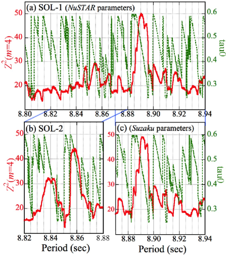
The above procedure was carried out for five values of $\dot{P}_{7}$, from 0.7 to 1.1 with a step of 0.1. The obtained five PGs are superposed in Figure 9(a). A dominant peak reaching $Z_{4}^{2}\approx 52$ has emerged at $P\approx 8.89$ s, which favors $\dot{P}_{7}=0.9$ (red). For reference, we tentatively expanded the period search range further to 7.0–11.0 s, as used in Paper I for the initial study of the NuSTAR data, but the peak at 8.89 s still remained the highest, with the next one having $Z_{4}^{2}\approx 49.1$.

In the same way as in Stage 2, the period search range is hereafter limited to 8.82–8.90 s, which accommodates the dominant peak. We re-generated PGs over this range, with a finer step of $\Delta P=20~{}\mu$s. The results are shown in panels (b), (c), and (d) of Figure 9, which employ $\dot{P}_{7}=0.9$, 0.75, and 1.05, respectively. The dominant peak in (a) is reproduced in (b) and (c), at a period of $P\approx 8.886$ s, which we hereafter denote as $P_{1}^{\prime}$. Although it differs by $\Delta P\approx 6$ ms from $P_{1}$ itself ($P_{1}=8.8791$ s for $\dot{P}_{7}=0.9$), it clearly belongs to the SOL-1 family, because we find $(1/P_{1}-1/P_{1}^{\prime})^{-1}=2.07P_{\rm sc}$ which indicates interference by the observing window. The secondary peak in (a) becomes highest in (d), and seen at $P\approx 8.855$ s $\equiv P_{2}^{\prime}$. This $P_{2}^{\prime}$ peak belongs to the SOL-2 family, because $(1/P_{2}-1/P_{2}^{\prime})^{-1}=0.84P_{\rm sc}$ holds,

Regions around the $P_{2}^{\prime}$ peak in Figure 9(d) and around the $P_{1}^{\prime}$ peak in Figure 9(b) are expanded in panels (e) and (f), respectively. There, the optimum value of $R_{\rm ppd}$ is shown in blue. Thus, $P_{1}^{\prime}$ and $P_{2}^{\prime}$ demand $R_{\rm ppd}\approx-23$ and $\approx-63$ deg keV^-1, respectively. Although the height of $P_{2}^{\prime}$ reaches a maximum of $Z_{4}^{2}=44.7$ when the involved parameters are trimmed, it remains considerably lower than that of $P_{1}^{\prime}$.

From these examinations, we regard SOL-1 as the more likely solution family, among which $P_{1}^{\prime}$ is the best pulse-period candidate under the Stage 3 formalism. The $P_{1}^{\prime}$ peak in Figure 9(f) is unlikely to be caused by statistical fluctuations, because its chance probably is sufficiently low, ${\cal P}_{\rm ch}\approx 0.2\%$ (Table 2), as evaluated in Appendix C. We hereafter concentrate on $P_{1}^{\prime}$.

The $P_{1}^{\prime}$ peak in Figure 9(f) is very sharp, because these PGs are calculated each for a fixed value of $\dot{P}$. To reflect the obvious error propagation from $\dot{P}$ to $P$, Figure 9(g) superposes the $P_{1}^{\prime}$ peaks from five values of $\dot{P}$. The composite peak is broader not only than that in Figure 9(f), but also than those in Figure 1 by several times, due to the shorter data span of ASCA.

Figure 9(g) displayed $Z_{4}^{2}$ using $P$ as an independent variable, $\dot{P}$ as a secondary parameter, and $R_{\rm ppd}$ as an implicit parameter allowed to vary over a certain range. By interchanging the roles of $P$ and $R_{\rm ppd}$ (but keeping that of $\dot{P}$), we obtain Figure 10, which is similar to Figure 3. Thus, the 2.8–12 keV GIS data constrain $R_{\rm ppd}$ very tightly. Using these results, and further trimming $E_{\rm b}$, the maximum pulse significance of $Z_{4}^{2}=53.6$ has been obtained under a condition of

together with $R_{\rm ppd}=-23.4^{+2.6}_{-3.7}$ deg keV^-1 and $E_{\rm b}=10.0^{+2.0}_{-2.3}$ keV. This $E_{\rm b}$ is very close to that found with NuSTAR, but subject to a larger error, because it is near the upper threshold of the GIS. As the largest difference from NuSTAR, $R_{\rm ppd}$ has the opposite sign.

The GIS data for the first time provide the pulse information of LS 5039 below $\sim 3$ keV. We hence varied $E_{\rm L}$ of the analysis, and found that the employed 2.8 keV gives the highest $Z_{4}^{2}$. While the $Z_{4}^{2}$ decrease toward higher $E_{\rm L}$ can be explained by a decrease of the photon number, that from $E_{\rm L}=2.8$ keV downward is not trivial. So, we tried the pulse search in 1.0–2.8 keV incorporating the orbital and PPD corrections, with $E_{\rm b}$ and $R_{\rm ppd}$ allowed to float. However, no evidence of pulsation at $\approx P_{\rm fin}$ was found ($Z_{4}^{2}<23$) in this softest interval, which contains 17% more photons than the 2.8–12 keV band. The pulse properties might change again at $\sim 2.8$ keV.

To see whether the linear energy dependence assumed in Equation (2) is appropriate, Figure 10 was recalculated for two separate energy bands, 2.8–5 keV and 5–12 keV, both using $\dot{P}_{7}=0.88$. The peak was clearly detected in both of them (though not shown), at $R_{\rm ppd}=-20^{+13}_{-14}$ ($Z_{4}^{2}=36.2$) in 2.8–5 keV, and $R_{\rm ppd}=-22\pm 6$ ($Z_{4}^{2}=22.4$) in 5–12 keV. The agreement between the two $R_{\rm ppd}$ values gives a support to Equation (2). The $Z_{4}^{2}$ peak is higher but broader in the softer band, which has twice more photons but a narrow energy span.

Thanks to the PPD correction, the periodicity found in Stage 1 and Stage 2 has thus been confirmed, with high significance, over the broad energy interval of 2.8–12 keV. Furthermore, $P_{1}^{\prime}$ is regarded as intrinsic to LS 5039, because the optimum $\dot{P}$ specified by the data, Equation (8b), approximately agrees with that predicted by the orbital Doppler effect, Equation (6).

Although our Stage 3 analysis was successful, the $\dot{P}$ approximation utilized there must be finally replaced with the proper correction for the elliptical orbit. This makes our final (4th) Stage. Hence, $\dot{P}$ is now reset to 0 as the secular spin-down rate ($\dot{P}_{7}\approx 0.0034$) is negligible. We retain $m=4$, and the 2.8–12 keV energy range together with the PPD correction, where $E_{\rm b}=10.0$ keV and $R_{\rm ppd}=-23.4$ deg keV^-1 are fixed for the moment. Then, $Z_{4}^{2}$ is calculated as a function of $P$ from 8.80 s to 8.94 s (with a step of $100\mu$s). Like in Figure 1(b) and Figure 5, at each $P$ we scan $a_{\rm x}\sin i$ from 46.5 to 53.5 lt-s (0.5 lt-s step), $\omega$ from $53^{\circ}$ to $60^{\circ}$ ($0^{\circ}.5$ step), and $\tau_{0}$ from 0.25 to 0.60 (0.002 step). The scan ranges of $a_{\rm x}\sin i$ and $\omega$ are wider than those used in § 2 (and the scan steps are coarser), to accommodate both the NuSTAR and Suzaku solutions (see Table 1). Our keen interest is whether the ASCA data favor either of the two orbital solutions, or any third one.

When $e=0.306$ from the NuSTAR solution is assumed, the PG shown in Figure 11(a) was obtained. It reveals a strong peak at

which is about 30% longer than the Suzaku plus NuSTAR prediction, but still within the uncertainty of Equation (4). As elucidated in § 4.1, the difference $P_{\rm fin}-P_{1}^{\prime}=5$ ms agrees with the Doppler shift predicted by the ephemeris of Equation (3). Furthermore, as summarized in Table 1, the derived $a_{\rm x}\sin i$ and $\omega$ agree very well with those from NuSTAR, and $\tau_{0}=0.44\pm 0.04$ is consistent with Equation (3).

We repeated the same analysis, but using $e=0.278$ (Table 1) representing the Suzaku solution. The PPD parameters were readjusted only slightly (Table  1). The obtained result, shown in Figure 11(c) and Table 1, is very similar to that in panel (a), with insignificant differences in either the peak $Z_{4}^{2}$ height or the pulse period $P_{\rm fin}$. The optimum values of $a_{\rm x}\sin i$ and $\omega$ have come to agree well with the Suzaku solution, whereas $a_{\rm x}\sin i$ now disagrees with the NuSTAR value.

As seen from the ASCA data, the two somewhat discrepant orbital solutions found with Suzaku and NuSTAR thus degenerate, and their preference cannot be decided; the issue (iii) in § 1 remains unsolved. This is because the ASCA data cover only 0.19 orbital cycles of LS 5039, whereas the Suzaku and NuSTAR data cover 1.5 and 1.0 cycles, respectively. Nevertheless, the periodicity $P_{\rm fin}$ found with ASCA satisfies a few important criteria; it is statistically significant (§ 3.2.1), it lies close to the Suzaku plus ASCA extrapolation, it is consistent with the orbital Doppler effects, and it shares the same $E_{\rm b}$ with the NuSTAR data. We hence regard $P_{\rm fin}$ as the pulse period at the ASCA observation, which is unaffected by the Suzaku vs. NuSTAR ambiguity in the orbital solution.

To complement the Stage 4 analysis, three remarks may be added. First, the peaks in Figure 11(a) and (c) are considerably broader than the composite $P_{1}^{\prime}$ peak in Figure 9(g), and by an order of magnitude than the Suzaku and NuSTAR results (Figure 1, Figure 5). This is because $P$ couples strongly with $\tau_{0}$ (dashed green trace in Figure 11a) under the very limited orbital coverage, and $\tau_{0}$ is allowed to vary beyond the interval where the $\dot{P}$ approximation works.

Next is how the orbital correction works on SOL-2. This is shown in Figure 11(b), which was obtained in the same way, but employing $E_{\rm b}=10.5$ keV and $R_{\rm ppd}=-62$ deg keV^-1. The SOL-2 peak now appears at 8.858 s, or $P_{2}^{\prime}+3$ ms, and this increment is consistent with the expected orbital effects. However, the peak, with $Z_{4}^{2}=44.3$, is still significantly lower than those in paneld (a) and (c), $Z_{4}^{2}\approx 50$. We reconfirm that $P_{\rm fin}$ of Equation (9) is the best pulse period at the barycenter of LS 5039. The SOL-2 peak may be a side lobe of $P_{\rm fin}$.

Finally, we recalculated Figure 11(a), allowing $R_{\rm ppd}$ to float at each $P$. Then, just like the relation between the blue and red traces in Figure 5(c), the baseline of $Z_{4}^{2}$ was enhanced by $\Delta Z_{4}^{2}\sim 10$, but the region around $P_{\rm fin}$ remained intact. Allowing $E_{\rm b}$ to float gave no larger effects. These results are not displayed.

In Figure 12, we compare energy-sorted pulse profiles obtained with the GIS, before (panel a) and after (panel b) the PPD correction. They are all corrected for the orbit using the parameters in Table 1, and folded at $P_{\rm fin}$ of Equation (9). In Figure 12(a), the characteristic three-peak structure is reconfirmed in the three narrow-band profiles. At the same time, we notice a clear “phase-lag” property which is reminiscent of Figure 2(a), except that the phase shift has the opposite sign. As a result, the broadband (2.8–10 keV) profile becomes rather dull. As in Figure 12(b), the PPD correction brought the narrow-band profiles into an excellent mutual phase alignment, and made them similar to one another, all clearly exhibiting the three-peak structure. The only exception is the 1–2.8 keV result, where the pulses were not confirmed (§ 3.2.3) even when applying the orbit plus PPD corrections. (The purple profile for this softest band is shown without any PPD correction.)

Table 3 summarizes how the 2.8–12 keV pulse fraction increases with the timing corrections. The values of $Z_{4}^{2}$, ${\cal P}_{\rm ch}$, and $\chi_{\rm r}$ are also given. Thus, the combined application of the orbital and PPD corrections enhances the pulse fraction, and is essential in detecting the pulsation in energies below 10 keV. However, the increase in the pulse significance is not obvious here, because the pre-trial probability ${\cal P}_{\rm ch}^{(1)}$ does not consider the trial number which evidently increases toward Case 3.

Interestingly, the final broad-band profile (in black) and the 10–30 keV profile with NuSTAR (Figure 1a) look very much alike. In Figure 12(c) we superpose them together, after appropriately scaling the GIS data (see below). The striking agreement between them strengthens that the GIS and NuSTAR data represent the same phenomenon, i.e., the source pulsation.

In Figure 12(c), the pulse-phase origin of the GIS data was shifted by $+0.15$. This is because the relative pulse phase cannot be determined uniquely between the two data sets separated by 16.9 yr s. We also rescaled the GIS counts at the $j$-th bin, $C_{j}$, into $C^{\prime}_{j}$, as

where $\bar{C}$ is the average, and the factor 4.27 is the ratio between the NuSTAR and GIS averages. The coefficient 0.54, representing “AC component”, means that the 10–30 keV pulse fraction with the NuSTAR is about half that of the 2.8–12 keV GIS data. Indeed, the 2.8–12 keV GIS pulse fraction with the full timing corrections, $0.21$ (Table 3), is 1.6 times that of the 10–30 NuSTAR profile ($0.135\pm 0.043$), although it is much lower than the 10–30 keV Suzaku result of $0.68\pm 0.14$. This pertains to the issue (iv) raised in § 1, and suggests that the pulse fraction of LS 5039 can vary significantly, in spite of the stable orbital X-ray light curves.

The profiles in Figure 12(b) use the $e=0.306$ solution in Table 1. However, even when using the $e=0.278$ solution, the profile changes little, rather than becoming similar to the 10–30 keV HXD profile in Figure 1(c). When the SOL-2 parameters (Figure 11b) are employed, the three peaks still persist, but the profile changes considerably, with the left sub peak becoming highest.

In the present work, we first reanalyzed the NuSTAR data, focusing on energies below 10 keV. We found that the 9.0538 s pulses lurk in the data even below 10 keV, but their detection is hampered by a systematic pulse-phase drift from $\approx 10$ keV down to at least 3 keV. Applying an energy-dependent correction to the timings of $\lesssim 10$ keV photons for this PPD (Pulse-Phase Drift) effect, the pulses were recovered both in 3–9 keV and in the 3–30 keV broadband, where the pulse detection was difficult before the correction. The PPD effect in the NuSTAR data is considered real, because it has ${\cal P}_{\rm ch}=0.004\%$ (§ 2.3.3, Table 2) in 3–30 keV.

The orbital solution found with the PPD-corrected signals, either in 3–9 keV or 3–30 keV, agrees with that from the hard-band (10–30 keV) NuSTAR data which are free from the PPD disturbance. Therefore, the X-ray pulses at $P_{0}$ are considered to originate from LS 5039, both above and below 10 keV.

We next analyzed the ASCA GIS data of LS 5039 in four Stages, as depicted in Figure 13 superposed on the predicted orbital Doppler curves. In Stage 1 (§ 3.2.1), a simple $m=2$ PG in 6–12 keV, covering a wide period range of $P=8.2-9.2$ s, gave evidence for periodicity at $P_{0}$ of Equation (5) (dashed green line in Figure 13). It has ${\cal P}_{\rm ch}\approx 16\%$ or $\approx 1.2\%$ (Table 2), when evaluated in the period interval of 8.2–9.2 s, or 8.82–8.90 s (consistent with Equation 4), respectively.

The Stage 2 analysis (§ 3.2.2), using the 5.3–12 keV photons, $m=4$, and the 8.82–8.90 s range, mimicked the orbital Doppler curve by a constant $\dot{P}$. Then, $Z_{4}^{2}$ increased from 25.1 (Stage 1) to 32.1, and the period was revised from $P_{0}$ to $P_{1}$ of Equation (7). The latter is shown by a magenta line, and its shift from $P_{0}$ agrees with the expected Doppler velocity difference between the mid point and the start of the observation.

In Stage 3 (§ 3.2.3), we identified the PPD effect below 10 keV with high significance (${\cal P}_{\rm ch}\approx 0.2\%$; Table 2, Appendix C), and performed its correction. The periodicity then became significant in the 2.8–12 keV broadband, when $\dot{P}_{7}\approx 0.88$ (dashed oblique line) is employed. The period changed from $P_{1}$ to $P_{1}^{\prime}$ of Equation (8a), by 6 ms which can be explained by interference with $2P_{\it sc}$. In Stage 2 and Stage 3, the approximation of the orbital effects by a constant $\dot{P}$ worked successfully.

The final (4th) step was to apply the full orbital correction to the 2.8–12 keV data, together with the PPD correction found in Stage 3. Then, the period found in Stage 1 was finally refined as $P_{\rm fin}$ of Equation (9), which falls on the zero-velocity abscissa in Figure 13. The folded profile became much more structured than with partial or no timing corrections (Table 3). This $P_{\rm fin}$, lying approximately on the NuSTAR to Suzaku back-extrapolation (§ 4.4), can be identified readily with the pulsation of LS 5039 found in Paper I. This identification is reinforced by nearly the same values of $E_{\rm b}$ between NuSTAR and ASCA, the striking similarity between the ASCA and NuSTAR pulse profiles (Figure 12c), and the consistency (Table 1) of the ASCA specified orbital parameters with those from NuSTAR  (if assuming $e=0.306$) or Suzaku  (if assuming $e=0.278$). We thus conclude that the ASCA data provide another evidence of the pulsation from LS 5039, although the issues (iii) and (iv) remain unsolved.

References

- Aragona et al. (2009) Aragona, C., McSwain, M. V., Grundstrom, E. D., et al. 2009, ApJ, 698, 514
- Araya & Harding (1999) Araya, R. A., & Harding, A. K. 1999, ApJ, 517, 334
- Bosch-Ramon (2021) Bosch-Ramon, V. 2021, A&A, 649, C1
- Brazier (1994) Brazier, K. T. 1994, MNRAS, 268, 709
- Casares et al. (2011) Casares, J., Corral-Santana, J. M., Herrero, A., et al. 2011, High-Energy Emission from Pulsars and their Systems (Berlin: Springer), 559
- Dubus (2013) Dubus, G. 2013, Astron. Ap. Review, 21, 64 (2013)
- Kishishita et. al. (2009) Kishishita, T., Tanaka, T., Uchiyama, Y., & Takahashi T. 2019, ApJ, 697, L1
- Makishima (2023) Makishima, K., 2023, Proc. IAU, 363, 267
- Makishima et al. (2014) Makishima, K., Enoto, T., Hiraga, J. S., et al. 2014, Phys. Rev. Lett., 112, 171102
- Makishima et al. (2016) Makishima, K., Enoto, T., Murakami, H., et al. 2016, PASJ, 68, S12
- Makisima et al. (2021a) Makishima, K., Enoto, T., Yoneda H., & Odaka, H. 2021b, MNRAS, 502, 2266
- Makishima et al. (1996) Makishima, K., Tashiro, M., Ebisawa, K., et al. 1996,PASJ, 48, 171
- Makisima et al. (2021b) Makishima, K., Tamba, T., Aizawa, Y., et al. 2021b, ApJ, 923, 63
- Miyasaka et al. (2013) Miyasaka, H., Bachetti M., Harrison, F. A., et al. 2013, ApJ, 775, 65
- Ohashi et al. (1996) Ohashi, T., Ebisawa, K., Fukazawa, Y., et al. 1996, PASJ, 48, 157
- Serlemitsosn et al. (1995) Serlemitsos, P. J., Jalota, L., Soong, Y., et al. 1995, PASJ, 47, 105
- Takahashi et al. (2009) Takahashi, T., Kishishita, T., Uchiyama, Y., et al. 2009, ApJ, 697, 592
- Tanaka et al. (1994) Tanaka, Y., Inoue H., & Holt, S. S. 1994, PASJ, 46, L37
- Volkov et al. (2021) Volkov, I., Kargaltsev., O, Younes, G., et al. 2021, ApJ, 615, 61
- Yoneda et al. (2023) Yoneda, H., Bosch-Ramon, V., Enoto, T., et al. 2023, ApJ, 948, 77
- Yoneda et al. (2021) Yoneda, H., Khangulyan, D, Enoto, T., et al. 2021, ApJ, 917, id.90
- Yoneda et al. (2020) Yoneda, H., Makishima, K., Enoto, T., et al. 2020, Phys. Rev. Lett., 125, id.111103 (Paper I)
- Yu et al. (2013) Yu, M., Manchester, R. N., Hobbs, G., et al. 2013, MNRAS, 429, 688