Fundamental Limit of Angular Resolution in Partly Calibrated Arrays with Position Errors
Abstract
We consider high angular resolution detection using distributed mobile platforms implemented with so-called partly calibrated arrays, where position errors between subarrays exist and the counterparts within each subarray are ideally calibrated. Since position errors between antenna arrays affect the coherent processing of measurements from these arrays, it is commonly believed that its angular resolution is influenced. A key question is whether and how much the angular resolution of partly calibrated arrays is affected by the position errors, in comparison with ideally calibrated arrays. To address this fundamental problem, we theoretically illustrate that partly calibrated arrays approximately achieve high angular resolution. Our analysis uses a special characteristic of Cramr-Rao lower bound (CRB) w.r.t. the source separation: When the source separation increases, the CRB first declines rapidly, then plateaus out, and the turning point is close to the angular resolution limit. This means that the turning point of CRB can be used to indicate angular resolution. We then theoretically analyze the declining and plateau phases of CRB, and explain that the turning point of CRB in partly calibrated arrays is close to the angular resolution limit of distributed arrays without errors, demonstrating high resolution ability. This work thus provides a theoretical guarantee for the high-resolution performance of distributed antenna arrays in mobile platforms.
Index Terms:
Partly calibrated arrays, angular resolution, the declining and plateau phases of CRB, the turning point of CRB.I Introduction
High angular resolution is desired to achieve precise target detection in applications such as radar, sonar, and astronomy. Antenna array is a common tool for direction finding. Since the angular resolution of an antenna array is inversely proportional to the aperture of the array [1], large aperture arrays are used to achieve high resolution. However, for a single array, large aperture means high system complexity, high cost and poor mobility, which restricts the scope of application.
A promising solution is to instead use multiple distributed arrays of small apertures and fuse their measurements coherently, known as ‘distributed arrays’ [2]. Ideally, distributed arrays achieve high angular resolution inversely proportional to the whole array aperture with lower system complexity. However, for distributed arrays loaded on mobile platforms such as unmanned aerial vehicles (UAVs), which are common in the low-altitude economy, drone swarms, and similar applications, it is difficult to locate the arrays accurately in real time due to the mobility of the platforms, and position errors between subarrays are unavoidable. Such distributed arrays with unknown inter-subarray position errors (and with no or calibrated intra-subarray position errors) are called partly calibrated arrays [3, 4, 5, 6, 7, 8, 9, 10, 11, 12, 13, 14]. In contrast, distributed arrays with exactly known array positions are called fully calibrated arrays [15]. A main concern is whether partly calibrated arrays could achieve the same (or similar) angular resolution as fully calibrated arrays under the negative influence of unknown errors. Note that partly calibrated arrays in this paper refer to distributed arrays with position errors between subarrays, and do not include other types of errors such as gain and phase errors [16, 17] or clock synchronization errors [18].
Though the performance of direction finding with partly calibrated arrays is intuitively inferior to the counterpart with error-free arrays, some existing algorithms experimentally show that under certain assumptions the former achieve similar angular resolution as the latter. These assumptions include, for example, high signal-to-noise rate (SNR), enough snapshots and uncorrelated source signals [4, 5], and isotropic linear arrays with the same topology [14]. However, the high-resolution ability depends on specific algorithms and their assumptions, and the scope of application is limited. Whether errors seriously degrade the resolution or not is still an open problem in more general scenarios, and is hard to solve only from the perspective of algorithm design.
Inspired by the positive empirical results, we aim to theoretically analyze the fundamental limit of angular resolution in partly calibrated arrays. The first step is to quantify angular resolution for general arrays. However, the typical Rayleigh criterion, where the central maximum of one source’s beamforming result coincides with the first minimum of the other, struggles to effectively explain the resolution of distributed arrays with errors. This is because the Rayleigh criterion is under the assumption of error-free scenarios. When errors are present, the beamforming results are significantly affected by the unknown errors and exhibit irregular behavior, making it difficult to characterize the resolution performance as in the ideal cases. This motivates us to explore alternative resolution metrics.
To this end, the statistical resolution limit (SRL) was proposed in this context and studied extensively [19, 20, 21, 22, 23, 24, 25, 26, 27]. SRL is empirically defined as the minimum separation between the parameter of interest that makes two closely spaced signals distinguishable. Several criteria are introduced to describe SRL, which are mainly divided into spectrum based [19, 20], detection based [21, 22, 23, 24] and estimation based [25, 26, 27, 28] criteria. However, the spectrum based resolution criterion is not perfectly suitable for partly calibrated arrays with position errors, since the distortion of spectral peaks caused by errors can significantly complicates the analysis. Otherwise, spectrum based and detection based criteria depend on specific estimation algorithms and hypothesis testing strategies, respectively. Estimation based criteria use estimation accuracy limit, Cramr-Rao lower bound (CRB), to characterize the resolution limit, which is independent of specific algorithms or detection strategies. However, typical CRB based criteria rely on high SNR and no modeling or signal mismatch [26], which are not directly applicable in distributed arrays with position errors. Recently, a resolution criterion based on Gaussian process was proposed [29]. However, it primarily targets optical three-dimensional imaging, making it difficult to apply directly to radar signal processing.
The main factor affecting the resolution is array aperture. To better quantify the angular resolution in a way less dependent on SNR and the error-free assumptions, we exploit a characteristic of CRB with respect to angular separation. Particularly, the CRB curve first shows a rapid decline along with the increase of the source separation from zero to a turning point. After that turning point, the curve displays minor fluctuations, and soon converges to some fixed level. The turning point is close to the angular resolution limit [26]. We explain the reason of this phenomenon as follows: 1) when sources are closely placed and are unresolvable (), the estimation accuracy is poor and the CRB is high; in this region, as the separation increases, the CRB declines, indicating the significant improvement on the estimation accuracy; when the sources becomes resolvable (), the CRB tends to be stable. This shows the rationality of using the CRB curve’s turning point as an indicator of angular resolution.
We then show that in partly calibrated arrays the CRB curve’s turning point is inversely proportional to the whole aperture of the array by analyzing the behavior of CRB in two regions: in the unresolvable part (), we show that the CRB declines polynomially with respect to and theoretically calculate the decline speed; in the resolvable part (), we illustrate that the partial derivative of CRB with respect to is close to zero. These two behaviours in the declining and plateau phases confirm the existence and location of the turning point, and consequently indicate angular resolution.
Our main contributions are summarized as follows:
-
•
We propose a new criterion that uses the turning point of CRB to indicate angular resolution;
-
•
We use the proposed criterion to demonstrate that partly calibrated arrays achieve high angular resolution similar as fully calibrated arrays, both inversely proportional to the whole array aperture.
The above conclusion provides an important theoretical guarantee for the high-resolution performance of distributed antenna arrays in mobile platforms. To our best knowledge, this work is the first to theoretically explain the high resolution performance limit of distributed arrays in the presence of position errors between subarrays.
The rest of this paper is organized as follows. Section II reviews the related works. Section III provides the signal models of fully and partly calibrated arrays. Section IV introduces our main contributions of indicating the angular resolution of partly calibrated arrays using the proposed criterion. In Section V, we detail the proofs of our main contributions. Numerical simulations are given in Section VI to verify the analysis, followed by a conclusion in Section VII.
We use , and to denote the sets of integer, real and complex numbers, respectively. The expectation of a random variable is written as . Uppercase boldface letters denote matrices (e.g. ) and lowercase boldface letters denote vectors (e.g. ). The -th element of a matrix is denoted by , and the -th column is represented by . We use to indicate the trace of a matrix and to represent a matrix with diagonal elements given by . The conjugate, transpose, and conjugate transpose operators are denoted by , respectively. The amplitude of a scalar and the norm of a vector are represented by and , respectively. The cardinality of a set is represented by . The Hadamard product is written as , the semi-definite operator is denoted by , and the definition symbol is defined as . We denote the imaginary unit for complex numbers by .
II CRB as a resolution metric
In this section, we review the related works of CRB based resolution criteria and analyze their application in indicating angular resolution of partly calibrated arrays.
To clarify the resolvability of closely spaced signals in a given scenario, SRL is an efficient typical tool that received wide attention [19, 20, 21, 22, 23, 24, 25, 26, 27, 30, 31, 32]. Particularly, SRL is defined as the minimum distance between two closely spaced signals embedded in an additive noise that allows a correct resolvability/parameter estimation [21]. One of the main techniques to describe and derive SRL is based on estimation accuracy since the resolved signals intuitively have higher estimation accuracy than the corresponding unresolved ones. CRB is widely used to characterize the upper bound of estimation accuracy, and therefore it is natural to combine SRL and CRB to explain the resolution limit.
Particularly, assume that there are two signals with frequencies mixed together and denote the resolution limit of by . Let the CRB of be written as
| (1) |
The average CRB of frequency is defined as
| (2) |
Unless otherwise emphasized, the CRBs mentioned after this section refer to the average CRB (omitting the horizontal bar).
Existing related works construct the correlation between resolution limit and CRB by some criteria. In [25], Lee criterion states that: two signals are resolvable w.r.t. the frequencies if the maximum standard deviation of each frequency estimate is less than half the difference between and , shown as . This criterion ignores the coupling between the parameters , i.e., in (1). To this end, Smith criterion in [26] states that: two signals are resolvable w.r.t. the frequencies if the difference between the frequencies, , is greater than the standard deviation of the estimation of , shown as . This means that SRL is obtained by solving the following equation,
| (3) |
where . The work in [21] extends these criteria to multidimensional harmonic retrieval cases.
However, the above metrics are only feasible in scenarios with appropriately high SNR and no modeling or signal mismatch [26]. For example, when the SNR approaches infinity, the CRB decreases to 0, implying that the resolution approaches 0 by theses criteria. This apparently contradicts the principle that the angular resolution of arrays mainly depends on the aperture, known as Rayleigh resolution limit [33]. The contradiction mainly stems from the significant influence of noise on the absolute value of CRB, and the scope of application is hence limited.
Directly using the existing CRB based criteria to analyze the angular resolution limit of partly calibrated arrays leads to impractical conclusions: We take the Smith criterion as an example. Denote the angular resolution limit of fully and partly calibrated arrays by and , respectively. Smith criterion in (3) implies that
| (4) | ||||
| (5) |
where . Since [4], we have , yielding that the angular resolution of partly calibrated arrays can be much worse than fully calibrated arrays’. This conclusion conflicts with the high-resolution performance of existing direction-finding algorithms for partly calibrated arrays [4, 5, 14].
In summary, the performance of existing CRB based criteria is seriously affected by noise and model error. The above shortcomings motivate us to propose a new resolution criterion that is less sensitive to noise and explains the angular resolution of partly calibrated arrays more practically, which is detailed in Subsection IV-A.
III Signal model
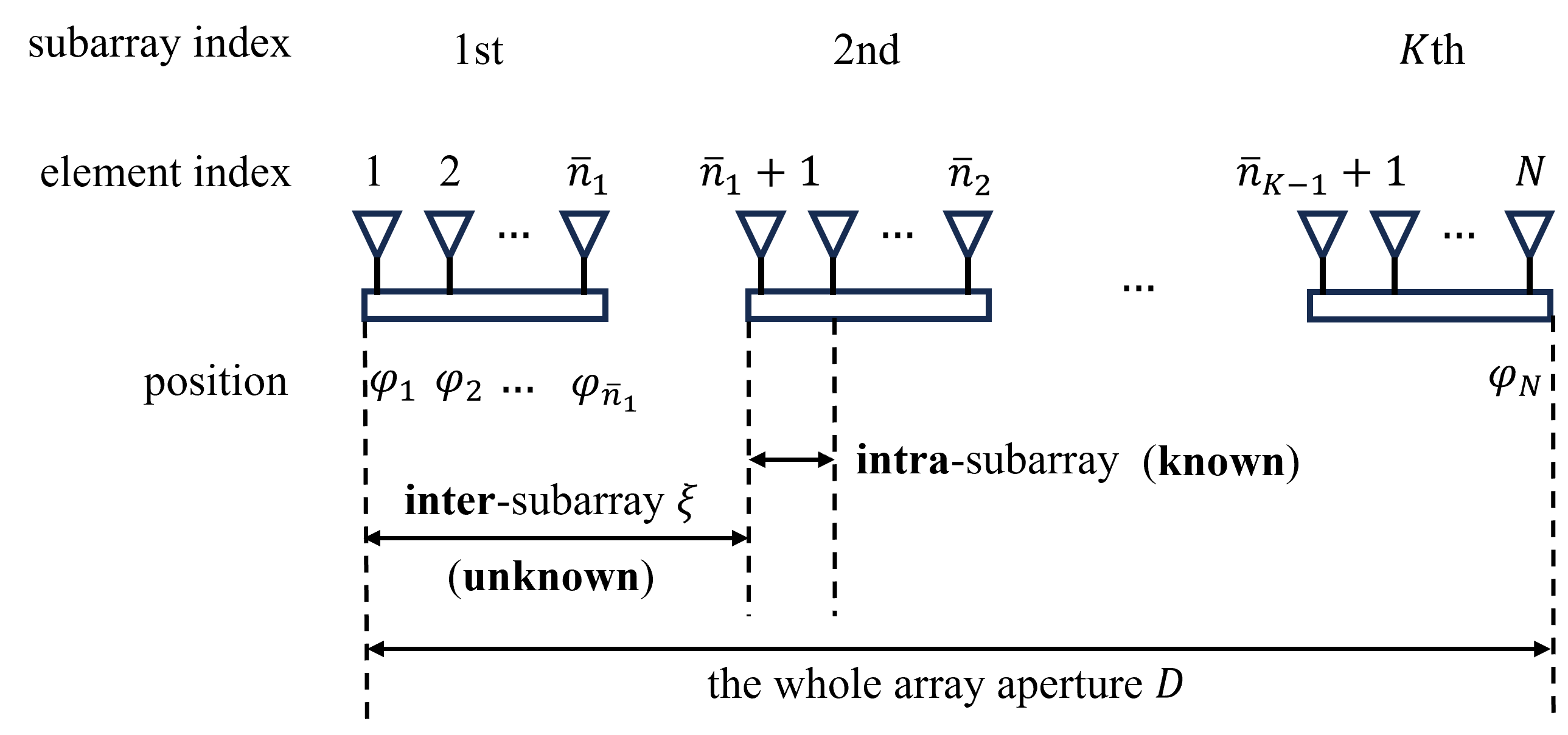
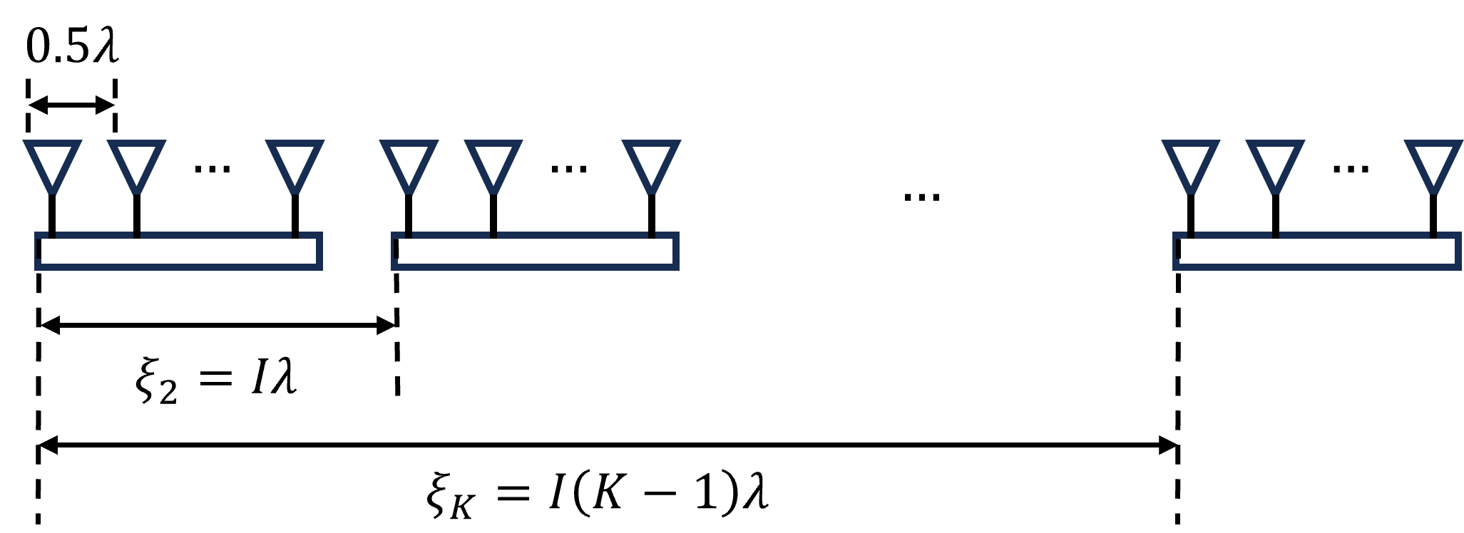
Consider linear antenna subarrays with array elements in total located on a line. The -th subarray is composed of elements, where denotes the index set of elements in the -th subarray and the full index set is denoted by . Denote by the position of the -th element relative to the 1-st element’s for . Without loss of generality, we assume , and denote the whole array aperture by . Partly calibrated arrays assume that the intra-subarray displacements, with are exactly known or well calibrated, however, the inter-subarray displacement between the -th subarray and the 1-st subarray, denoted by , is assumed unknown, where the number of elements in the first subarrays is defined as for (). In comparison, fully calibrated arrays assume that the positions of all the elements, , are exactly known. Let . Assume that the elements share a common/well-synchronized sampling clock. The diagram of partly calibrated array is shown in Fig. 1.
Consider far-field [34], narrow-band sources impinging the signals onto the whole array from different directions with . Assume that these sources are identifiable for each subarray, i.e., . Denote by the spatial angular frequency of the -th source for , where is the wavelength of the source signals. The Rayleigh resolution limit of in the fully calibrated array case is defined as (ignoring the coefficient). Denote the vectors of directions and spatial angular frequencies by and , respectively. The maximum spatial frequency separation is defined as .
In the partly calibrated array case, the received signal of the -th subarray is expressed as
| (6) |
where is the -th steering matrix, for and , contains the complex coefficients of the sources, denotes white noise with power , and denotes sample time, . Note that , where denotes the known intra-subarray displacement and denotes the unknown inter-subarray displacement.
Stacking the received signals in (6) together yields
| (7) |
where
In (7), is known, are unknown and is to be estimated. For fully and partly calibrated arrays, in is assumed to be completely known and unknown, respectively. For conciseness, we abbreviate to , to and to , respectively.
The CRBs of spatial frequencies in fully and partly calibrated arrays, denoted by and , respectively, are shown in Appendix A.
IV Our main contributions
In this section, we detail our main contributions: 1) propose a new CRB based resolution criterion less sensitive to noise and model error; 2) use the proposed criterion to show that partly calibrated arrays achieve high angular resolution similar to fully calibrated arrays.
Particularly, we first introduce the intuition behind the proposed criterion of indicating angular resolution by the turning point of CRB in Subsection IV-A. We then analyze the angular resolution of partly calibrated arrays and show the high-resolution ability in Subsection IV-B. Finally, we apply the proposed resolution criterion to fully calibrated arrays and compare the analysis results with prior works in Subsection IV-C.
IV-A The proposed resolution criterion
To meet the challenge of analyzing the resolution limit of partly calibrated arrays, we propose a new resolution criterion using the turning point of CRB. The proposed criterion states that: two signals are said to be resolvable w.r.t. the frequencies if the difference between the frequencies, , is greater than the turning point of CRB w.r.t. denoted by . The definition of the CRB turning point is detailed in Section V-D.
The basic principle of this criterion is based on a significant phenomenon of : Fix the source of as a reference and gradually increase the frequency difference . The first declines rapidly w.r.t. , and then it almost remains constant (with a small fluctuation). The turning point is located close to the angular resolution limit. We show this phenomenon in fully and partly calibrated arrays as an example. Consider using half-wavelength, uniform linear subarrays to estimate the directions of sources with the angles , where denotes the angle difference. There are elements in each subarray and the adjacent subarrays are spaced at half-wavelength apart. Denote by the angular resolution limit, where is the whole array aperture. The CRBs of fully and partly calibrated arrays, and , are shown in Fig. 2.
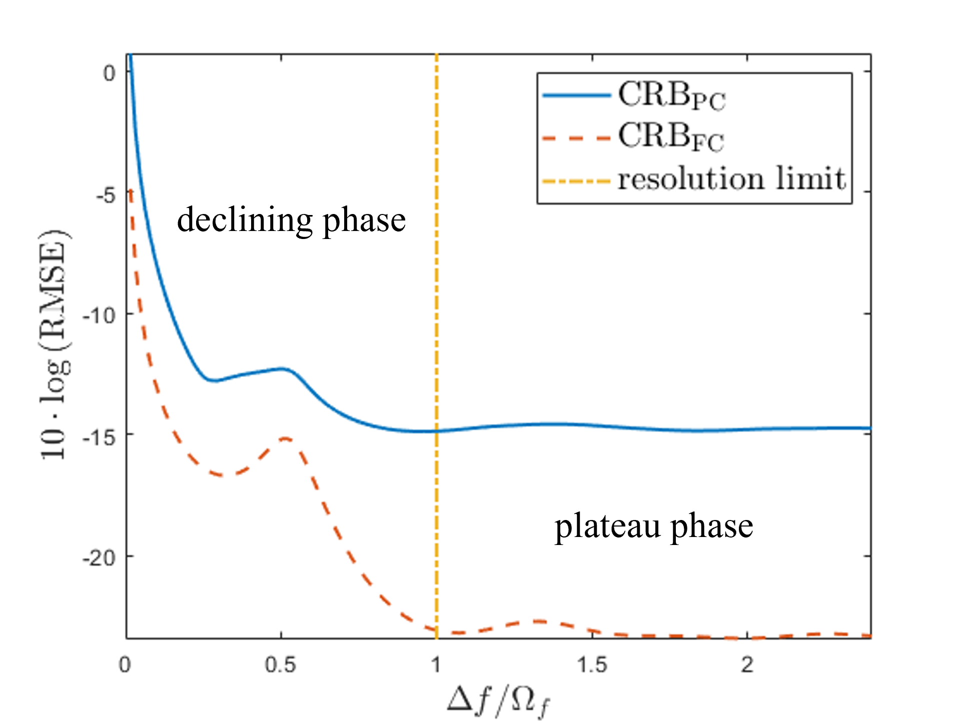
From Fig. 2, we find that the two CRBs decline when , and tend to be stable when . We provide an intuitive explanation of this phenomenon: when the frequency difference is within the resolution limit , the sources cannot be distinguished, disrupting the estimation performance and greatly increasing the CRB; in this case, increasing increases the resolvability and hence decreases the CRB, which corresponds to the declining phase of the CRB. When exceeds , the estimation accuracy is close to the counterpart of estimating the sources separately [25]; consequently, the accuracy is less relevant to , keeping the CRB constant, which corresponds to the plateau phase of the CRB. Here, ’plateaus phase’ refers to a situation where, after some change, a trend or curve stabilizes and no longer shows significant variation or fluctuation, which is consistent with the CRB when . Therefore, the turning point between the declining and the plateau phases indicates angular resolution.
For another reason, we use the turning point of CRB as the angular resolution limit since it can reflect the influence on each other for parameter estimation, which is precisely the meaning of resolution. Particularly, when two sources are not distinguished, they significantly influence each other, resulting in poor estimation performance as reflected in the decline part of CRB. When the two sources can be separated, their mutual influence is minimal, and the CRB approaches the performance of separate estimation. Thus, the transition point between these two states can be used to indicate the resolution, which is the turning point of CRB.
The reason that the turning point is not exactly located at is that on one hand, the theoretical proof in the paper represents the result in a statistical average sense (see the A2 assumption in Section V), which cannot ensure that the turning point of the CRB in every specific scenario precisely locates on the resolution cell; on the other hand, resolution criterion, either the Rayleigh resolution limit or 3dB beam width, is an empirical concept, which is not an absolute indication of separability or non-separability. Overall, it can ensure that the magnitude of the resolution is correct.
In the proposed resolution criterion, angular resolution depends not only on the angular difference but also on the absolute angle values. This is because that we use the frequency separation, , to reflect source separation instead of angle separation, . Particularly in Fig. 2, we have and . Through trigonometric transformation, we have
| (8) |
In the above equation, the sin part reflects the angular resolution and the cos part reflects the angle values themselves. Therefore, the CRB is not only related to the angle separation , but also angle values . It can be found that large angle values have worse resolution.
Note that the proposed resolution criterion using the CRB turning point is almost unaffected by SNR. This is because in the CRB expression (see (35) and (36) in Appendix A), the component of white noise can be isolated, which means that it only affects the absolute value of the CRB without altering its relative variation with respect to the angle difference. Although this property contradicts the commonly held conclusion that resolution is related to SNR, it is rational in analyzing the effect of position errors in distributed arrays. This is because that inter-subarray position errors fundamentally differ from white noise errors: the former are multiplicative errors, while the latter are additive errors. When the SNR is extremely low, it becomes impossible to distinguish and estimate the angles, making it ineffective to analyze the impact of multiplicative errors on resolution. Therefore, we aim to conduct an analysis method that is unaffected or minimally affected by additive noise. The proposed resolution criterion using the CRB turning point can effectively address this challenge.
In the sequel, we apply the proposed criterion to analyze the angular resolution of fully and partly calibrated arrays. A main conclusion is that partly calibrated arrays achieve high resolution similar to that of fully calibrated arrays. Note that the above phenomenon of CRB w.r.t. was also mentioned in previous works [25, 26], but they did not use it to indicate resolution and provide the corresponding theoretical guarantees. The key challenge is to analyze the partial derivative of CRB to , which is hard to analytically calculate. In Section V, we provide an approximate method to solve this problem.
IV-B Resolution analysis on partly calibrated arrays
Here, we analyze the declining phase, plateau phase, and turning point of , and use the turning point to indicate angular resolution of partly calibrated arrays.
IV-B1 Declining phase of
We analyze the declining phase of using small quantity approximation, shown as Proposition 1, which illustrates that the main declining rate of is proportional to .
Proposition 1 (declining phase for partly calibrated arrays).
When , we have
| (9) |
where is a constant w.r.t. .
Proof.
See Appendix B. ∎
IV-B2 Plateau phase of
We analyze the plateau phase of , shown as Proposition 2, where the assumptions are detailed in Subsection V-A. Proposition 2 illustrates that remains almost constant w.r.t. when . Here denotes the functional relationship between CRB and instead of the CRB of .
Proposition 2 (plateau phase for partly calibrated arrays).
Under assumptions A1-A3, when , we have
| (10) |
with high probability.
Proof.
See Subsection V-B. ∎
This proposition illustrates that under the scenario of using a large, sparse, uniformly distributed array to resolve two closely spaced sources (corresponding to assumptions A1-A3 in Section V-A), remains almost constant w.r.t. when . Based on the proposed criterion, the stable CRB implies that the sources are resolvable in this situation. The approximation in Proposition 2 is used for the convenience of explanation and a more rigorous expression is detailed in the corresponding proof.
IV-B3 Turning point of
Intuitively, the intersection of the declining phase and plateau phase of CRB corresponds to the turning point. Based on Proposition 1 and Proposition 2, a criterion [35] is used to determine the turning point of in a strict sense, given by
| (11) |
where the explanation is detailed in Subsection V-D.
The conclusion of applying our proposed resolution criterion to in (11) implies that high angular resolution is achievable for partly calibrated arrays, inversely proportional to the whole array aperture , which is consistent with existing direction-finding algorithms for partly calibrated arrays [4, 5, 14]. A main advantage relative to the existing CRB based SRL criteria is that the proposed criterion is less sensitive to noise. This helps to focus on the main factors that affect the resolution (array aperture), while reducing the interference of secondary factors (noise), and avoid the limitations of existing CRB based criteria.
IV-C Resolution analysis on fully calibrated arrays
For comparison, we analyze the declining phase, plateau phase, and turning point of , and use the turning point to indicate angular resolution of fully calibrated arrays.
IV-C1 Declining phase of
The declining phase of has been theoretically analyzed using small quantity approximation in [25], shown as Lemma 1. It is proven that when , declines at the rate mainly proportional to , which is the same as the counterpart of .
Lemma 1 (declining phase for fully calibrated arrays[25]).
When , we have
| (12) |
where is a constant w.r.t. .
IV-C2 Plateau phase of
We analyze the plateau phase of in Proposition 3, which illustrates that remains almost constant w.r.t. when . The rigorous expression is similar to the counterpart of , which is detailed in the corresponding proof.
Proposition 3 (plateau phase for fully calibrated arrays).
Under assumptions A1-A3, when , we have
| (13) |
with high probability.
Proof.
See Subsection V-C. ∎
IV-C3 Turning point of
Based on Lemma 1 and Proposition 3, we use the criterion in [35] to determine the turning point of in a strict sense, given by
| (14) |
where the explanation is similar with that of .
Based on the proposed criterion, (14) means that the resolution limit of fully calibrated arrays is inversely proportional to the whole array aperture , which is consistent with existing Rayleigh resolution limit. This verifies the feasibility of the proposed criterion and supports to apply it on the resolution analysis of partly calibrated arrays.
Our main contributions on theoretically analyzing the declining phase, plateau phase and turning point of CRB are summarized in Table I.
| fully calibrated | partly calibrated | |
| declining phase | Lemma 1 [25] | Proposition 1 |
| plateau phase | Proposition 3 | Proposition 2 |
| turning point |
Note that the super-resolution phenomenon in the existing self-calibration methods does not contradict the conclusion of this paper. This is because existing super-resolution algorithms [36, 37] make additional prior assumptions about the scenario and model, whereas the signal model in this paper does not. For instance, sparse recovery algorithms assume that targets are sparsely located within the solution space, and subspace methods assume uncorrelated source signals. These assumptions introduce extra feature information compared to the classical model, thereby affecting the model’s performance bounds, which manifest as improvements in resolution. However, we base our study on the classical model assumptions without incorporating other prior assumptions such as sparsity, and therefore, it does not involve super-resolution performance.
V Proof of the propositions in Section IV
In this section, we prove Propositions 2 and 3, while the proof of Proposition 1 is left to Appendix B since it is a direct extension of [25]. First, we introduce assumptions A1-A3 in Subsection V-A, followed by the detailed proofs of Propositions 2 and 3 in Subsection V-B and V-C, respectively. Based on the proofs above, we explain how to determine the turning point of CRB in Subsection V-D.
V-A Assumptions
To analyze the angular resolution in fully and partly calibrated arrays, we impose the following assumptions (A3 is not necessary for fully calibrated arrays.). A diagram is shown in Fig. 3.
-
A1:
Consider sources with spatial frequencies denoted by and .
-
A2:
The average of the element positions of each subarray is uniformly distributed in , i.e., , where
(15) Each subarray has the same number of elements, i.e., , and the number of subarrays, , is large such that .
-
A3:
The interval between the array elements within a subarray is small relative to the whole distributed array, i.e., a subarray can be approximated as a point in the geometry. Particularly, assume for , such that
(16) where
(17) and are any general polynomial functions.
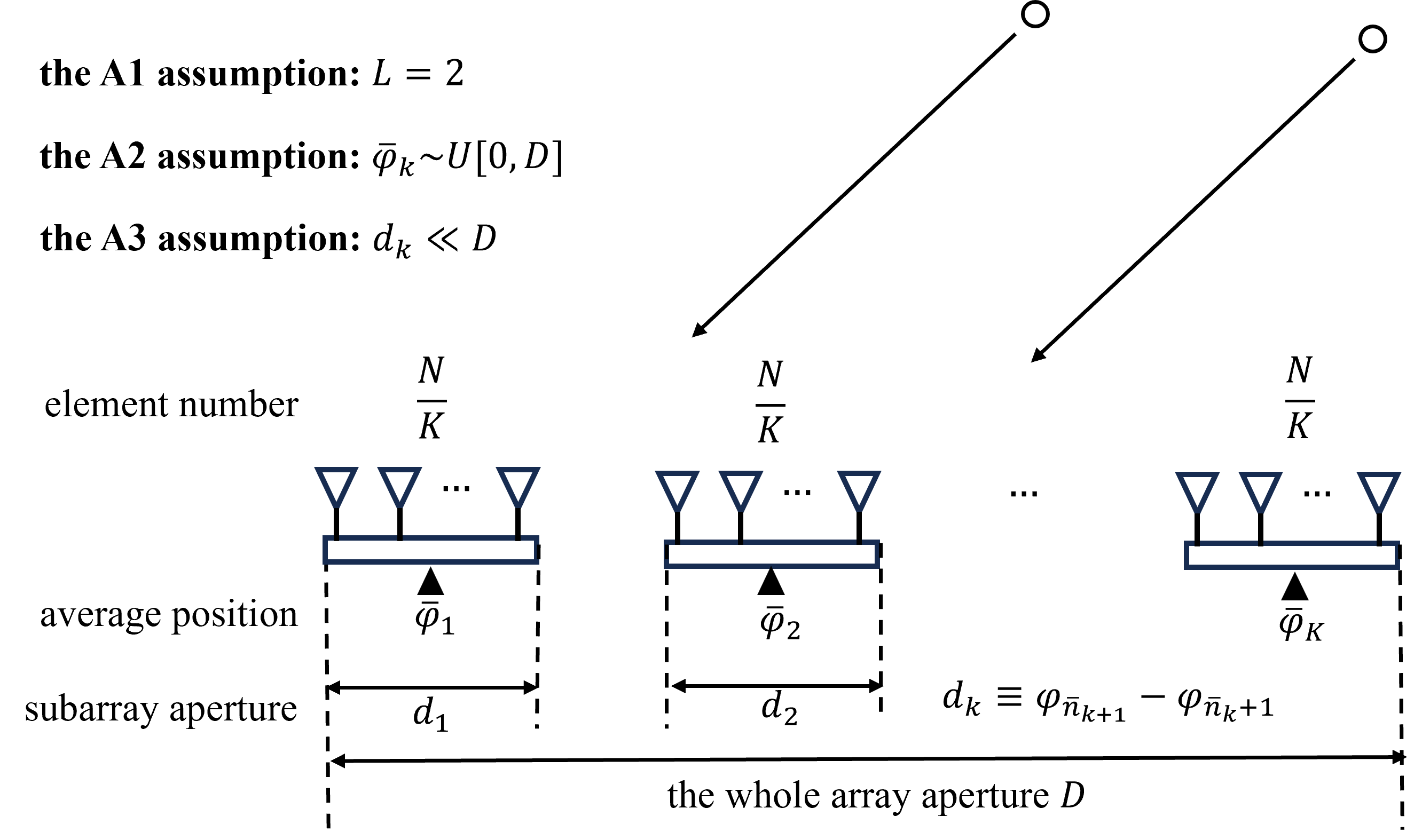
In Assumption A1, we mainly consider the case to simplify the expressions. In Assumption A2, uniformly distributed subarrays are common in practice. Note that Assumption 2 can be extended to more general cases, such as the case where the inter-subarray position errors are bounded instead of being distributed on the whole array aperture. These proofs are similar and we take Assumption A2 for example in this paper. In Assumption A3, we consider that the apertures of the subarrays, , are far less than the whole distributed array aperture , such that a subarray can be viewed as a point geometrically, i.e., for . In an extreme case, substituting for to (16) yields the corresponding equation. Therefore, closer intra-subarray displacements between implies smaller approximation errors in (16). This means that assumption A3 actually corresponds to a large, sparsely distributed array sensor network, which is usually used for high angular resolution.
V-B Proof of Proposition 2
The proof of Proposition 2 is not direct due to the complex form of w.r.t. . We then introduce intermediate variables w.r.t. , denoted by . We divide the proof of Proposition 2 into several tractable lemmas. In the sequel, we first introduce the intermediate variables and the lemmas, and then show how Proposition 2 is proved with these lemmas.
The intermediate variables are defined as
| (18) | ||||
| (19) |
where and . In the sequel, we abbreviate and as and , respectively. The intermediate variables correspond to the whole distributed array, and correspond to the -th subarray. Our theoretical results are mainly about , while are used for intermediate derivations. These intermediate variables are all bounded by 1. Abandoning extreme scenarios (), we assume
| (20) |
With the help of , we rewrite the CRB w.r.t. instead of , facilitating the analysis of the plateau phase. This is feasible because the proof of Lemma 2 and 3 is equivalent to that of Proposition 2:
and the lemmas are shown as follows. Lemma 2 shows that the intermediate variables and their derivatives w.r.t. tend to be zero when . The approximation to zero in Lemma 2 is a rough but intuitive expression, and the more rigorous expression is shown in the proof. Lemma 3 means that the main influence of on is embodied by , which supports the analysis of how affects instead.
Lemma 2.
Under assumptions A1-A3, when , we have
| (21) |
Proof.
See Appendix C. ∎
Here we give an intuitive explanation of how is close to 0 in Lemma 2. From Lemma 2. 1 in Appendix C, when , and , we have
| (22) |
The above conclusion can be extended to the cases of . Therefore, when is large enough, we have with high probability, yielding that Proposition 2 also holds with high probability.
Lemma 3.
Under assumptions A1-A3, when , we have
| (23) |
where .
Proof.
See Appendix D. ∎
Based on the chain rule of partial derivatives, we have
| (24) |
Substituting in Lemma 3 to (24) yields that
| (25) |
Under assumptions A1-A3, the Fisher information matrix (FIM) of CRB is not singular, yielding , where is some constant. Based on Lemma 2, we have when , which is also satisfied for since . Therefore, when we have
| (26) |
completing the proof.
V-C Proof of Proposition 3
The proof of Proposition 3 is similar to the counterpart of Proposition 2, except that Lemma 3 is replaced by Lemma 4, given by:
where Lemma 4 demonstrates that the main influence of on is embodied by :
Lemma 4.
Under assumptions A1-A3, when , we have
| (27) |
Proof.
See Appendix E. ∎
V-D Determining the turning point of CRB
We explain how to determine the turning of CRB. From the above propositions, we know that when , and decline rapidly as increases, and plateau out when . A criterion is in demand to distinguish the plateau phase and the declining phase in a strict sense, which implies the turning point of CRB.
As the CRB curve has the identical trend with the intermediate variables , by observing the structure of defined in (18), we use the criterion
| (28) |
to determine the turning point of CRB. Consequently, the turning point is located at
| (29) |
This criterion is inspired by [35], which considers a similar problem that distinguishes the correlated and uncorrelated signals, detailed as follows: Denote the correlation of two signals by ,
| (30) |
where is the frequency difference between two signals. The signals are regarded as correlated if is close to 1 or regarded as uncorrelated if approaches 0. In [35], it is explained that a sufficient condition for to be much less than one is that the integrand completes at least one cycle or equivalently
| (31) |
We use the similarity between in (18) and in (30) and determine the turning point of CRB as (29).
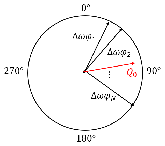
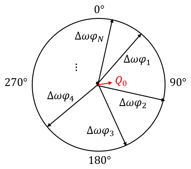
Finally, we give an intuitive explanation of this criterion applied in . Take as an example. When , we have , which means that the phases of are centralized in a small range of , yielding large . When , we have , which means that the phases of are distributed in and vectors in different directions cancel each other, yielding small . A diagram w.r.t. the phases of and is shown in Fig. 4 Since are the weighted extension of , they also approximately have the above characteristics.
VI Simulations
In this section, we first show the declining and plateau phases of and by the simulation results in Subsection VI-A, supporting the CRB analysis in Section IV. We present that the turning points of and are not sensitive to SNR in Subsection VI-B. We then give the approximation errors in the proof of Lemma 3 in Subsection VI-C to verify the feasibility of the approximation. Finally, we explain that high angular resolution is achievable for both fully and partly calibrated arrays by subspace based algorithms in Subsection VI-D, verifying our main conclusion.
VI-A Verification of the CRB analysis in Section IV
We show the declining and plateau phases of and w.r.t. by simulations to verify the theoretical analysis of CRB in Section IV.
Consider half-wavelength uniform linear subarrays, each composed of 10 elements, yielding . These subarrays are uniformly spaced on a straight line with for , where reflects the size of interval between subarrays and is set as . The wavelength of the received signals is , and the resolution limit of is thus . The geometry of the distributed array is shown in Fig. 5.
The directions are uniformly in the range of , i.e., for . In this case, we have , and denotes the minimum separation between sources. We set . The complex coefficients are set as for . The SNR is defined as being 20dB. We consider , and show and w.r.t. with a logarithmic coordinate in Fig. 6.
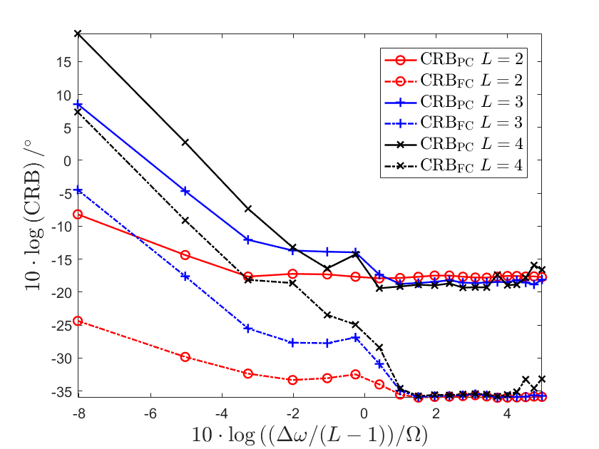
From Fig. 6, when , we find that the slopes of and w.r.t. in the cases are close to in the logarithmic coordinate, respectively. This verifies the conclusions in Lemma 1 and Proposition 1 that and are mainly proportional to when , which correspond to the declining phase of CRB. When , we find that and both begin to plateau out w.r.t. . This verifies the conclusions in Proposition 2 and Proposition 3, which correspond to the plateau phase of CRB.
Note that there is a fluctuation of CRB near the turning point, which is a common phenomenon in the CRB based resolution criterion. An intuitive reason is that the CRB involving the inverse of matrix usually has a complex form w.r.t. , particularly when is close to the resolution limit . Based on the theoretical analysis method proposed in this paper, we can also give a more convincing explanation on this phenomenon. Particularly, from the discussion in Subsection V-B and Subsection V-C, we transform the analysis of into that of . We take as an example and statistically analyze the how varies with . Based on the A1-A3 assumptions, we calculate the expectations of as follows.
| (32) |
This is a sinc function, where the most significant change of is reflected near , corresponding to the resolution cell . Since our study indicates that primarily influences the CRB in the form of , the significant variation of near indirectly results in the rapid fluctuation of around .
VI-B Verification of CRB turning point’s low sensitivity to SNR
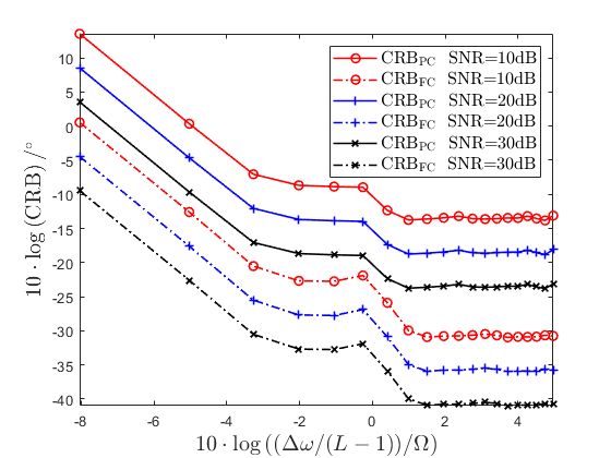
We show the turning points of and in different SNRs to explain that the proposed resolution criterion is not sensitive to noise.
Consider the same simulation setting as Subsection VI-A except . We plot the and curves for SNR being , , and dB, shown as Fig. 7. From Fig. 7, we find that the curves of in different SNRs have the same shapes, as well as the turning points. How the noise affects the CRB reflects on the absolute values of CRB, instead of the relative relationship between CRB and . This verifies that the proposed resolution criterion using the CRB turning point is not sensitive to SNR in Subsection IV-A.
VI-C Verification of the approximation in Lemma 3
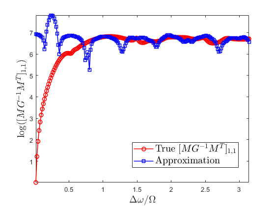
Since is the main component of different from , we show its approximation errors in the proof of Lemma 3. Particularly, we compare the approximate with the true counterpart.
Consider the same simulation setting as Subsection VI-A except . We take the (1,1) entries of the true and approximate as an example, and the comparison is shown in Fig. 8. From Fig. 8, we find that the approximation errors are large when , and become small when . This is because in the proof of Lemma 3, we use in Lemma 2 to simplify the proof. This conclusion is feasible for , but not for . When , the approximation results are close to the true values, yielding the feasibility of the approximation.
VI-D Similar angular resolution between fully and partly calibrated arrays
We show that the angular resolution of fully and partly calibrated arrays is similar, which is achieved by comparing the upper resolution limit of the corresponding direction-finding algorithms. Particularly, we provide the estimation accuracy of these algorithms varying with the source separation, and regard the turning point where the estimation accuracy initially tends to plateau out as the resolution limit. For fair comparison, the directions are estimated using Multiple Signal Classification (MUSIC) [38] for fully calibrated arrays, and root-RARE [4], spectral-RARE [5], and ESPRIT-GP [16] for partly calibrated arrays, since these algorithms are all based on subspace separation techniques with the difference being whether errors exist.
Consider the same simulation settings as Subsection VI-A except , the complex coefficients being standard Gaussian variables and the number of snapshots being . We use the root mean square error (RMSE) of to indicate the estimation performance of directions. We carry out Monte Carlo trials and denote the RMSE of by
| (33) |
where is the estimate in the -th trial and is the true value. The estimation results of MUSIC for fully calibrated arrays and root-RARE, spectral-RARE, and ESPRIT-GP for partly calibrated arrays w.r.t. are shown in Fig. 9.
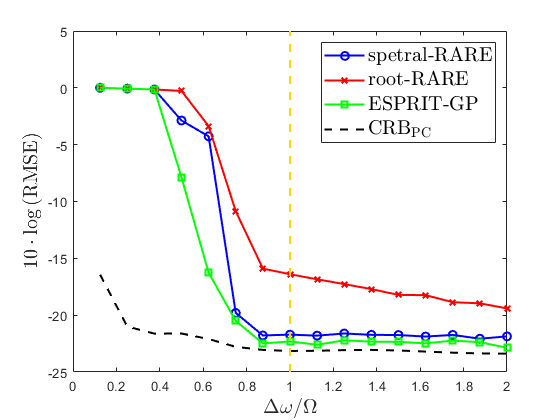
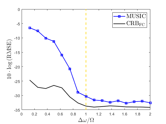
From Fig. 9(a), we find that when , the RMSEs of root-RARE, spectral-RARE, and ESPRIT-GP decline as increases; when , the RMSEs tend to be stable. Similar phenomenon is found in the fully calibrated case in Fig. 9(b), yielding that the resolution limit of these algorithms is close to . This also heuristically indicates that the resolution limit of fully and partly calibrated arrays is similar, both close to , corresponding to our main conclusion. We note that the turning points of the RMSEs w.r.t. in Fig. 9 are not exactly located at since is an empirical bound and the subspace based algorithms have super-resolution ability.
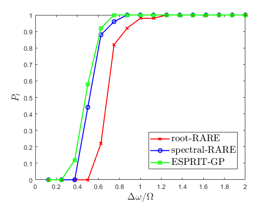
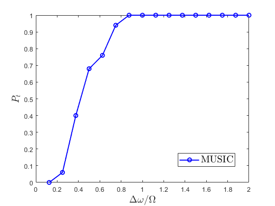
Then, we construct the dependence of the resolution probability for the RARE/ESPRIT methods in partly calibrated arrays and MUSIC method in fully calibrated arrays. Particularly, we define the resolution probability as the probability that the estimation error is less than a threshold, given by
| (34) |
where is the number of trials in which the estimation error is less than dB for partly calibrated case and dB for fully calibrated case, respectively, and the thresholds are empirically chosen based on the corresponding CRBs. The resolution probability of RARE/ESPRIT and MUSIC is shown as Fig. 10, which also verifies that the angular resolution between fully and partly calibrated arrays is similar.
VII Conclusion
In this paper, we theoretically explain that partly calibrated arrays achieve similar angular resolution as fully calibrated arrays, both inversely proportional to the whole array aperture. The analysis is based on a characteristics of CRB that when the source separation increases, the CRB w.r.t first declines rapidly, then plateaus out, and the turning point is close to the angular resolution limit. Hence, we transform the angular resolution analysis into comparing the turning points of the CRBs of fully and partly calibrated arrays, where the key technique lies in the partial derivative of CRB w.r.t. . To this end, we introduce some intermediate variables to simplify the analysis and theoretically explain the declining and plateau phases of the CRB. This work provides an important theoretical guarantee for the high-resolution performance of distributed arrays in mobile platforms. We believe that the proposed method to analyze the impact of position errors on resolution in distributed arrays using CRB turning points can be applied to other types of errors, such as gain and phase errors. This is theoretically feasible, but its specific implementation requires further research.
Appendix A Calculation of CRB
The CRBs of spatial frequencies using fully and partly calibrated arrays, denoted by and , respectively, are given by [4],
| (35) | ||||
| (36) |
where
| (37) |
| (38) |
| (39) |
| (40) |
| (41) |
| (42) |
| (43) |
| (44) |
We consider the single-snapshot case and omit since the multiple-snapshot cases () is a direct extension to those in the single-snapshot cases ().
Appendix B Proof of Proposition 1
The proof of Proposition 1 is an extension of Lemma 1 [25] from fully calibrated arrays to partly calibrated arrays. The main difference lies in the small quantity approximation of the matrix in (36).
Particularly, denote for and . When , we carry out Taylor expansion of in (44) on as
| (45) |
where and denotes the -order derivative of for . By substituting (B) to (44), we have
| (46) |
where .
From the proof of Lemma 1 [25], in (41) and in (40) w.r.t. are expressed as follows:
| (47) | ||||
| (48) |
where and are constants w.r.t. . Since in (40) is a symmetric projection matrix satisfying , we rewrite in (38) and in (39) respectively as
| (49) | ||||
| (50) |
By substituting (43), (48) and (46) to , we have
| (51) |
and is a constant w.r.t. , where and denotes the columns of for .
If (to be proved later), we substitute (47), (48) and (51) to (49) and (50), and have
| (52) | ||||
| (53) |
yielding that
| (54) |
where is a constant w.r.t. . Based on (54) and Lemma 1, we have (9) with
| (55) |
completing the proof.
Here we prove that any column of is not , hence : Consider if there is one column of equal to . We assume that the 1-st column of is without loss of generality, given by . In this case, we construct the following vector,
| (56) |
such that , where the the first , the second , and is expressed as [4]
| (57) |
with
| (58) | ||||
| (59) |
Since and in (57) is a projection matrix, should be in the column space of . However, we then explain that could not be in the column space of , i.e., there is no such that , yielding a contradiction. Particularly, define and denotes the rows of for . We find that has full column rank, given by
| (60) |
where . Therefore, there is no nonzero such that , yielding for any nonzero . This contradiction implies any column of is not and hence .
Appendix C Proof of Lemma 2
Lemma 2 in Subsection V-B is a rough representation, and we introduce its rigorous expression here, given by Lemma 2.1 and Lemma 2.2. For , we take as an example and the other cases are its direct extension with minor modifications.
For in Lemma 2, the rigorous expression is as follows:
Lemma 2. 1.
Under assumptions A1-A3, for any , define as
| (61) | ||||
| (62) |
When , we have
| (63) |
Proof.
For in Lemma 2, the rigorous expression is as follows:
Lemma 2. 2.
Under assumptions A1-A3, for any , when , we have
| (70) |
where are calculated for similar with for in Lemma 2. 1.
Proof.
The partial derivative of w.r.t. is
| (71) |
completing the proof. ∎
Appendix D Proof of Lemma 3
in (36) can be divided into and . The former is transformed into a function of in Lemma 4, and we consider the later one here.
To simply the derivation, we use the approximation in Lemma 2, and then substituting (94) to (38) and (39),
| (72) | ||||
| (73) |
where is a diagonal matrix denoted by .
Based on in Lemma 2 and in the A3 assumption (let ), by substituting (41) and (43) to (72), we approximate as
| (74) |
where , , and for .
Then, we approximate by , which is shown in the following lemma:
Lemma 5.
Based on Assumption A2, we have
| (75) |
where and .
Proof.
See Appendix F. ∎
Now, we approximate by
| (76) |
Define and . In the sequel, we discuss how and are recast as functions of , respectively. Based on the A1 assumption, and . We take the -th entry as an example, and the other entries can be directly derived. This is because the rows of have similar form, i.e.,
| (77) |
for .
For , substituting (D) and (5) to yields
| (78) |
where . Due to in (20), we have , yielding that
| (79) |
Consider the Taylor expansion of at , given by
| (80) |
By substituting (80) to (78), we have
| (81) |
where is denoted by
| (82) |
The effect of on in (81) is embodied in both and . In the sequel, we explain that is almost constant w.r.t. , which is detailed in the following lemma.
Lemma 6.
The gradient of w.r.t. , , satisfies
| (83) | ||||
| (84) |
Proof.
See Appendix G. ∎
Based on Lemma 6, when , we approximate by the constant , where . Since , we ignore the high-order terms of and approximate the infinite summation in (81) by its terms as
| (85) |
where for are given by , , , , , , respectively. Note that can be recast as
| (86) |
Substituting (86) to (D) yields
| (87) |
where and is a polynomial function w.r.t. and for , the specific form of which is omitted. Based on (16) in Assumption A3, we have
| (88) |
which can be directly recast as a polynomial function of for and , given by
| (89) |
where is a constant unrelated to , completing the proof of the part of .
For , substituting (5) to yields
| (90) |
Due to for any , (D) can be recast as
| (91) |
Similar as in (81), we substitute (43) and (D) to (D) and have
| (92) |
where for are expressed as and . Similar to the approximation on , we apply the procedures from (D) to (89) to in (D) and have
| (93) |
where is a constant unrelated to , completing the proof of the part of .
By combining the proofs on and , we complete the proof of this lemma.
Appendix E Proof pf Lemma 4
Appendix F Proof of Lemma 5
The following equation is satisfied, which can be directly verified by matrix multiplication:
| (101) |
where
| (102) |
| (103) |
where , and the matrix for .
When and , i.e., , we have
| (104) |
yielding when is large enough. The reason is shown as follows: Based on the A2 assumption, we have and is large (). By substituting (43) to , we have
| (105) |
where denotes a function of , and for , and the approximation in (F) is derived from . When , we have the conclusion in (104).
Based on Assumption A2, we have , which means
| (106) |
yielding in (103) with and , completing the proof.
Appendix G Proof of Lemma 6
The gradient of w.r.t. is calculated as
| (107) |
Since is either odd or even function of , we assume without loss of generality.
We prove the 1-st item in Lemma 6. Based on (107), (83) is equivalent to
| (108) |
Apply binomial expansion to the right part of (108), yielding
| (109) |
where
| (110) |
Since , for . Then, we prove that the left part of (108) is less than when , yielding the inequality of (108). Particularly, we have
| (111) |
for , completing the proof of the 1-st item in Lemma 6.
References
- [1] H. L. Van Trees, Optimum array processing: Part IV of detection, estimation, and modulation theory. John Wiley & Sons, 2004.
- [2] R. Heimiller, J. Belyea, and P. Tomlinson, “Distributed array radar,” IEEE Transactions on Aerospace and Electronic Systems, vol. AES-19, no. 6, pp. 831–839, 1983.
- [3] P. Stoica, M. Viberg, Kon Max Wong, and Qiang Wu, “Maximum-likelihood bearing estimation with partly calibrated arrays in spatially correlated noise fields,” IEEE Transactions on Signal Processing, vol. 44, no. 4, pp. 888–899, 1996.
- [4] M. Pesavento, A. B. Gershman, and K. M. Wong, “Direction finding in partly calibrated sensor arrays composed of multiple subarrays,” IEEE Transactions on Signal Processing, vol. 50, no. 9, pp. 2103–2115, 2002.
- [5] C. M. S. See and A. B. Gershman, “Direction-of-arrival estimation in partly calibrated subarray-based sensor arrays,” IEEE Transactions on Signal Processing, vol. 52, no. 2, pp. 329–338, 2004.
- [6] L. Lei, J. P. Lie, A. B. Gershman, and C. M. S. See, “Robust adaptive beamforming in partly calibrated sparse sensor arrays,” IEEE Transactions on Signal Processing, vol. 58, no. 3, pp. 1661–1667, 2010.
- [7] P. Parvazi, M. Pesavento, and A. B. Gershman, “Direction-of-arrival estimation and array calibration for partly-calibrated arrays,” in 2011 IEEE International Conference on Acoustics, Speech and Signal Processing (ICASSP), 2011, pp. 2552–2555.
- [8] C. Steffens, P. Parvazi, and M. Pesavento, “Direction finding and array calibration based on sparse reconstruction in partly calibrated arrays,” in 2014 IEEE 8th Sensor Array and Multichannel Signal Processing Workshop (SAM), 2014, pp. 21–24.
- [9] C. Steffens and M. Pesavento, “Block- and rank-sparse recovery for direction finding in partly calibrated arrays,” IEEE Transactions on Signal Processing, vol. 66, no. 2, pp. 384–399, 2018.
- [10] W. Suleiman, P. Parvazi, M. Pesavento, and A. M. Zoubir, “Non-coherent direction-of-arrival estimation using partly calibrated arrays,” IEEE Transactions on Signal Processing, vol. 66, no. 21, pp. 5776–5788, 2018.
- [11] G. Zhang, T. Huang, C. Chen, Y. Liu, X. Wang, and Y. C. Eldar, “Decentralized high-resolution direction finding in partly calibrated arrays,” Electronics letters, vol. 59, no. 4, p. e12741, 2023.
- [12] G. Zhang, T. Huang, C. Chen, Y. Li, Y. Liu, and X. Wang, “Fundamental limit of angular estimation using a distributed array with position and clock errors,” in 2023 IEEE 23rd International Conference on Communication Technology (ICCT). IEEE, 2023, pp. 69–73.
- [13] Y. Su, G. Zhang, T. Huang, Y. Liu, and X. Wang, “Direction finding in partly calibrated arrays using sparse bayesian learning,” in 2023 IEEE Radar Conference (RadarConf23). IEEE, 2023, pp. 01–06.
- [14] G. Zhang, T. Huang, Y. Liu, X. Wang, and Y. C. Eldar, “Direction finding in partly calibrated arrays exploiting the whole array aperture,” IEEE Transactions on Aerospace and Electronic Systems, vol. 59, no. 5, pp. 5978–5992, 2023.
- [15] P. Stoica and A. Nehorai, “Music, maximum likelihood, and cramer-rao bound,” IEEE Transactions on Acoustics, speech, and signal processing, vol. 37, no. 5, pp. 720–741, 1989.
- [16] B. Liao and S.-C. Chan, “Direction-of-arrival estimation in subarrays-based linear sparse arrays with gain/phase uncertainties,” IEEE Transactions on Aerospace and Electronic Systems, vol. 49, no. 4, pp. 2268–2280, 2013.
- [17] B. Liao and S. C. Chan, “Direction finding with partly calibrated uniform linear arrays,” IEEE Transactions on Antennas and Propagation, vol. 60, no. 2, pp. 922–929, 2011.
- [18] J. M. Merlo, S. R. Mghabghab, and J. A. Nanzer, “Wireless picosecond time synchronization for distributed antenna arrays,” IEEE Transactions on Microwave Theory and Techniques, vol. 71, no. 4, pp. 1720–1731, 2023.
- [19] H. Cox, “Resolving power and sensitivity to mismatch of optimum array processors,” The Journal of the acoustical society of America, vol. 54, no. 3, pp. 771–785, 1973.
- [20] K. Sharman and T. Durrani, “Resolving power of signal subspace methods for finite data lengths,” in ICASSP’85. IEEE International Conference on Acoustics, Speech, and Signal Processing, vol. 10. IEEE, 1985, pp. 1501–1504.
- [21] M. N. El Korso, R. Boyer, A. Renaux, and S. Marcos, “Statistical resolution limit for the multidimensional harmonic retrieval model: hypothesis test and cramér-rao bound approaches,” EURASIP Journal on Advances in Signal Processing, vol. 2011, no. 1, pp. 1–14, 2011.
- [22] C. Ren, M. N. E. Korso, J. Galy, E. Chaumette, P. Larzabal, and A. Renaux, “On the accuracy and resolvability of vector parameter estimates,” IEEE Transactions on Signal Processing, vol. 62, no. 14, pp. 3682–3694, 2014.
- [23] M. Sun, D. Jiang, H. Song, and Y. Liu, “Statistical resolution limit analysis of two closely spaced signal sources using rao test,” IEEE Access, vol. 5, pp. 22 013–22 022, 2017.
- [24] M. Thameri, K. Abed-Meraim, F. Foroozan, R. Boyer, and A. Asif, “On the statistical resolution limit (srl) for time-reversal based mimo radar,” Signal Processing, vol. 144, pp. 373–383, 2018.
- [25] H. B. Lee, “The cramér-rao bound on frequency estimates of signals closely spaced in frequency,” IEEE Transactions on Signal Processing, vol. 40, no. 6, pp. 1507–1517, 1992.
- [26] S. Smith, “Statistical resolution limits and the complexified cramér-rao bound,” IEEE Transactions on Signal Processing, vol. 53, no. 5, pp. 1597–1609, 2005.
- [27] H. Abeida and J.-P. Delmas, “Refinement and derivation of statistical resolution limits for circular or rectilinear correlated sources in ces data models,” Signal Processing, vol. 195, p. 108478, 2022.
- [28] Y. Wan, A. Liu, R. Du, and T. X. Han, “Fundamental limits and optimization of multiband sensing,” 2023. [Online]. Available: https://arxiv.org/abs/2207.10306
- [29] K. Usmani and B. Javidi, “Longitudinal resolution of three-dimensional integral imaging in the presence of noise,” Optics Express, vol. 32, no. 23, pp. 40 605–40 619, 2024.
- [30] S.-F. Yau and Y. Bresler, “Worst case cramer-rao bounds for parametric estimation of superimposed signals with applications,” IEEE Transactions on Signal Processing, vol. 40, no. 12, pp. 2973–2986, 1992.
- [31] M. P. Clark, “On the resolvability of normally distributed vector parameter estimates,” IEEE Transactions on Signal Processing, vol. 43, no. 12, pp. 2975–2981, 1995.
- [32] Z. Liu and A. Nehorai, “Statistical angular resolution limit for point sources,” IEEE Transactions on Signal Processing, vol. 55, no. 11, pp. 5521–5527, 2007.
- [33] R. Hansen, “Fundamental limitations in antennas,” Proceedings of the IEEE, vol. 69, no. 2, pp. 170–182, 1981.
- [34] Y. Wang and K. C. Ho, “Unified near-field and far-field localization for aoa and hybrid aoa-tdoa positionings,” IEEE Transactions on Wireless Communications, vol. 17, no. 2, pp. 1242–1254, 2018.
- [35] E. Fishler, A. Haimovich, R. S. Blum, L. J. Cimini, D. Chizhik, and R. A. Valenzuela, “Spatial diversity in radars—models and detection performance,” IEEE Transactions on signal processing, vol. 54, no. 3, pp. 823–838, 2006.
- [36] D. Malioutov, M. Cetin, and A. S. Willsky, “A sparse signal reconstruction perspective for source localization with sensor arrays,” IEEE transactions on signal processing, vol. 53, no. 8, pp. 3010–3022, 2005.
- [37] D. L. Donoho, “Compressed sensing,” IEEE Transactions on information theory, vol. 52, no. 4, pp. 1289–1306, 2006.
- [38] R. Schmidt, “Multiple emitter location and signal parameter estimation,” IEEE transactions on antennas and propagation, vol. 34, no. 3, pp. 276–280, 1986.
- [39] S. Boucheron, G. Lugosi, and O. Bousquet, “Concentration inequalities,” in Summer school on machine learning. Springer, 2003, pp. 208–240.