Functional regression clustering
Abstract
Gene expression data is often collected in time series experiments, under different experimental conditions. There may be genes that have very different gene expression profiles over time, but that adjust their gene expression patterns in the same way under experimental conditions. Our aim is to develop a method that finds clusters of genes in which the relationship between these temporal gene expression profiles are similar to one another, even if the individual temporal gene expression profiles differ. We propose a -means type algorithm in which each cluster is defined by a function-on-function regression model, which, inter alia, allows for multiple functional explanatory variables. We validate this novel approach through extensive simulations and then apply it to identify groups of genes whose diurnal expression pattern is perturbed by the season in a similar way. Our clusters are enriched for genes with similar biological functions, including one cluster enriched in both photosynthesis-related functions and polysomal ribosomes, which shows that our method provides useful and novel biological insights.
Keywords:
Autoregressive random errors; Circadian clock; Functional mixture clustering; Functional regression; Gene expression; -means.
1 Introduction
Next-generation sequencing technology (specifically RNA-sequencing or RNA-seq) allows researchers to accurately measure gene expression for all genes in a biological sample (Lister et al., 2008). Until recently, it was prohibitively expensive to perform RNA-seq experiments at more than a few time points at once. RNA-seq is now widespread and affordable enough to use it to investigate time-sensitive biological processes, such as response to environmental stimuli or the organism’s internal clock (Swift & Coruzzi, 2017). In this context, typical biological questions are to detect genes that are differentially expressed over time, and clustering genes according to their expression time courses. Such clustering efforts have mainly been focussed on finding subgroups of genes sharing common time course patterns (Ezer, Shepherd, Brestovitsky, Dickinson, Cortijo, Charoensawan, Box, Biswas, Jaeger & Wigge, 2017; Ezer, Jung, Lan, Biswas, Gregoire, Box, Charoensawan, Cortijo, Lai, Stöckle, Zubieta, Jaeger & Wigge, 2017).
In addition to single RNA-seq time-course experiments, it is now common to perform multiple time series RNA-seq experiments under multiple different treatments (Ezer, Shepherd, Brestovitsky, Dickinson, Cortijo, Charoensawan, Box, Biswas, Jaeger & Wigge, 2017; Ezer, Jung, Lan, Biswas, Gregoire, Box, Charoensawan, Cortijo, Lai, Stöckle, Zubieta, Jaeger & Wigge, 2017), and methods for analysing such data are not well-established. In this paper, we propose a fundamentally different approach to clustering such multiple gene expression time course, by using the link between them—through a functional regression—as a way of clustering genes. This strategy would be able to group together genes that may have very different temporal expression profiles in different conditions, but whose profiles change in the same way across treatments. We hypothesize that such genes would be part of the same pathways. For instance, two genes might have different gene expression patterns under normal growth conditions, because they are normally regulated by different sets of regulatory proteins. However, both these genes might be regulated by the same stress-associated regulatory protein in response to an environmental stimulus, which causes their gene expression pattern to be perturbed in the same way.
Our approach is based on treating gene expression time courses as curves that are sampled discretely, with measurement error, and falls therefore within the realm of functional data analysis (FDA: Ramsay & Silverman, 2005; Ferraty & Vieu, 2006; Horváth & Kokoszka, 2012; Hsing & Eubank, 2015; Kokoszka & Reimherr, 2017), now a prevalent area of statistics, with applications in numerous fields, such as in neuroimaging (Jiang et al., 2009; Zipunnikov et al., 2011; Ivanescu et al., 2015; Li et al., 2015; Jiang et al., 2016; Petersen et al., 2016; Rügamer et al., 2018; Palma et al., 2020), phonetics (Aston et al., 2010; Hadjipantelis et al., 2012, 2015; Pigoli et al., 2018; Tavakoli et al., 2019), or genomics (Serban & Wasserman, 2005; Yao et al., 2005; Reimherr et al., 2014; Ezer & Keir, 2019). Classical statistical modelling tools have been extended to functional data: the functional linear model (FLM) has received a lot of attention (see the review of Morris, 2015, and references therein), and many generalizations have been proposed, such as those inspired by generalized linear models (Müller & Stadtmüller, 2005), (generalized) additive models (Müller & Yao, 2008; McLean et al., 2014; Scheipl et al., 2016), or non-parametric regression (Ferraty & Vieu, 2006).
Parallel to this, there have been many contributions to the clustering of functional data: generalizations of -means have been proposed, usually after projecting the functional observations onto some finite basis of functions (Abraham et al., 2003; Serban & Wasserman, 2005; Auder & Fischer, 2012; Antoniadis et al., 2013), or onto the first functional principal components (FPC; Peng et al., 2008). Extensions of such functional -means have also been proposed: Chiou & Li (2007) proposed using the subspaces spanned by FPCs as representative of the clusters, instead of using cluster means to define the clusters, and Gattone & Rocci (2012) proposed a functional version of the reduced -means algorithm (De Soete & Carroll, 1994). Delaigle et al. (2019) proposed to choose adaptively the projections onto which the -means algorithm is applied, and showed that the technique can yield asymptotically perfect clustering. Mixture models for functional clustering have also been proposed (Chudova et al., 2004; Petrone et al., 2009; Schmutz et al., 2020).
Combining functional linear models and functional clustering has, however, been far less studied. Such a problem is motivated, for instance, by trying to find subgroups in the data characterized by different relationships between the (scalar or functional) response, and one or several functional covariates. An example of such problem arises in plant genomics, where one is interested in clustering the genes of a plant based on the relationship of its circadian expression in summer, say , where is a time observation in hours i.e. from a process observed during two entire days (and 0 represents midnight of the first day), and its relationship with the circadian expressions in autumn, winter and spring, say . In this setting, one could consider a cluster-specific functional linear model, such as
| (1) |
if gene belongs to group , where . The group memberships are of course unknown, but finding clusters based on model (1) is of interest, and gives promising results when applied to gene expressions timecourses of Arabidopsis halleri specimen, see Section 5.1.
To the best of our knowledge, only a handful of papers have considered clustering functional data using functional models similar to (1) Yao et al. (2011) looked at scalar-on-function regression modelling (i.e. the case in (1)) with one functional covariate, and used FPCA for regularization. Wang et al. (2016) considered the concurrent functional linear model if the observation comes from group , and used a mixture of Gaussian processes to fit the model using an EM-type algorithm. In this paper, we present a multivariate functional clustering method based on a cluster-specific functional linear model like (1), called Functional Regression Clustering (FRECL). It clusters data of the form , where are curves, and allowing . Our proposed method has been developed with the application to gene expression time courses in mind, but it can also be used in other applications, such as the multiple sclerosis applications of Ivanescu et al. (2015). Indeed, FRECL is versatile enough to be easily applied to cluster any data set in which multiple functional data sets are being compared.
The paper is organized as follows. In Section 2, we describe and present our FRECL model and method for finding the clusters and the regression surfaces . In Section 3, we provide a description of our motivating application for FRECL. In Section 4, we provide an extensive simulation study of the performance of our method in data that resembles that in our motivating example, and compare it to existing (functional) clustering methods. In Section 5, we identify clusters in an expression time course data set utilising FRECL. Section 6 concludes with a discussion. The full code of our method is made available for reproducing our results, and for further applications, see https://gitlab.com/sconde778/frmm_rpackagefunctions.git
2 Description of method
Given multivariate functional observations , where , where is the Hilbert space of square integrable functions defined over the compact interval , with norm , the goal of our paper is to cluster these observations into groups according to the relation between the responses , and the predictors . While we assume that the functional responses and predictors are all defined on the same domain , our methods can easily be extended to settings with distinct domains for the response and each predictors.
Let denote the set of partitions of into disjoint sets (which we shall call clusters), with elements of the form . Notice that we allow partitions with empty clusters, which implies that provided we identify sets of the form with , where are nonempty sets, . Let the indicator function of the set , defined by if , and otherwise. We assume that the observations come from the following model,
| (2) |
where is a fixed partition, is a functional error term, , and , , . In other words, the same functional linear model links and within each cluster , but the functional parameters are (possibly) distinct across the clusters . The goal is to find the unknown partition .
Letting be a functional vector, and defining
| (3) |
then (2) can be rewritten as
Another way of expressing model (2) is to say that the model
| (4) |
holds within each cluster of , with possibly distinct functional parameters . Note that it is not straightforward to view model (2) as a mixture model since density functions are generally not well defined in a functional context (Delaigle et al., 2010). Notice that (4) is a function on function regression model with multiple functional predictors, and that can be viewed as the conditional expectation of the functional response given and , provided .
Our strategy for finding is inspired by the -means algorithm (MacQueen et al., 1967), which we can view as an iterative procedure alternating between a model fitting (the computation of the cluster means given the cluster allocations) and a partition update (assigning each observation in the next iteration to the current closest cluster mean). We therefore propose to estimate using an iterative procedure, summarized as follows:
-
1.
Pick with non-empty clusters at random,
-
2.
Fit model (4) within each cluster of , thus obtaining fitted models,
-
3.
Reassign the th observation, to the best fitting model , thus defining a new partition ,
-
4.
Set and repeat steps 2–3 until convergence.
Notice that step 2 requires a fitting method . We discuss the choice of below. Step 2 results in fitted models of the form (4), with estimates . Step 3 requires finding the best fitting model for each observation ; we choose to do this by computing the norm of its fitted residuals under each model,
| (5) |
Other methods for updating clusters can be chosen, such as choosing a different norm in (5). The full version of our generic FRECL algorithm, using the fitting method , is given in Algorithm 1.
Because the output of Algorithm 1 depends on the initial random partition, we propose to use consensus clustering (Monti et al., 2003) to produce more consistent results. Consensus clustering consists of running a clustering algorithm multiple times, with different initial partitions, and then aggregating the obtained clusters. We describe it formally in Algorithm 2.
Algorithms 1 and 2 depend on a number of parameters, which we now briefly discuss and make recommendations about. A more detailed discussion of the choice of some of these parameters is deferred to Section 4.
Fitting method
Fitting functional linear models (FLM) involves solving ill-posed inverse problems, and requires some form of regularization, which is generally performed by projection of the functional observations on a finite number of functional principal components. This is usually performed either after transforming the discretely observed functional data into curves, or simultaneously, see Morris (2015); Greven & Scheipl (2017) for overviews of functional regression. A more recent approach to FLM is to use computational methods—such as boosting (Brockhaus et al., 2015)—for model fitting. Brockhaus et al. (2018) propose such approach, which is nicely implemented in the R package FDboost (Brockhaus & Ruegamer, 2018; R Core Team, 2020). In the rest of the paper, we use to be given by the R function FDboost. We will always work with the discretised curves and FDboost regularises automatically.
Stopping criterion
Currently, our stopping criteria is when (i) either convergence is reached, i.e. the partitions are the same between two consecutive iterations or alternatively (ii) the number of iterations has exceeded a fixed value which we set to 300. Several alternative approaches are possible. For instance, a stopping criteria may be very strict, such as “only stop iterations when either convergence or a cycle is reached.” It may also be possible to stop at some point which is approaching convergence, when only a small proportion of observations change clusters across an iteration. Our choice of stopping criteria is motivated by the analysis in Section 4.2.3.
Number of clusters
In order to determine the number of clusters, we propose to run the algorithm for a range of values of , and compute each time the mean squared error (MSE) with the residuals from the final partition:
| (6) |
where and is as in (5). We then plot those quantities and use an elbow-like criterion.
Number of runs for consensus clustering
The choice of depends on the balance between runtime and robustness. The larger the value of the longer it takes for the algorithm to complete, but the more consistent the clusters will be. We analyse the impact of varying this parameter in more depth in Section 4.2.4.
3 Motivating application
3.1 Biological background
FRECL can cluster any data set in which each observation consists of two or more functional data. However, we were specifically interested in developing this method to provide new biological insights related to how plant gene expression changes over time in response to the seasons. In our analysis, we aimed to find clusters of genes determined by associations between daily gene expression patterns during the summer, and those during autumn, winter and spring. Many agriculturally-relevant traits that are of interest to plant biologists, such as flowering, occur in the summer. However, many of the developmental decisions that lead to these traits are thought to occur in the other seasons. For instance, flowering time in the summer is determined by the temperature in winter (vernalisation) (Xu & Chong, 2018) and the changes in day length in the spring (photoperiod sensing) (Song et al., 2015; Brambilla et al., 2017).
About a third of genes are controlled by the circadian clock and vary their expression levels over the course of the day (Covington et al., 2008). Indeed, many of the key vernalisation and photoperiod sensing genes are known to be directly regulated by the circadian clock (Johansson & Staiger, 2015). In many species, the daily pattern of gene expression varies across different seasons because of differences in day length, vernalization and winter-dormancy (Song et al., 2012; Brambilla et al., 2017; Song et al., 2015). Even genes that are not regulated by the circadian clock may be more sensitive to environmental fluctuations, like pests, shade or UV light, during specific seasons (Ezer & Wigge, 2017). Also, some genes may play one biological role in one season and play another role in another season, especially genes involved in plant development and response to plant hormones.
Because of these properties, we thought that genes that are biologically associated with one another may have very different expression patterns, but may have similar gene expression changes across different seasons. If this were the case, we would expect FRECL to produce clusters of genes that share biological roles.
3.2 Description of data
The publicly available gene expression data Nagano et al. (2019) was collected to investigate how diurnal patterns of gene expression change in different seasons. It contains gene expressions of 32669 genes from an experiment done in Arabidopsis halleri specimens, a perennial relative of the model plant organism Arabidopsis thaliana. The expressions were measured via RNA-seq at four seasons (winter/summer solstice and spring/autumn equinox), over the course of 48 hours, sampled every other hour, with 5–6 replicates per time point. See additional details in Appendix 6.1.
3.3 Pre-processing data set
The following pre-processing steps were undertaken before this data was used in either Sections 4 or 5, below.
We computed the median gene expression value over the replicates per time point for each season. Then, we selected genes that were expressed above a threshold (specifically, those whose transcripts per million (TPM) was larger than ) in 20 or more time points in each season. This is a common threshold used in biology for filtering out very lowly expressed genes (Ezer & Wigge, 2017).
We transformed all the variables by subtracting, for each gene, the sample mean curve of all the gene expression, and then smoothed the resulting curve by using a loess smoother (Cleveland, 1979; Cleveland & Devlin, 1988), formed with local quadratic polynomials. For the th gene, let represents the (median, transformed, loess-ed) gene expression at time in summer, and let be its expressions in spring, autumn and winter for respectively. We drop the words “transformed, median, loess-ed” from now on. For computations, we used the evaluation each smoothed curve at the original set of time points.
In Section 4, we describe a simulation study that was designed so that the data had very similar properties to the motivating example. In Section 5, we apply FRECL to the real gene expression data set, and demonstrate that this method is useful for generating new biological insights and hypotheses for future investigations.
4 Simulations
4.1 Simulation strategy
4.1.1 Overview
We compare our method with these alternative approaches in a simulation study in Subsection 4.1.4. The simulated data was generated to represent realistic situations, so that the results would be applicable to real data. In order to generate a new simulated data set that shares many of the properties of the real one, we sample the explanatory variables and assign them to known partitions. Additionally, we use the explanatory and response variables to generate a set of realistic model parameters, which we sample from when we assign parameters to each partition. Finally, for each partition, the sampled explanatory variables and parameters are used to generate simulated response variables.
4.1.2 Generating the simulated data set.
We want to simulate data generated from the model in equation (2), using the real data described in sections 3.2 and 3.3. The model has then a functional response, which is the gene expression at summer, and explanatory variables, which are the gene expressions at spring, autumn and winter. We work with the discretized variables defined in the original set of time points . The time points, equidistant, are . First, we choose as the fitted parameters obtained by applying full FRECL (and using FDboost (Brockhaus et al., 2015; Brockhaus & Ruegamer, 2018) for fitting) to the real data , with equal to the number of desired clusters. Consequently, our choice of parameters represents a realistic situation. We then draw a partition at random, which will represent the true clusters. The FDboost package gives the discretised conditional expectation via the ‘predict’ routine – i.e. evaluated in . Finally, we construct the vector of the discretised simulated response , by adding errors varying across simulations.
Scenarios evaluated.
First, we consider the scenario composed by clusters, independent and identically distributed standard normal random error terms , and generate 50 simulations for sample sizes Additionally, we perform a sensitivity analysis for a variety of different scenarios. These include varying:
-
(i)
the distribution of the random error term from a discrete version of model (2). We consider two scenarios, both with and for . The first one with errors following an auto regressive model with 1 lag (AR1), i.e.
(7) where and the innovations are . The second one, with independent and identically distributed standard normal errors, i.e. .
-
(ii)
the number of clusters , with an analogous AR(1) random error term and for ;
-
(iii)
the sample size ;
-
(iv)
whether or norms are used in FRECL when computing the residuals in an iteration, see equation (5); we generate 50 simulations for each of the scenarios with these results are included in the supplementary material;
-
(v)
the number of iterations in the runs of one instance in Algorithm 1, for
-
(vi)
the number of runs, , , AR(1) random error term with .
(i)–(iii) are developed in Section 4.2.2, Figure 3 (i, iii) and Figure 4 (ii, iii); (iv) is developed in Section 4.2.3, Figure 5; (v) is developed in Section 4.2.4, Figure 6.
4.1.3 Metrics for evaluating accuracy
For each simulated data set, we compute the observed adjusted Rand Index (ARI; Hubert & Arabie, 1985), which allows for chance assuming that the underlying random variable defining the counts of pairs of observations belonging or not to clusters of the two partitions that are being compared is hypergeometric, the Rand index (Rand, 1971), which is the proportion of correctly classified pairs of observations selected at random, the true positive and the true negative clustering rates in the space of all pairs of observations. Specifically, we define a true positive and a true negative as the successful identification of a pair that are or are not part of the same cluster respectively.
4.1.4 Comparison with other methods
Whilst some FDA model developments involve multivariate functional data including at least a functional response and a functional explanatory variable (Chiou et al., 2016), FRECL is the only algorithm we are aware of that clusters observations based on the association between functional explanatory variables and functional response variables. However, there are a number of other methods for clustering functional data, which cluster the observations based on their (functional) response variables , i.e. ignoring .
We compare FRECL with five such methods. Because of our strategy for generating the simulated data, we would not expect to be involved in forming any discernible clusters (as these observations are randomly sampled), unlike (see Section 4 for more details). When comparing these methods on the real data, we consider observations formed with the values of both the explanatory and response, since might contain information pertinent for clustering and we did not wish to give FRECL an unfair advantage.
Firstly we compute the functional principal components (Ramsay & Silverman, 2005), done with a smooth of 12 B-spline basis of order 4 and equally spaced knots. The coefficients of the first principal components are clustered with the -means algorithm, and we select the that maximises the adjusted Rand Index (Hubert & Arabie, 1985). This optimal value of is, of course, unknown, but it can be used as an oracle. We call this method FPCA.oracle.
Secondly, High Dimensional Discriminant Clustering (HDDC), is based on Bergé et al. (2012) and described as filtering in Jacques & Preda (2014a) because the functional observations are approximated by a finite basis of functions. These assume a set of “multivariate” variables, formed in our context by the discrete set of time points. It is a model-based clustering focussed on a Gaussian Mixture model and using the expectation-maximisation algorithm for inference. We consider the default option, which implies selecting the dimension of the FPC space for each cluster using Cattell’s test. We call this clustering method HDDC.Cattell. We also consider an alternative to this method, by selecting the FPC space dimensions using the Bayesian Information Criterion (BIC) (Schwarz, 1978), and call this method HDDC.BIC.
Finally we consider FunHDDC (Schmutz et al., 2018; Bouveyron & Jacques, 2011) which is a generalisation of HDDC for functional data. It is adaptive because the coefficients of the bases of functions are assumed random variables having a cluster-specific probability distribution (Jacques & Preda, 2014a). It assumes an underlying latent functional mixture Gaussian model, where, unlike ours, the response is the only (functional) variable, and it models coefficients of basis expansions chosen to be the functional principal components from a cluster-specific analysis. These scores are assumed Gaussian with certain parameters. After estimating the dimensions of the FPC spaces, it is fitted with the EM algorithm. This method represents an extension of Jacques & Preda (2014b). When these dimensions are estimated with Cattell’s test, we call it as FunHDDC.Cattell. Otherwise, when considering the BIC, we call it as FunHDDC.BIC. We initialise the EM algorithm in the FunHDDC approaches with -means.
4.2 Simulation results
4.2.1 Simulations with 50 replicates and .
Figures 1 and 2 display boxplots with the distributions of the performance measures for the simulations with clusters, distance, i.i.d. random error model term, . In all the cases, FRECL outperforms any other method. It is the only method that as increases, the average performance measure does.
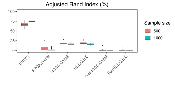


We also note that the FunHDDC approaches, which represent developments specific for clustering functional data, find the poorest results. This outcome is reversed in most of the scenarios of the AR(1) simulated models, see Table S1 in Supplementary File. A one-tailed -test indicates that the ARI in FRECL is a significant improvement over the alternative methods for any sample size ( for any ).
4.2.2 Results from sensitivity study.

Figure 3 compares simulations with a lag 1 autoregressive model to those from an independent and identically distributed error term; for FRECL and the five alternative methods. We note that the two simulated data sets here, for each of the sample sizes, were generated from functional models with the same . First, we see that FRECL, which is developed assuming a functional linear model, outperforms any other approach for any of the two simulations and sample sizes. FRECL, FPCA.oracle, FunHDDC.Cattell, and FunHDDC.BIC found greater mean ARI for the AR(1) models regardless of the sample size. Unlike HDDC.Cattell and HDDC.BIC, where the models with an i.i.d. error term have greater mean ARI for compared to For small sample size, FPCA.oracle and HDDC.BIC maximise the mean ARI in AR(1) and i.i.d. models (16.72% and 18.98% respectively). For big sample size, FunHDDC.BIC and HDDC.BIC outperform other alternative methods in AR(1) and i.i.d. models (19.98% and 16.71% respectively). FRECL performs outstandingly in all scenarios.

Figure 4 displays the observed ARI against simulations with clusters, on the horizontal axis, , for FRECL and the 5 alternative methods. Continuous and dotted lines indicate values for simulations with respectively. Overall, all the clustering performances decrease as the number of underlying clusters increases. FRECL outperforms any other approach in all instances. We tried the FunHDDC methods a number of times when these did not find a convergent model, in order to initialise differently the EM algorithm. If it was not possible to find a convergent model with clusters, we explored models with less number of clusters. Thus, FunHDDC.Cattell found a convergent model with 4 clusters for with either , with 2, 4 clusters for respectively, and ditto for FunHDDC.BIC found a model with 7 clusters for , with 5 clusters for and with 11 clusters for
4.2.3 Convergence properties of FRECL
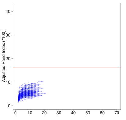
The first steps in FRECL consist of performing an iterative procedure a certain number of times prior to computing the consensus matrix. It is of interest to study the evolution of our performance measure of choice (e.g. the adjusted Rand index) for each iteration in a run. If we know that, in a particular scenario where FRECL computation has a lot of burden, as the number of iterations increases, it appears a plateau for our performance measure, then we can speed up the computations by shortening their number.
We computed the adjusted Rand index by iteration for a simulated data set in each of the scenarios: clusters, distance, , AR(1) random error terms. Figure 5 depicts the ARI in percentage form. Overall the ARI increases by iteration in all runs. We observed that it is monotonic increasing up to an iteration very close to the last one, e.g. the antepenultimate. When the number of clusters increases, the algorithm has less accurate performance. However, in this scenario the line approximately reaches a plateau when close to the iteration where convergence is achieved. In contrast, for small number of clusters, the values of the ARI increase very steeply towards the ‘end’ of the lines, suggesting that it is not advisable to shorten the number of iterations in these cases. As increases, the performance measures increases on average in either scenario.
 |
 |
| (a) | (b) |
 |
 |
| (c) | (d) |
4.2.4 The power of consensus clustering

When searching partitions with larger numbers of clusters, FRECL becomes computationally intensive. It is therefore of interest to investigate whether considering a small number of runs we can achieve an acceptable solution. For this purpose, we set up a study of the distributions of the adjusted Rand Index with different numbers of runs in one of our simulated data sets corresponding to a scenario with distance, AR(1). We computed the ARI for 20 groups of various numbers of runs, such that all the runs in these groups did not coincide with each other. And all this for 10, 20, 30, …, 100 runs as well as for 5 and 15 runs. Figure 6 includes boxplots of these distributions. The variability of the ARI decreases overall as the number of runs of the first stage in FRECL increases. Furthermore, on average it increases, and it becomes convergent from 20 or 30 runs on. This finding indicates that, first, consensus clustering is working because with bigger numbers of runs we obtain better performance, and moreover, we do not need to consider a big number of runs in order to accurately find a partition with a big number of clusters. A 0.05 level t-test gives poor evidence of any difference in the means (with a statistic of , 95% confidence interval of , p-value of ).
5 Application to new data to gain novel biological insight
5.1 Gene Seasonal Data Set
Our central aim was to identify sets of genes whose circadian gene expression profiles in the summer (during the flowering phase) was linked in the same way to gene expression in the autumn, winter, and spring. We expected that there would be modules of genes that may have very different expression patterns from one anotherF, but whose gene expression patterns change in the same way as the seasons progress.
FRECL was used to generate clusters in the seasonal A. halleri gene expression data sets previously described and the number of clusters was determined by the elbow method (see Figure 7(A)). We performed FRECL clustering twice: once using the gene expression profiles over two consecutive days, and once taking the average expression curve across the two days. In each setting, this produced 10 relatively evenly sized clusters (Figure 7(B)).


Genes in similar pathways do seem to group together in FRECL, suggesting that our method is a useful tool. In many model organisms, each gene is associated with a series of labels representing the cellular components, molecular functions, and biological processes that the protein encoded by the gene is involved in; these are referred to as gene ontology (GO) terms. For every A. halleri gene clustered by FRECL, we identified the most similar gene in the model plant Arabidopsis thaliana and searched for GO terms that were significantly associated with each cluster using gProfiler (Raudvere et al., 2019). We successfully identified a number of GO terms that were specific to certain gene clusters, see supplementary spreadsheet for a summary, which indicates that FRECL produces biologically interesting clusters. The adjusted p-values of a few key GO terms are illustrated in Figure 8. Interestingly, we find that ribosome and photosynthesis related genes tend to cluster together in FRECL, which may suggest that the same set of genes regulates the season-dependent gene expression of both processes, suggesting an avenue of research for biologists. We also observe cluster-specific enrichment in polysome, mRNA processing, and immunity-related processes.
The clusters produced by FRECL are very different from those produced by other methods, based on the ARI between the clusters produced by different clustering methods (Tables S5), indicating that our method potentially provides new biological insight. In fact, similarity in clustering algorithms was quite low (Tables S5 and S7 in the supplementary file), suggesting that each of these methods produces very distinct clusters in the real data, perhaps indicating that the partition to clusters in this data is highly dependent on how clusters are defined. A unique aspect of FRECL in comparison to other clustering algorithms is that FRECL clusters on the basis on the relationship between curves, and not only their shape. Indeed, we observe that genes that are assigned to the same cluster do not have similar gene expression patterns with each other, despite sharing GO terms (Figure 8).
Additionally, we were interested in determining whether FRECL provides biological information that can can help us identify gene pairs that share biological roles that would not have been identified using existing clustering methods. There were 184,605 pairs of genes that were found to be in the same clusters in FRECL, but not in any of the other methods (or 301,596 pairs when the average curve was used for clustering). Of these pairs, 169,605 were between pairs of genes whose orthologs in A. thaliana were included in AraNet, a gene network in Arabidopsis that uses a Bayesian approach to combine -omics data sets from various organisms to predict functional associations between pairs of genes in Arabidopsis (Lee et al., 2015; Lee & Lee, 2017) (or 278207 pairs when the average curve was used for clustering). 1470 of the novel pairwise associations found using FRECL but not in any of the other alternative clustering methods were found to be associated with one another in AraNet (or 2330 pairs when the average curve was used).
6 Discussion
Whilst Schmutz et al. (2018) claim that FunHDDC, a ‘specific’ method for clustering multivariate functional data, also works for univariate functional data, our simulation results show that it is outperformed by the other approaches we consider; even by those developed for non-functional, high dimensional variables such as HDDC. In one of the illustrations included in Bouveyron & Jacques (2011), FunHDDC is outperformed by HDDC, too.
Functional mixture models make possible to study relationships between explanatory and response variables over time allowing for clusters characterized by these relationships. Chamroukhi (2015) presents a clustering method for mixture regression that involves a penalised likelihood, where the penalty is the total entropy. FRECL is an alternative to these settings that does not need to consider a constrained optimization problem, and consequently does not need to estimate the value of the Lagrange multiplier. Yao et al. (2011) propose a functional mixture model implemented with FPCs in order to overcome overfitting with a finite number of observations and infinite-dimensional parameters and as usual selecting a certain number of components. The FPCs are necessarily computed (only) with the explanatory variables. Since the estimation of the slope parameters involves only the same number of selected FPCs, as well, the slope parameter space is restricted, and thus their estimates may be far from the truth. FRECL, clustering based on the functional ‘mixture’ model (2), improves existing methods, although these were not developed specifically for generating processes with an underlying functional mixture model. Consequently, it is a step further in the development of functional data clustering.
Software
Software in the form of R code, together with a sample input data set and complete documentation is available at https://gitlab.com/sconde778/frmm_rpackagefunctions.git.
Acknowledgments
Conflict of Interest: None declared. The authors thank Ioannis Kosmidis for suggesting appropriate venues for this manuscript. This project was funded by the Alan Turing Institute Research Fellowship under EPSRC Research grant (TU/A/000017) to DE; EPSRC/BBSRC Innovation Fellowship (EP/S001360/1) to DE and SC. ST would like to thank the Isaac Newton Institute for Mathematical Sciences, Cambridge, for support and hospitality during the programme Statistical Scalability where work on this paper was undertaken. This work was supported by EPSRC grant no EP/R014604/1.
References
- (1)
- Abraham et al. (2003) Abraham, C., Cornillon, P.-A., Matzner-Løber, E. & Molinari, N. (2003), ‘Unsupervised curve clustering using b-splines’, Scandinavian journal of statistics 30(3), 581–595.
- Antoniadis et al. (2013) Antoniadis, A., Brossat, X., Cugliari, J. & Poggi, J.-M. (2013), ‘Clustering functional data using wavelets’, International Journal of Wavelets, Multiresolution and Information Processing 11(01), 1350003.
- Aston et al. (2010) Aston, J., Chiou, J.-M. & Evans, J. (2010), ‘Linguistic pitch analysis using functional principal component mixed effect models’, Journal of the Royal Statistical Society: Series C (Applied Statistics) 59(2), 297–317.
- Auder & Fischer (2012) Auder, B. & Fischer, A. (2012), ‘Projection-based curve clustering’, Journal of Statistical Computation and Simulation 82(8), 1145–1168.
-
Bergé et al. (2012)
Bergé, L., Bouveyron, C. & Girard, S. (2012), ‘HDclassif: An R Package for Model-Based Clustering
and Discriminant Analysis of High-Dimensional Data’, Journal of
Statistical Software 46(6), 1–29.
http://jstatsoft.org/ -
Bouveyron & Jacques (2011)
Bouveyron, C. & Jacques, J. (2011), ‘Model-based clustering of time series in group-specific functional
subspaces’, Advances in Data Analysis and Classification 5(4), 281–300.
https://link.springer.com/article/10.1007/s11634-011-0095-6 - Brambilla et al. (2017) Brambilla, V., Gomez-Ariza, J., Cerise, M. & Fornara, F. (2017), ‘The importance of being on time: Regulatory networks controlling photoperiodic flowering in cereals’.
-
Brockhaus & Ruegamer (2018)
Brockhaus, S. & Ruegamer, D. (2018), FDboost: Boosting Functional Regression Models.
R package version 0.3-2.
https://github.com/boost-R/FDboost -
Brockhaus et al. (2018)
Brockhaus, S., Rügamer, D. & Greven, S. (2018), ‘Boosting Functional Regression Models with
FDboost’, arXiv:1705.10662 pp. 1–50.
https://arxiv.org/abs/1705.10662 -
Brockhaus et al. (2015)
Brockhaus, S., Scheipl, F., Hothorn, T. & Greven, S.
(2015), ‘The functional linear array
model’, Statistical Modelling 15(3), 279–300.
https://journals.sagepub.com/doi/abs/10.1177/1471082X14566913 -
Chamroukhi (2015)
Chamroukhi, F. (2015), ‘Unsupervised
learning of regression mixture models with unknown number of components’,
Journal of Statistical Computation and Simulation 86(12), 2308–2334.
https://www.tandfonline.com/doi/full/10.1080/00949655.2015.1109096 - Chiou & Li (2007) Chiou, J.-M. & Li, P.-L. (2007), ‘Functional clustering and identifying substructures of longitudinal data’, Journal of the Royal Statistical Society: Series B (Statistical Methodology) 69(4), 679–699.
- Chiou et al. (2016) Chiou, J.-M., Yang, Y.-F. & Chen, Y.-T. (2016), ‘Multivariate functional linear regression and prediction’, Journal of Multivariate Analysis 146, 301–312.
- Chudova et al. (2004) Chudova, D., Hart, C., Mjolsness, E. & Smyth, P. (2004), Gene expression clustering with functional mixture models, in ‘Advances in Neural Information Processing Systems’, pp. 683–690.
-
Cleveland (1979)
Cleveland, W. S. (1979), ‘Robust Locally
Weighted Regression and Smoothing Scatterplots’, Journal of the
American Statistical Association 74(368), 829–836.
http://www.jstor.org/stable/2286407[url cleveland79].
http://www.jstor.org/stable/2286407 -
Cleveland & Devlin (1988)
Cleveland, W. S. & Devlin, S. J. (1988), ‘Locally Weighted Regression: An Approach to
Regression Analysis by Local Fitting’, Journal of the American
Statistical Association 83(403), 596–610.
http://www.jstor.org/stable/2289282[url clevelanddevlin88].
http://www.jstor.org/stable/2289282 - Covington et al. (2008) Covington, M. F., Maloof, J. N., Straume, M., Kay, S. A. & Harmer, S. L. (2008), ‘Global transcriptome analysis reveals circadian regulation of key pathways in plant growth and development’, Genome Biology 9(1), R130.
- De Soete & Carroll (1994) De Soete, G. & Carroll, J. D. (1994), K-means clustering in a low-dimensional euclidean space, in ‘New approaches in classification and data analysis’, Springer, pp. 212–219.
- Delaigle et al. (2019) Delaigle, A., Hall, P. & Pham, T. (2019), ‘Clustering functional data into groups by using projections’, Journal of the Royal Statistical Society: Series B (Statistical Methodology) 81(2), 271–304.
- Delaigle et al. (2010) Delaigle, A., Hall, P. et al. (2010), ‘Defining probability density for a distribution of random functions’, The Annals of Statistics 38(2), 1171–1193.
- Ezer, Jung, Lan, Biswas, Gregoire, Box, Charoensawan, Cortijo, Lai, Stöckle, Zubieta, Jaeger & Wigge (2017) Ezer, D., Jung, J. H., Lan, H., Biswas, S., Gregoire, L., Box, M. S., Charoensawan, V., Cortijo, S., Lai, X., Stöckle, D., Zubieta, C., Jaeger, K. E. & Wigge, P. A. (2017), ‘The evening complex coordinates environmental and endogenous signals in Arabidopsis’, Nature Plants 3(7), 17087.
- Ezer & Keir (2019) Ezer, D. & Keir, J. (2019), ‘Nitpicker: selecting time points for follow-up experiments’, BMC bioinformatics 20(1), 166.
- Ezer, Shepherd, Brestovitsky, Dickinson, Cortijo, Charoensawan, Box, Biswas, Jaeger & Wigge (2017) Ezer, D., Shepherd, S. J., Brestovitsky, A., Dickinson, P., Cortijo, S., Charoensawan, V., Box, M. S., Biswas, S., Jaeger, K. & Wigge, P. A. (2017), ‘The G-box transcriptional regulatory code in Arabidopsis’, Plant Physiology 175(2), 628–640.
- Ezer & Wigge (2017) Ezer, D. & Wigge, P. A. (2017), ‘Plant Physiology: Out in the Midday Sun, Plants Keep Their Cool’, 27(1), PR28–R30.
- Ferraty & Vieu (2006) Ferraty, F. & Vieu, P. (2006), Nonparametric Functional Data Analysis: Theory and Practice, Springer.
- Gattone & Rocci (2012) Gattone, S. A. & Rocci, R. (2012), ‘Clustering curves on a reduced subspace’, Journal of Computational and Graphical Statistics 21(2), 361–379.
- Greven & Scheipl (2017) Greven, S. & Scheipl, F. (2017), ‘A general framework for functional regression modelling’, Statistical Modelling 17(1-2), 1–35.
- Hadjipantelis et al. (2012) Hadjipantelis, P., Aston, J. & Evans, J. P. (2012), ‘Characterizing fundamental frequency in mandarin: A functional principal component approach utilizing mixed effect models’, The Journal of the Acoustical Society of America 131(6), 4651–4664.
- Hadjipantelis et al. (2015) Hadjipantelis, P., Aston, J., Müller, H.-G. & Evans, J. P. (2015), ‘Unifying amplitude and phase analysis: A compositional data approach to functional multivariate mixed-effects modeling of mandarin chinese’, Journal of the American Statistical Association 110(510), 545–559.
- Horváth & Kokoszka (2012) Horváth, L. & Kokoszka, P. (2012), Inference for Functional Data with Applications, Springer.
- Hsing & Eubank (2015) Hsing, T. & Eubank, R. (2015), Theoretical Foundations of Functional Data Analysis, with an Introduction to Linear Operators, Wiley.
- Hubert & Arabie (1985) Hubert, L. & Arabie, P. (1985), ‘Comparing Partitions’, Journal of Classification 2, 193–218.
- Ivanescu et al. (2015) Ivanescu, A. E., Staicu, A.-M., Scheipl, F. & Greven, S. (2015), ‘Penalized function-on-function regression’, Computational Statistics 30(2), 539–568.
- Jacques & Preda (2014a) Jacques, J. & Preda, C. (2014a), ‘Functional data clustering: a survey’, Adv Data Anal Classif 8, 231–255.
- Jacques & Preda (2014b) Jacques, J. & Preda, C. (2014b), ‘Model based clustering for multivariate functional data’, Computational Statistics and Data Analysis 71, 92–106.
- Jiang et al. (2009) Jiang, C.-R., Aston, J. & Wang, J.-L. (2009), ‘Smoothing dynamic positron emission tomography time courses using functional principal components’, NeuroImage 47(1), 184–193.
- Jiang et al. (2016) Jiang, C.-R., Aston, J. & Wang, J.-L. (2016), ‘A functional approach to deconvolve dynamic neuroimaging data’, Journal of the American Statistical Association 111(513), 1–13.
- Johansson & Staiger (2015) Johansson, M. & Staiger, D. (2015), ‘Time to flower: Interplay between photoperiod and the circadian clock’, Journal of Experimental Botany 66(3), 719–730.
- Kokoszka & Reimherr (2017) Kokoszka, P. & Reimherr, M. (2017), Introduction to functional data analysis, CRC Press.
- Lee & Lee (2017) Lee, T. & Lee, I. (2017), AraNet: A network biology server for Arabidopsis thaliana and other non-model plant species, in ‘Methods in Molecular Biology’.
- Lee et al. (2015) Lee, T., Yang, S., Kim, E., Ko, Y., Hwang, S., Shin, J., Shim, J. E., Shim, H., Kim, H., Kim, C. & Lee, I. (2015), ‘AraNet v2: An improved database of co-functional gene networks for the study of Arabidopsis thaliana and 27 other nonmodel plant species’, Nucleic Acids Research 43(Database Issue), D996–1002.
- Li et al. (2015) Li, M., Staicu, A.-M. & Bondell, H. D. (2015), ‘Incorporating covariates in skewed functional data models’, Biostatistics 16(3), 413–426.
- Lister et al. (2008) Lister, R., O’Malley, R. C., Tonti-Filippini, J., Gregory, B. D., Berry, C. C., Millar, A. H. & Ecker, J. R. (2008), ‘Highly Integrated Single-Base Resolution Maps of the Epigenome in Arabidopsis’, Cell 133(3), 523–536.
- MacQueen et al. (1967) MacQueen, J. et al. (1967), Some methods for classification and analysis of multivariate observations, in ‘Proceedings of the fifth Berkeley symposium on mathematical statistics and probability’, Vol. 1, Oakland, CA, USA, pp. 281–297.
- McLean et al. (2014) McLean, M. W., Hooker, G., Staicu, A.-M., Scheipl, F. & Ruppert, D. (2014), ‘Functional generalized additive models’, Journal of Computational and Graphical Statistics 23(1), 249–269.
- Monti et al. (2003) Monti, S., Tamayo, P., Mesirov, J. & Golub, T. (2003), ‘Consensus clustering: a resampling-based method for class discovery and visualization of gene expression microarray data’, Machine Learning 52(1), 91–118.
- Morris (2015) Morris, J. (2015), ‘Functional regression’, Annual Review of Statistics and Its Application 2, 321–359.
- Müller & Stadtmüller (2005) Müller, H.-G. & Stadtmüller, U. (2005), ‘Generalized functional linear models’, the Annals of Statistics 33(2), 774–805.
- Müller & Yao (2008) Müller, H.-G. & Yao, F. (2008), ‘Functional additive models’, Journal of the American Statistical Association 103(484), 1534–1544.
- Nagano et al. (2019) Nagano, A. J., Kawagoe, T., Sugisaka, J., Honjo, M. N., Iwayama, K. & Kudoh, H. (2019), ‘Annual transcriptome dynamics in natural environments reveals plant seasonal adaptation’, Nature Plants 5, 74–83.
-
Palma et al. (2020)
Palma, M., Tavakoli, S., Brettschneider, J. & Nichols, T.
(2020), ‘Quantifying uncertainty in
brain-predicted age using scalar-on-image quantile regression’, NeuroImage 219, 116938.
http://www.sciencedirect.com/science/article/pii/S1053811920304249 - Peng et al. (2008) Peng, J., Müller, H.-G. et al. (2008), ‘Distance-based clustering of sparsely observed stochastic processes, with applications to online auctions’, The Annals of Applied Statistics 2(3), 1056–1077.
- Petersen et al. (2016) Petersen, A., Zhao, J., Carmichael, O. & Müller, H.-G. (2016), ‘Quantifying individual brain connectivity with functional principal component analysis for networks’, Brain connectivity 6(7), 540–547.
- Petrone et al. (2009) Petrone, S., Guindani, M. & Gelfand, A. (2009), ‘Hybrid dirichlet mixture models for functional data’, Journal of the Royal Statistical Society: Series B (Statistical Methodology) 71(4), 755–782.
- Pigoli et al. (2018) Pigoli, D., Hadjipantelis, P., Coleman, J. & Aston, J. (2018), ‘The statistical analysis of acoustic phonetic data: exploring differences between spoken romance languages’, Journal of the Royal Statistical Society (Series C) 67(5), 1103–1145.
-
R Core Team (2020)
R Core Team (2020), R: A Language and
Environment for Statistical Computing, R Foundation for Statistical
Computing, Vienna, Austria.
https://www.R-project.org/ -
Ramsay et al. (2020)
Ramsay, J. O., Graves, S. & Hooker, G. (2020), fda: Functional Data Analysis.
R package version 5.1.5.1.
https://CRAN.R-project.org/package=fda - Ramsay & Silverman (2005) Ramsay, J. & Silverman, B. W. (2005), Functional Data Analysis, Springer.
- Rand (1971) Rand, W. M. (1971), ‘Objective Criteria for the Evaluation of Clustering Methods’, Journal of the Americal Statistical Association 66(336), 846–850.
- Raudvere et al. (2019) Raudvere, U., Kolberg, L., Kuzmin, I., Arak, T., Adler, P., Peterson, H. & Vilo, J. (2019), ‘G:Profiler: A web server for functional enrichment analysis and conversions of gene lists (2019 update)’, Nucleic Acids Research 47(W1), W191–W198.
- Reimherr et al. (2014) Reimherr, M., Nicolae, D. et al. (2014), ‘A functional data analysis approach for genetic association studies’, The Annals of Applied Statistics 8(1), 406–429.
- Rügamer et al. (2018) Rügamer, D., Brockhaus, S., Gentsch, K., Scherer, K. & Greven, S. (2018), ‘Boosting factor-specific functional historical models for the detection of synchronisation in bioelectrical signals’, Journal of the Royal Statistical Society (Series C) 67(3), 621–642.
- Scheipl et al. (2016) Scheipl, F., Gertheiss, J. & Greven, S. (2016), ‘Generalized functional additive mixed models’, Electronic Journal of Statistics 10(1), 1455–1492.
-
Schmutz & Bouveyron (2019)
Schmutz, A. & Bouveyron, J. J. . C. (2019), funHDDC: Univariate and Multivariate Model-Based
Clustering in Group-Specific Functional Subspaces.
R package version 2.3.0.
https://CRAN.R-project.org/package=funHDDC -
Schmutz et al. (2018)
Schmutz, A., Jacques, J., Bouveyron, C., Chèze, L. & Martin, P.
(2018), Clustering multivariate functional
data in group-specific functional subspaces.
working paper or preprint.
https://hal.inria.fr/hal-01652467 - Schmutz et al. (2020) Schmutz, A., Jacques, J., Bouveyron, C., Cheze, L. & Martin, P. (2020), ‘Clustering multivariate functional data in group-specific functional subspaces’, Computational Statistics pp. 1–31.
-
Schwarz (1978)
Schwarz, G. (1978), ‘Estimating the
Dimension of a Model’, Annals of Statistics 6(2), 461–464.
https://www.andrew.cmu.edu/user/kk3n/simplicity/schwarzbic.pdf - Serban & Wasserman (2005) Serban, N. & Wasserman, L. (2005), ‘Cats: clustering after transformation and smoothing’, Journal of the American Statistical Association 100(471), 990–999.
- Song et al. (2012) Song, J., Angel, A., Howard, M. & Dean, C. (2012), ‘Vernalization - a cold-induced epigenetic switch’, Journal of Cell Science 125(1), 3723–3731.
- Song et al. (2015) Song, Y. H., Shim, J. S., Kinmonth-Schultz, H. A. & Imaizumi, T. (2015), ‘Photoperiodic flowering: Time measurement mechanisms in leaves’, Annual Review of Plant Biology 66(1), 441–464.
- Swift & Coruzzi (2017) Swift, J. & Coruzzi, G. M. (2017), ‘A matter of time — How transient transcription factor interactions create dynamic gene regulatory networks’, 1860(1), 75–83.
- Tavakoli et al. (2019) Tavakoli, S., Pigoli, D., Aston, J. A. & Coleman, J. (2019), ‘A spatial modeling approach for linguistic object data: Analysing dialect sound variations across Great Britain’, Journal of the American Statistical Association 114(527), 1081–1096.
- Wang et al. (2016) Wang, S., Huang, M., Wu, X. & Yao, W. (2016), ‘Mixture of functional linear models and its application to co2-gdp functional data’, Computational Statistics & Data Analysis 97, 1–15.
-
Xu & Chong (2018)
Xu, S. & Chong, K. (2018),
‘Remembering winter through vernalisation’, Nature Plants 4, 997–1009.
https://www.nature.com/articles/s41477-018-0301-z -
Yao et al. (2011)
Yao, F., Fu, Y. & Lee, T. C. M. (2011), ‘Functional mixture regression’, Biostatistics .
http://biostatistics.oxfordjournals.org - Yao et al. (2005) Yao, F., Müller, H.-G. & Wang, J.-L. (2005), ‘Functional Data Analysis for Sparse Longitudinal Data’, Journal of the American Statistical Association 100(470), 577–590.
- Zipunnikov et al. (2011) Zipunnikov, V., Caffo, B., Yousem, D., Davatzikos, C., Schwartz, B. S. & Crainiceanu, C. (2011), ‘Functional principal component model for high-dimensional brain imaging’, NeuroImage 58(3), 772–784.
Appendix
6.1 Data
The seasonal data set contains 3 replicates per time points in autumn and 4 replicates for all the other time points for 32745 genetic entities, 32669 of which are genes. The expression for the th gene is the observed proportion of messenger RNAs of the th gene from specimen X over the total of mRNAs in specimen X multiplied by . We removed one suspicious replicate in a time point; it has zero values in many of the genes. If included, the line plots of many of the raw spring gene expressions have a very odd minimum at a time point. We computed the median gene expression per time point as, if using the mean, there are a lot of “ups and downs” in nearby time points. We selected genes whose median expression was units except at most 5 time points in each of the 4 seasons. The first time points are collected at 16:00 hours in spring (March, days 19-21), summer (June, days 26-28), autumn (September, 24-26) and winter (December, 24-26). With these criteria, the resulting data set has genes.