Fully Understanding Generic Objects:
Modeling, Segmentation, and Reconstruction
Abstract
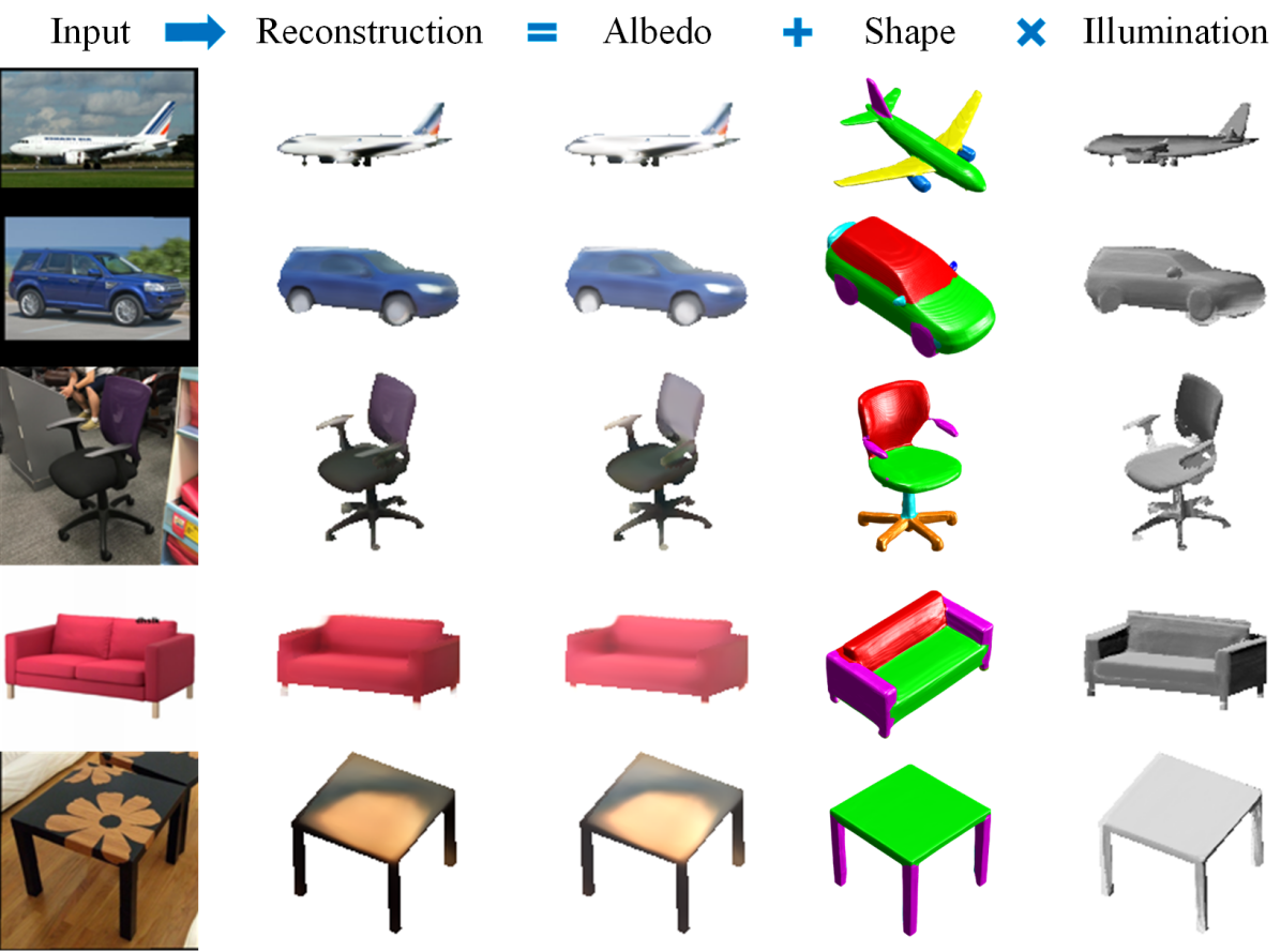
Inferring D structure of a generic object from a D image is a long-standing objective of computer vision. Conventional approaches either learn completely from CAD-generated synthetic data, which have difficulty in inference from real images, or generate D depth image via intrinsic decomposition, which is limited compared to the full D reconstruction. One fundamental challenge lies in how to leverage numerous real D images without any D ground truth. To address this issue, we take an alternative approach with semi-supervised learning. That is, for a D image of a generic object, we decompose it into latent representations of category, shape, albedo, lighting and camera projection matrix, decode the representations to segmented D shape and albedo respectively, and fuse these components to render an image well approximating the input image. Using a category-adaptive D joint occupancy field (JOF), we show that the complete shape and albedo modeling enables us to leverage real D images in both modeling and model fitting. The effectiveness of our approach is demonstrated through superior D reconstruction from a single image, being either synthetic or real, and shape segmentation. Code is available at http://cvlab.cse.msu.edu/project-fully3dobject.html.
1 Introduction
Understanding D structure of objects observed from a single view is a fundamental computer vision problem with applications in robotics, D perception [2], and AR/VR. As humans, we are able to effortlessly infer the full D shape when monocularly looking at an object. Endowing machines with this ability remains extremely challenging.
With rises of deep learning, many have shown human-level accuracy on D vision tasks, e.g., detection [3, 4], recognition [55, 54], alignment [72]. One key reason for this success is the abundance of labeled data. Thus, the decent performance can be obtained via supervised learning. Yet, extending this success to supervised learning for D inference is far behind due to limited availability of D labels.
In this case, researchers focus on using synthetic datasets such as ShapeNet [5] containing textured CAD models. To form image-shape pairs for supervised training, many D images can be rendered from CAD models. However, using synthetic data alone has two drawbacks. Firstly, making D object instances is labor intensive and requires computer graphics expertise, thus not scalable for all object categories. Secondly, the performance of a synthetic-data-trained model often drops on real imagery, due to the obvious domain gap. In light of this, self-supervised methods can be promising to explore, considering the readily available real-world D images for any object categories, e.g., ImageNet [44]. If those images can be effectively used in either D object modeling or model fitting, it can have a great impact on D object reconstruction.
Early attempts [28, 59] on D modeling from D images in a self-supervised fashion are limited on exploiting D images. Given an image, they mainly learn D models to reconstruct D silhouette [20, 28]. For better modeling, multiple views of the same object with ground-truth pose [36] or keypoint annotations [18] are needed. Recent works [30, 35] achieve compelling results by learning from D texture cues via a differentiable rendering. However, those methods ignore additional monocular cues, e.g., shading, that contain rich D surface normal information. One common issue in prior works is the lack of separated modeling for albedo and lighting, key elements in real-world image formulation. Hence, this would burden the texture modeling for images with diverse illumination variations.
On the other hand, early work on D modeling for generic objects [1, 19, 57, 18] often build category-specific models, where each models intra-class deformation of one category. With rapid progress on shape representation, researchers start developing a single universal model for multiple categories. Although such settings expand the scale of training data, it’s challenging to simultaneously capture both intra-class and inter-class shape deformations.
We address these challenges by introducing a novel paradigm to jointly learn a completed D model, consisting of D shape and albedo, as well as a model fitting module to estimate the category, shape, albedo, lighting and camera projection parameters from D images of multiple categories (see Fig. 1). Modeling albedo, along with estimating the environment lighting condition, enables us to compare the rendered image to the input image in a self-supervised manner. Thus, unlabeled real-world images can be effectively used in either D object modeling or learning to fit the model. As a result, it could substantially impact the D object reconstruction from real data. Moreover, our shape and albedo learning is conditioned on the category, which relaxes the burden of D modeling for multiple categories. This design also enhances the representation power for seen categories and generalizability for unseen categories.
A key component in such a learning-based process is a representation effectively representing both D shape and albedo for diverse object categories. Specifically, we propose a category-adaptive D joint occupancy field (JOF) conditioned on a category code, to represent D shape and albedo for multiple categories. Using occupancy field as the shape representation, we can express a large variety of D geometry without being tied to a specific topology. Extending to albedo, the color field gives the RGB value of the D point’s albedo. Modeling albedo instead of texture opens possibility for analysis-by-synthesis approaches, and exploits shading for D reconstruction. Moreover, due to the lack of consistency in meshes’ topology, the dense correspondence between D shapes is missing. We propose to jointly model the object part segmentation which exploits its implicit correlation with shape and albedo, creating explicit constraints for our model fitting learning.
In summary, the contributions of this work include:
Building a single model for multiple generic objects. The model fully models segmented D shape and albedo by a D joint occupancy field.
Modeling intrinsic components enables us to not only better exploit visual cues, but also, leverage real images for model training in a self-supervised manner.
Introducing a category code into JOF learning, that can enhance the model’s representation ability.
Incorporating unsupervised segmentation enables better constraints to fine-tune the shape and pose estimation.
Demonstrating superior performance on D reconstruction of generic objects from a single D image.
2 Prior Work
| Method | Model type | Required Cam | Outputs beyond D shapes | Real data | |||
|---|---|---|---|---|---|---|---|
|
|
Cam | |||||
| D-RN [9] | SU | ✗ | ✗ | ✗ | ✗ | ✗ | |
| PSG [10] | SU | ✗ | ✗ | ✗ | ✗ | ✗ | |
| AtlasNet [15] | SU | ✗ | ✗ | ✗ | ✗ | ✗ | |
| Pixel2Mesh [60] | SU | ✗ | ✗ | ✗ | ✗ | ✗ | |
| \hdashlineDeepSDF [37] | CS | ✗ | ✗ | ✗ | ✗ | ✗ | |
| ONet [33] | SU | ✗ | ✗ | ✗ | ✗ | ✗ | |
| IM-SVR [7] | CS | ✗ | ✗ | ✗ | ✗ | ✗ | |
\hdashline
|
CS | ✓ | Texture | ✗ | ✗ | ✗ | |
| PIFu [45] | CS | ✓ | Texture | ✗ | ✗ | ✗ | |
| SRN [49] | CS | ✓ | Texture | ✗ | ✗ | ✗ | |
| NeRF [34] | CS | ✓ | Texture | ✗ | ✗ | ✓ | |
| \hdashlineMarrNet [62] | SU | ✗ | ✗ | ✗ | ✗ | ✓ | |
| ShapeHD [63] | SU | ✗ | ✗ | ✗ | ✗ | ✗ | |
| F2B [67] | SU | ✗ | ✗ | ✗ | ✗ | ✗ | |
| \hdashlineDRC [59] | CS | ✓ | Texture | ✗ | ✗ | ✓ | |
| DIST [30] | SU | ✓ | Texture | ✗ | ✗ | ✓ | |
| Niemeyer et al. [35] | SU | ✓ | Texture | ✗ | ✗ | ✓ | |
| \hdashlineCSM [23, 22] | CS | ✗ | ✗ | ✗ | ✓ | ✓ | |
| CMR [18, 14] | CS | ✗ | Texture | ✗ | ✓ | ✓ | |
| UMR [25] | CS | ✗ | Texture | ✗ | ✓ | ✓ | |
| Proposed | SU | ✗ | Albedo | ✓ | ✓ | ✓ | |
D Object Representation and Modeling. Prior works on D object modeling focus more on modeling geometry, based on either point [41, 42, 27], mesh [15, 61, 13], voxel [9, 62, 71], or implicit field [7, 33, 37, 8, 12, 56, 38], while less on texture representation. Current mesh-based texture modeling assumes a predefined template mesh with known topology, limiting to specific object categories, e.g., faces [51, 52, 53, 11] or birds [18]. Recently, several works [36, 45, 49, 34] adopt the implicit function to regress RGB values in D space, which predicts a complete surface texture. By representing a scene as an opaque and textured surface, SRN [49] learns continuous shape and texture representations from posed multi-view images by a differentiable render. Mildenhall et al. [34] represent scenes as neural radiance field allowing novel-view synthesis of more complex scenes. However, as summarized in Tab. 1, all these methods assume known camera parameters or object position, limiting their real-world applicability. Further, they are limited to single categories or scenes. Our universal model delivers intrinsic D decomposition for multiple object categories, which map an image to full D shape, albedo, lighting and projection, closing the gap between intrinsic image decomposition and practical applications (Fig. 1).
Single-view D Reconstruction. Learning-based D object modeling [9, 10, 15, 33, 7, 45] can be naturally applied to monocular D reconstruction due to its efficient representation. They encodes the input image as a latent vector, from which the decoder reconstructs the pose-neutral D shape. However, being trained only on synthetic data, many of them suffer from the domain gap. Another direction is to adopt a two-step pipeline [62, 63, 67], to first recover D sketches, and then infer a full D shape. However, despite D eases domain transfer, they cannot directly exploit D cues from images to mitigate uncertainty of D representation. A related line of works [29, 30, 35, 17] learn to infer D shapes without D label by a differentiable render. Another branch of works [18, 14, 25, 23, 22] learn category-specific, deformable models, or canonical surface mappings based on a template from real images. However, one common issue among these works is the lack of albedo and lighting modeling, key elements in image formulation, which limits their ability to fully exploit the D image cues.
D Shape Co-segmentation. Co-segmentation operates on a shape collection from a specific category. Prior works [68, 58, 46] develop clustering strategies for meshes, given a handcrafted similarity metric induced by an embedding or graph [48, 65, 16]. Recently, BAE-NET [6] treats shape co-segmentation as occupancy representation learning, with a branched autoencoder. BAE-NET is a joint shape co-segmentation and reconstruction network while cares more on segmentation quality. Our work extends the branched autoencoder to albedo learning. By leveraging correlation between shape and albedo, joint modeling benefits both segmentation and reconstruction.
D Morphable Models (DMMs). Our framework, as an analysis-by-synthesis approach with D shape and albedo models, is a type of DMMs [1]. DMMs are widely used to model a single object with small intra-class variation, e.g., faces [1], heads [40] or body [31]. DMM has not been applied to multiple generic objects due to their large intra-class, inter-class variations and the lack of dense correspondence among D shapes [26]. To overcome those limitations, we propose a novel D JOF representation to jointly learn a single universal model for multiple generic objects, consisting of both shape and albedo. Together with a model fitting module, it allows semi-unsupervised training intrinsic D decomposition network on unlabeled images.
3 Proposed Method
3.1 Problem Formulation
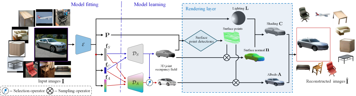
In this work, a generic object is described by three disentangled latent parameters: category, shape and albedo. Through two deep networks, these parameters can be decoded into the D shape and albedo respectively. To have an end-to-end trainable framework, we estimate these parameters along with the lighting and camera projection, via an encoder network, i.e., the fitting module of our model. Three networks work jointly for the objective of reconstructing the input image of generic objects, by incorporating a physics-based rendering layer, as in Fig. 2.
Formally, given a training set of images of multiple categories, our objective is to learn i) an encoder : that outputs the projection , lighting parameter , category code , shape code , and albedo code , ii) a shape decoder that decodes parameters to a D geometry , represented by an occupancy field, and iii) an albedo decoder that decodes parameters into a color field , with the goal that the reconstructed image by these components () can well approximate the input. This objective can be mathematically presented as:
| (1) |
where is the reconstructed image, and is the rendering function.
3.2 Category-adaptive D Joint Occupancy Fields
Unlike D, the community has not yet agreed on a D representation both memory efficient and inferable from data. Recently, implicit representations gain popularity as their continuous functions offer high-fidelity surface. Motivated by this, we propose a D joint occupancy fields (JOF) representation to simultaneously model shape and albedo with unsupervised segmentation, offering part-level correspondence for D shapes, as in Fig. 3. JOF has three novel designs over prior implicit representations [7, 33, 37, 36, 6]: 1) we extend the idea of unsupervised segmentation [6] from shape to albedo, 2) we integrate shape segmentation into albedo decoder, guiding segmentation by both geometry and appearance cues, and 3) we condition JOF on the category to model multiple categories.
Category Code. Unlike prior implicit representations, we introduce a category code as the additional input to the shape and albedo decoders. In training, is supervised by a cross-entropy loss using the class label of each image. In the context of modeling shape deformation of multiple categories, using enables decoders to focus on modeling intra-class deformations via . Further, the embedding may generalize to unseen categories too.
Shape Component. As adopted from [7, 33, 37], each shape is represented by a function, implemented as a decoder network, : , which inputs a D location , category code , shape codes and outputs its probability of occupancy . One appealing property is that the surface normal can be computed by the spatial derivative via back-propagation through the network, which is helpful for subsequent tasks such as rendering.
To offer unsupervised part segmentation, we adopt BAE-NET [6] as the architecture of . It is composed of fully connected layers and the final layer is a branched layer that gives the occupancy value for each of branchs, denoted by in Fig. 3 (a). Finally, a max pooling on the branch outputs the result of the final occupancy.
Albedo Component. Albedo component assigns each vertex on the D surface a RGB albedo. One may use a combination of category and albedo codes to represent a colored shape, i.e., . However, it puts a redundant burden to to encode the object geometry, e.g., the position of the tire, and body of a car. Hence, we also feed the shape code as an additional input to the albedo decoder, i.e., : (Fig. 3(b)).
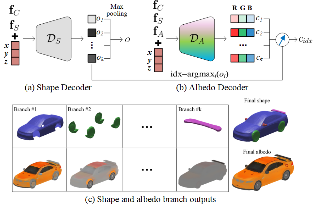
Inspired by the design of , we propose to estimate the albedo for branches . For each , the final albedo is , where is the index of segment where belongs to (Fig. 3(c)). This novel design integrates shape segmentation into albedo learning, benefiting both segmentation and reconstruction (Tab. 4). The key motivation is that, different parts of an object often differ in shape and/or albedo, and thus both shall guide the segmentation.
3.3 Physics-based Rendering
To render an image ( pixels) from shape, albedo, as well as lighting parameters and projection , we first find a set of D surface points corresponding to the D pixel. Then the RGB color of each pixel is computed via a lighting model using lighting and decoder outputs.
Camera Model. We assume a full perspective camera model. Any spatial points in the world space can be projected to camera space by a multiplication between a full perspective projection matrix and its homogeneous coordinate: , , where is the depth value of image coordinate . Essentially, can be extended to a matrix. By an abuse of notation in homogeneous coordinates, relation between D points and its camera space projection can be written as:
| (2) |
Surface Point Detection. To render a D image, for each ray from the camera to the pixel , we select one “surface point”. Here, a surface point is defined as the first interior point (), or the exterior point with the largest in case the ray doesn’t hit the object. For efficient training, instead of finding exact surface points, we approximate them via Linear or Linear-Binary search. Intuitively, with the distance margin error of , in Linear search, along each ray we evaluate for all spatial point candidates with a step size of . In Linear-Binary search, after the first interior point is found, as is a continuous function, a Binary search can be used to better approximate the surface point. With the same computational budget, Linear-Binary search leads to better approximation of surface points, hence higher rendering quality. The search algorithm is detailed in the supplementary material (Supp.).
Image Formation. We assume purely Lambertian surface reflectance and distant low-frequency illumination. Thus, the incoming radiance can be approximated via Spherical Harmonics (SH) basis functions , and controlled by coefficients . At the pixel with corresponding surface point , the image color is computed as a product of albedo and shading :
| (3) |
where is the surface normal direction at , -normalized by function . We use SH bands, which leads to coefficients for each color channel.
3.4 Semi-Supervised Model Learning
While our model is designed to learn from real-world images, we benefit from pre-training shape and albedo with CAD models, given inherent ambiguity in inverse tasks. We first describe learning from images self-supervisedly, and then pre-training from CAD models with supervision.
3.4.1 Self-supervised Joint Modeling and Fitting
Given a set of D images without ground truth D shapes, we define the loss as ( are the weights):
| (4) |
where is the photometric loss, enforces silhouette consistency, is the local feature consistency loss, and includes two regularization terms (, .
Silhouette Loss. Given the object’s silhouette , obtained by a segmentation method [43], we define the loss as:
|
|
(5) |
where are parts of the encoder that estimate , and respectively and the three inputs to are , and . With the occupancy field, the occupancy value is if , otherwise . Here, we also analyze how our silhouette loss differs from prior work. If a 3D shape is represented as a mesh, there is no gradient when comparing two binary masks, unless the predicted silhouette is expensively approximated as in Soft rasterizer [28]. If the shape is represented by a voxel, the loss can provide gradient to adjust voxel occupancy predictions, but not the object orientation [59]. Our loss can update both shape occupancy field and camera projection estimation (Eqn. 5).
Photometric Loss. To enforce similarity between our reconstruction and input, we use a loss on the foreground:
| (6) |
where is the element-wise product.
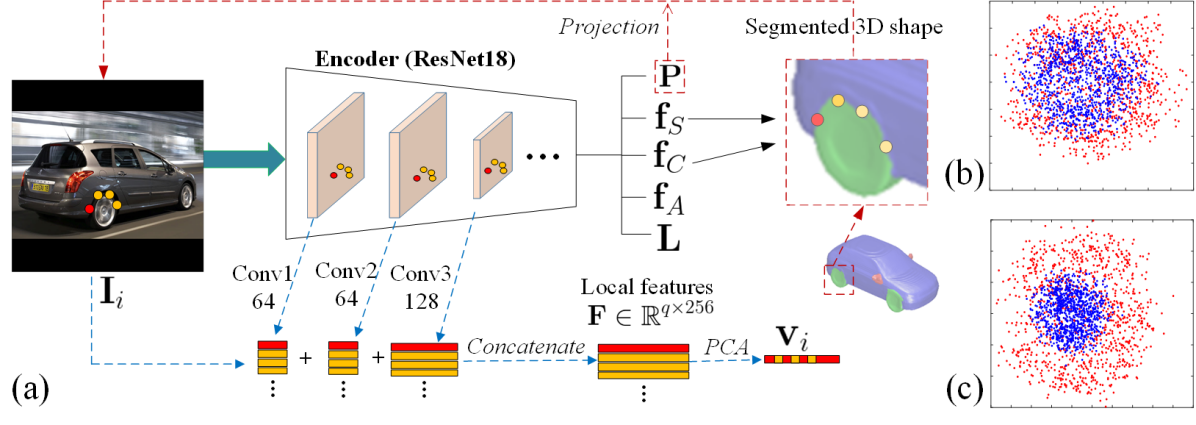
Local Feature Consistency Loss. Our decoders unsupervisedly offer part-level correspondence via learnt segmentation (Fig. 3), with which we assume that the boundary pixels of adjacent segments in one image have a similar distribution of appearance as another image of the same category. This assumption leads to a novel loss function (Fig. 4).
For one segmented D shape, we first select boundary points from all pairs of adjacent segments based on branches of , i.e., a point and its spatial neighbor shall trigger different branches. These D points are projected to the image plane via estimated . Similar to [66], we retrieve features from feature maps via the location and form the local features , where is the total feature dimension of layers. Finally, we calculate the largest eigenvector of the covariance matrix ( is the row-wise mean of ), which describes the largest feature variation of points. Despite two images of the same category may differ in colors, we assume there is similarity in their respective major variations. Thus, we define the local feature consistency loss as:
| (7) |
where is a training batch of the same category. This loss drives the semantically equivalent boundary pixels across multiple images to be projected from the same D boundary adjoining two D segments, thus improving pose and shape estimation.
Regularization Loss. We define two regularizations:
Albedo local constancy: assuming piecewise-constant albedo [24], we enforce the gradient sparsity in two directions [47]: , where represents pixel ’s neighbor pixels. Assuming that pixels with the same chromaticity (i.e., ) are more likely to have the same albedo, we set the weight , where the color is referred of the input image. We set and as in [32].
Batch-wise White Shading: Similar to [47], to prevent the network from generating arbitrary bright or dark shading, we use a batch-wise white shading constraint: , where is a red channel diffuse shading of pixel . is the total number of foreground pixels in a mini-batch. is the average shading target, which is set to . The same constraint is applied to other channels.
3.4.2 Supervised Learning with Synthetic Images
Before self-supervision, we pre-train with CAD models and synthetic data, vital for converging to faithful solutions.
Pre-training Shape and Albedo Decoder. For auto-encoding D shape and albedo, we adopt a D CNN as encoder to extract category, shape and albedo codes , , from a colored voxel. As in Fig. 5, given a dataset of CAD models, a model (with class label ) can be represented as a colored D occupancy voxel . Equivalently, it can also be represented by spatial points and their occupancy , albedo . We define the following loss:
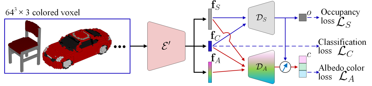
| (8) |
where , , and is cross-entropy loss for class label . Note that training is necessary to learn valid distributions of , , , although is discarded after this pre-training step.
Pre-training Image Encoder. Given a CAD model, we render multiple images of the same object with different poses and lighting, each forming a triplet of voxel, image and ground truth projection . These synthetic data can supervise the pre-training of encoder by minimizing the below, where the ground truth shape and albedo parameters are obtained by feeding voxel into ,
3.5 Implementation and Discussion
Our training process contains three steps: 1) , and are pre-trained on colored voxels and corresponding sampled point-value pairs (Eqn. 8); 2) is pre-trained with synthetic images by minimizing ; 3) and are trained using real images (Eqn. 4). We empirically found that, Step training has incremental gain when updating the shape decoder. But it significantly improves the generalization ability of our encoder on fitting model to real images. Thus, we opt to freeze the shape decoder after Step . For more details about the training setting, please refer to Supp..
One key enabler of our learning with real images is the differentiable rendering layer. For the rendering function of Eqn. 3, one can compute partial derivatives over , over since , over , , as they are the inputs of , , and over the network parameters of , . However, although the derivative over can be computed, the surface point search process is not differentiable.
4 Experimental Results
Data. We use the ShapeNet Core v1 [5] for pre-training in Steps -. Following the settings of [9, 60, 33], we use CAD models of categories and the same training/testing split. While using the same test set, we render training data ourselves, adding lighting and pose variations. We use real images of Pascal D [64] in Step training. We select categories (plane, car, chair, couch and table) which overlap with categories in synthetic data.
Metrics. We adopt standard D reconstruction metrics: F-score [21] and Chamfer- Distance (CD). Following [60], we calculate precision and recall by checking the percentage of points in prediction or ground-truth that can find the nearest neighbor from the other within a threshold . Following [33], we randomly sample points from ground-truth and estimated meshes, to compute CD.
4.1 Ablation and Analysis
| Model | CS | SU (w/o category code) | SU (w. category code) |
|---|---|---|---|
| Average CD |
Single vs. Category-specific Models. We compare two set of models on ShapeNet data: category-specific (CS) models and single universal (SU) models. CS models specialize for each particular class, which of course has better reconstruction quality (Tab. 2), and may define upper bound performance for SU. Further, we ablate the single universal model with or without category code . Clearly, the one with category code performs better, which shows that the category code does relax the burden on decoders and enable the decoders focus on the intra-class shape deformations.
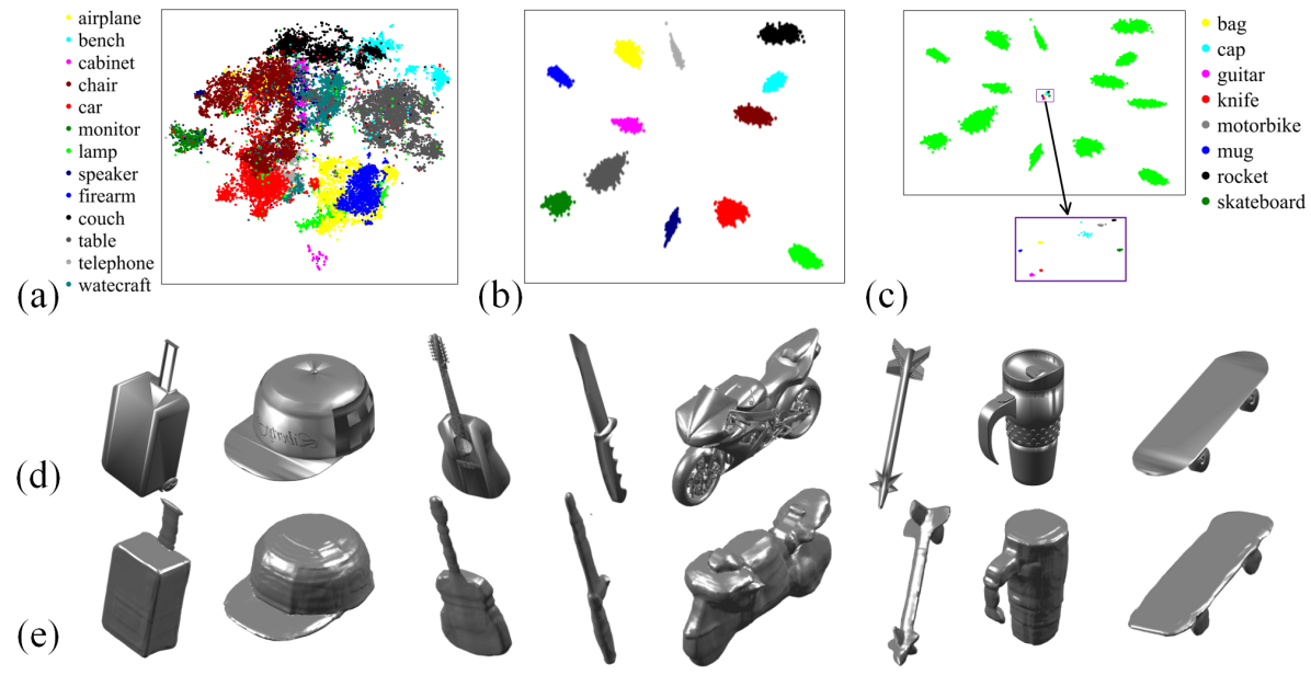
, Embedding vs. Unseen Categories. Fig. 6 (a,b) shows t-SNEs of and on categories. We observe that is more discriminative, allowing the shape decoder to capture more intra-class deformations. Further, we explore how well our shape decoder can represent the D shape of unseen classes. Thus, we randomly select samples from each of unseen ShapeNet categories. With the sampled point-value pairs of each shape, we optimize its and via back-propagation through our trained shape decoder. As in Fig. 6 (d,e), our reconstructions closely match the ground-truth. Quantitatively, we achieve a promising CD on unseen categories compare to that of unseen samples of seen categories: vs. . Additionally, we ablate our decoder with or without category code: vs. , which demonstrates enhances generalizability to unseen categories. We further visualize the estimated together with all training samples in Fig. 6 (c). As we can see, of unseen classes do not overlap with any training categories.
| w/o | w/o | w/o | Full model | |
|---|---|---|---|---|
| Azimuth angle error | ||||
| Reconstruction (CD) |
Effect of Loss Terms. Using car images of Pascal D+, we compare our full model with its partial variants, in term of pose estimation and reconstruction (Tab. 3). As the silhouette provides strong constraints on global shape and pose, without silhouette loss, performance on both metrics are severely impaired. The regularization helps to disentangle shading from albedo, which leads to better surface normal, thus better shape and pose. The local feature consistency loss helps to fine-tune the model fitting, which improves the final pose and shape estimation. Thus all the loss terms in real data training contribute to the final performance.
Effect of Training on Real Data. We evaluate D reconstructions on images from PixD and Pascal D using models obtained at different training steps. The model fine-tuned on real images (Pro. (real)) has lower Chamfer distances compare to the model learned without real images (Pro.) for every single category (Tab. 6).
4.2 Unsupervised Segmentation
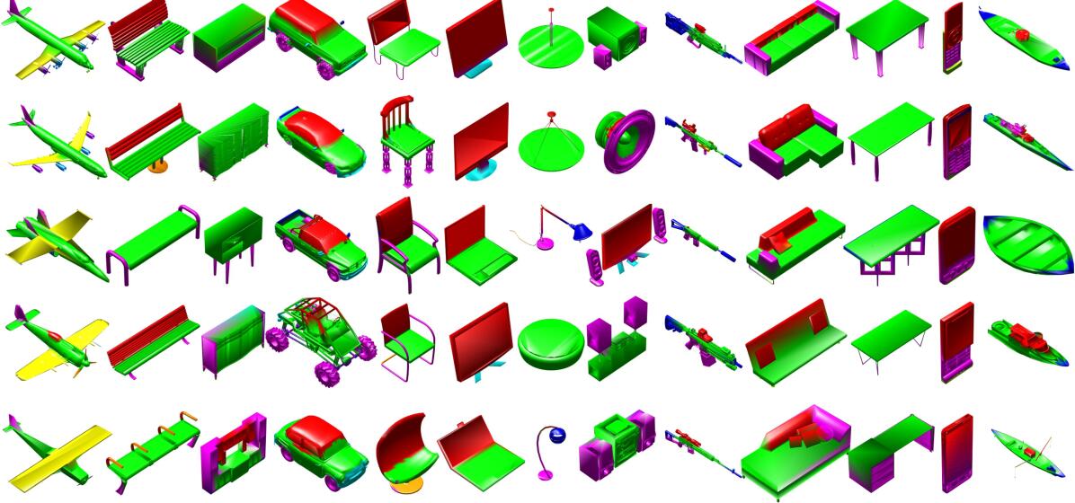
As modeling shape, albedo and co-segmentation are closely related tasks [70], joint modeling allows exploiting their correlation. Following the same setting as [6], we evaluate CS models’ co-segmentation and shape representation power on categories of airplane, chair and table. As in Tab. 4, our model achieves a higher segmentation accuracy than BAE-NET [6]. Further, we compare the ability of two models in representing D shapes. By feeding a ground-truth voxel from the testing set to the voxel encoder and then shape decoder , we evaluate how well the shape-parameter-decoded shape matches the ground-truth CAD model. The higher IoU and lower CD show that we improve both segmentation and representation accuracy. Further, Fig. 7 shows the co-segmentation across categories by our SU model. Meaningful segmentation appears both within a category and across categories. For example, chair seats, plot in green, consistently correspond to sofa seats, table tops, and bodies of airplane, car and watercraft.
|
|
|
|
|
|||||
|---|---|---|---|---|---|---|---|---|---|
| BAE-Net [6] | |||||||||
| Proposed |
4.3 Single-view D Reconstruction
| Category | Chamfer- Distance | F-score (%, ) | ||||||||||||||||||||||||||||||||||||||
|---|---|---|---|---|---|---|---|---|---|---|---|---|---|---|---|---|---|---|---|---|---|---|---|---|---|---|---|---|---|---|---|---|---|---|---|---|---|---|---|---|
|
|
|
|
|
|
|
Pro. |
|
|
|
|
|
|
Pro. | ||||||||||||||||||||||||||
| firearm | 0.115 | 0.113 | 81.35 | 79.56 | ||||||||||||||||||||||||||||||||||||
| car | 0.123 | 0.115 | 75.89 | 75.68 | ||||||||||||||||||||||||||||||||||||
| airplane | 0.104 | 0.123 | 79.15 | 77.47 | ||||||||||||||||||||||||||||||||||||
| cellphone | 0.131 | 0.130 | 77.15 | 73.91 | ||||||||||||||||||||||||||||||||||||
| bench | 0.138 | 0.137 | 66.59 | 66.15 | ||||||||||||||||||||||||||||||||||||
| watercraft | 0.151 | 0.143 | 67.30 | 63.15 | ||||||||||||||||||||||||||||||||||||
| chair | 0.184 | 0.160 | 64.72 | 63.24 | ||||||||||||||||||||||||||||||||||||
| table | 0.167 | 0.172 | 74.80 | 71.27 | ||||||||||||||||||||||||||||||||||||
| cabinet | 0.167 | 0.174 | 68.42 | 64.79 | ||||||||||||||||||||||||||||||||||||
| couch | 0.177 | 0.186 | 61.59 | 62.01 | ||||||||||||||||||||||||||||||||||||
| monitor | 0.198 | 0.185 | 63.03 | 71.45 | ||||||||||||||||||||||||||||||||||||
| speaker | 0.245 | 0.227 | 59.10 | 63.19 | ||||||||||||||||||||||||||||||||||||
| lamp | 0.209 | 0.276 | 65.11 | 63.38 | ||||||||||||||||||||||||||||||||||||
| Mean | 0.175 | 0.168 | 67.26 | 68.49 | ||||||||||||||||||||||||||||||||||||
Synthetic Images. We first evaluate D reconstruction on synthetic images. We compare with SOTA baselines that leverage various D representations: D-RN [9] (voxel), Point Set Generation (PSG) [10] (point cloud), Pixel2Mesh [60], AtlasNet [15], Front2Back [67] (mesh), and IM-SVR [7], ONet [33] (implicit field). All baselines train a single model on categories, except IM-SVR which learns models. We report the results of our SU model, trained only on synthetic images, without Step .
In general, our model is able to predict D shapes that closely resemble the ground truth (Fig. 8 (a)). Our approaches outperform baselines in most categories and achieves the best mean score, in both CD and F-score (Tab. 5). While using the same shape representation as ours, IM-SVR [7] only learns to reconstruct D shapes by minimizing the latent representation difference with ground-truth latent codes. By modeling albedo, our model benefits from learning with both supervised and self-supervised (photometric, silhouette) losses. This results in better performance both quantitatively and qualitatively.
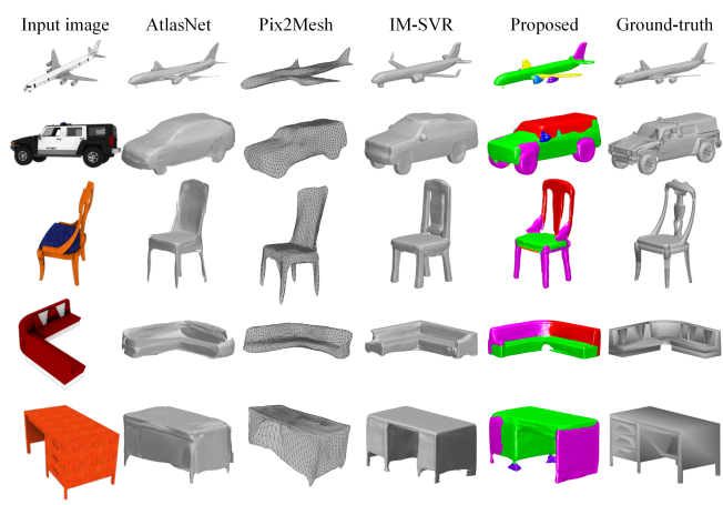
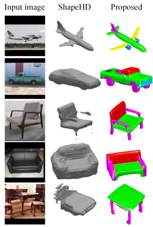
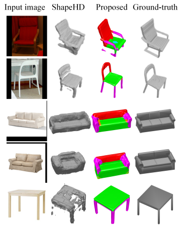
Real Images. We evaluate D reconstruction on two real image databases, Pascal D [64] and PixD [50] (overlapped categories only). We report two results of our method: a model trained with synthetic data only (Pro.) and a model fine-tuned on real images of Pascal D train subset without access to ground truth D shapes (Pro. (real)). Baselines include SOTA methods performed well on real images: D-RN [9], DRC [59], ShapeHD [63] and DAREC [39]. Among them, DRC and DAREC were trained on real images of Pascal D as they adopt a differentiable geometric consistency or domain adaptation in training. 3D-R2N2 and ShapeHD cannot be fine-tuned on real images, without albedo modeling and rendering layer.
As in Fig. 8 (b), our model infers reasonable shapes even in challenging conditions. Quantitatively, Tab. 6 shows that both proposed models outperforms other methods in Pascal D. The clear performance gap between our two models shows the importance of training on real data.
As Pascal D only has CAD models per category as ground truth shapes, ground truth labels may be inaccurate. We therefore conduct experiments on PixD database with more precise D labels. As in Tab. 6, our fine-tuned model has significantly lower CD and the best quality in Fig. 8 (c) comparing to baselines, which indicates our method can leverage real-world images without D annotations via self-supervised learning.
5 Conclusions
To better leverage real-world images in D modeling, we present a semi-supervised learning approach jointly learns the models and the fitting algorithm. While there still be a need of CAD models, our framework, with carefully-designed representation, architectures and loss functions, are able to effectively exploit real images in the training without D ground truth. Essentially, our method is applicable to any object category if both i) in-the-wild D images and ii) CAD models are available. We are interested in applying our method to a wide variety of object categories.
References
- [1] Volker Blanz, Thomas Vetter, et al. A morphable model for the synthesis of 3D faces. In Proceedings of the 26th annual conference on Computer graphics and interactive techniques, 1999.
- [2] Garrick Brazil and Xiaoming Liu. M3D-RPN: Monocular 3D region proposal network for object detection. In ICCV, 2019.
- [3] Garrick Brazil and Xiaoming Liu. Pedestrian detection with autoregressive network phases. In CVPR, 2019.
- [4] Garrick Brazil, Xi Yin, and Xiaoming Liu. Illuminating pedestrians via simultaneous detection & segmentation. In ICCV, 2017.
- [5] Angel X. Chang, Thomas Funkhouser, Leonidas Guibas, Pat Hanrahan, Qixing Huang, Zimo Li, Silvio Savarese, Manolis Savva, Shuran Song, Hao Su, Jianxiong Xiao, Li Yi, and Fisher Yu. ShapeNet: An information-rich 3D model repository. arXiv preprint arXiv:1512.03012, 2015.
- [6] Zhiqin Chen, Kangxue Yin, Matthew Fisher, Siddhartha Chaudhuri, and Hao Zhang. BAE-NET: Branched autoencoder for shape co-segmentation. In ICCV, 2019.
- [7] Zhiqin Chen and Hao Zhang. Learning implicit fields for generative shape modeling. In CVPR, 2019.
- [8] Julian Chibane, Thiemo Alldieck, and Gerard Pons-Moll. Implicit functions in feature space for 3D shape reconstruction and completion. In CVPR, 2020.
- [9] Christopher B Choy, Danfei Xu, JunYoung Gwak, Kevin Chen, and Silvio Savarese. 3D-R2N2: A unified approach for single and multi-view 3D object reconstruction. In ECCV, 2016.
- [10] Haoqiang Fan, Hao Su, and Leonidas J Guibas. A point set generation network for 3D object reconstruction from a single image. In CVPR, 2017.
- [11] Yao Feng, Fan Wu, Xiaohu Shao, Yanfeng Wang, and Xi Zhou. Joint 3D face reconstruction and dense alignment with position map regression network. In ECCV, 2018.
- [12] Kyle Genova, Forrester Cole, Avneesh Sud, Aaron Sarna, and Thomas Funkhouser. Local deep implicit functions for 3D shape. In CVPR, 2020.
- [13] Justin Johnson Georgia Gkioxari, Jitendra Malik. Mesh R-CNN. In ICCV, 2019.
- [14] Shubham Goel, Angjoo Kanazawa, and Jitendra Malik. Shape and viewpoint without keypoints. In ECCV, 2020.
- [15] Thibault Groueix, Matthew Fisher, Vladimir G Kim, Bryan C Russell, and Mathieu Aubry. AtlasNet: A papier-mâché approach to learning 3D surface generation. In CVPR, 2018.
- [16] Qixing Huang, Vladlen Koltun, and Leonidas Guibas. Joint shape segmentation with linear programming. In TOG, 2011.
- [17] Yue Jiang, Dantong Ji, Zhizhong Han, and Matthias Zwicker. SDFDiff: Differentiable rendering of signed distance fields for 3D shape optimization. In CVPR, 2020.
- [18] Angjoo Kanazawa, Shubham Tulsiani, Alexei A Efros, and Jitendra Malik. Learning category-specific mesh reconstruction from image collections. In ECCV, 2018.
- [19] Abhishek Kar, Shubham Tulsiani, Joao Carreira, and Jitendra Malik. Category-specific object reconstruction from a single image. In CVPR, 2015.
- [20] Hiroharu Kato, Yoshitaka Ushiku, and Tatsuya Harada. Neural 3D mesh renderer. In CVPR, 2018.
- [21] Arno Knapitsch, Jaesik Park, Qian-Yi Zhou, and Vladlen Koltun. Tanks and temples: Benchmarking large-scale scene reconstruction. TOG, 2017.
- [22] Nilesh Kulkarni, Abhinav Gupta, David F Fouhey, and Shubham Tulsiani. Articulation-aware canonical surface mapping. In CVPR, 2020.
- [23] Nilesh Kulkarni, Abhinav Gupta, and Shubham Tulsiani. Canonical surface mapping via geometric cycle consistency. In ICCV, 2019.
- [24] Edwin H Land and John J McCann. Lightness and retinex theory. Josa, 1971.
- [25] Xueting Li, Sifei Liu, Kihwan Kim, Shalini De Mello, Varun Jampani, Ming-Hsuan Yang, and Jan Kautz. Self-supervised single-view 3D reconstruction via semantic consistency. In ECCV, 2020.
- [26] Feng Liu and Xiaoming Liu. Learning implicit functions for topology-varying dense 3D shape correspondence. In NeurIPS, 2020.
- [27] Feng Liu, Luan Tran, and Xiaoming Liu. 3D face modeling from diverse raw scan data. In ICCV, 2019.
- [28] Shichen Liu, Weikai Chen, Tianye Li, and Hao Li. Soft Rasterizer: Differentiable rendering for unsupervised single-view mesh reconstruction. In ICCV, 2019.
- [29] Shichen Liu, Shunsuke Saito, Weikai Chen, and Hao Li. Learning to infer implicit surfaces without 3D supervision. In NeurIPS, 2019.
- [30] Shaohui Liu, Yinda Zhang, Songyou Peng, Boxin Shi, Marc Pollefeys, and Zhaopeng Cui. DIST: Rendering deep implicit signed distance function with differentiable sphere tracing. In CVPR, 2020.
- [31] Matthew Loper, Naureen Mahmood, Javier Romero, Gerard Pons-Moll, and Michael J Black. SMPL: A skinned multi-person linear model. TOG, 2015.
- [32] Abhimitra Meka, Michael Zollhöfer, Christian Richardt, and Christian Theobalt. Live intrinsic video. TOG, 2016.
- [33] Lars Mescheder, Michael Oechsle, Michael Niemeyer, Sebastian Nowozin, and Andreas Geiger. Occupancy networks: Learning 3D reconstruction in function space. In CVPR, 2019.
- [34] Ben Mildenhall, Pratul P Srinivasan, Matthew Tancik, Jonathan T Barron, Ravi Ramamoorthi, and Ren Ng. NeRF: Representing scenes as neural radiance fields for view synthesis. In ECCV, 2020.
- [35] Michael Niemeyer, Lars Mescheder, Michael Oechsle, and Andreas Geiger. Differentiable volumetric rendering: Learning implicit 3D representations without 3D supervision. In CVPR, 2020.
- [36] Michael Oechsle, Lars Mescheder, Michael Niemeyer, Thilo Strauss, and Andreas Geiger. Texture fields: Learning texture representations in function space. In ICCV, 2019.
- [37] Jeong Joon Park, Peter Florence, Julian Straub, Richard Newcombe, and Steven Lovegrove. DeepSDF: Learning continuous signed distance functions for shape representation. In CVPR, 2019.
- [38] Songyou Peng, Michael Niemeyer, Lars Mescheder, Marc Pollefeys, and Andreas Geiger. Convolutional occupancy networks. In ECCV, 2020.
- [39] Pedro O Pinheiro, Negar Rostamzadeh, and Sungjin Ahn. Domain-adaptive single-view 3D reconstruction. In ICCV, 2019.
- [40] Stylianos Ploumpis, Haoyang Wang, Nick Pears, William AP Smith, and Stefanos Zafeiriou. Combining 3D morphable models: A large scale face-and-head model. In CVPR, 2019.
- [41] Charles R Qi, Hao Su, Kaichun Mo, and Leonidas J Guibas. Pointnet: Deep learning on point sets for 3D classification and segmentation. In CVPR, 2017.
- [42] Charles Ruizhongtai Qi, Li Yi, Hao Su, and Leonidas J Guibas. Pointnet++: Deep hierarchical feature learning on point sets in a metric space. In NeurIPS, 2017.
- [43] Xuebin Qin, Zichen Zhang, Chenyang Huang, Masood Dehghan, Osmar R Zaiane, and Martin Jagersand. U2-Net: Going deeper with nested U-structure for salient object detection. Pattern Recognition, 106:107404, 2020.
- [44] Olga Russakovsky, Jia Deng, Hao Su, Jonathan Krause, Sanjeev Satheesh, Sean Ma, Zhiheng Huang, Andrej Karpathy, Aditya Khosla, Michael Bernstein, et al. Imagenet large scale visual recognition challenge. IJCV, 2015.
- [45] Shunsuke Saito, Zeng Huang, Ryota Natsume, Shigeo Morishima, Angjoo Kanazawa, and Hao Li. PIFu: Pixel-aligned implicit function for high-resolution clothed human digitization. In ICCV, 2019.
- [46] Zhenyu Shu, Chengwu Qi, Shiqing Xin, Chao Hu, Li Wang, Yu Zhang, and Ligang Liu. Unsupervised 3D shape segmentation and co-segmentation via deep learning. CAGD, 2016.
- [47] Zhixin Shu, Ersin Yumer, Sunil Hadap, Kalyan Sunkavalli, Eli Shechtman, and Dimitris Samaras. Neural face editing with intrinsic image disentangling. In CVPR, 2017.
- [48] Oana Sidi, Oliver van Kaick, Yanir Kleiman, Hao Zhang, and Daniel Cohen-Or. Unsupervised co-segmentation of a set of shapes via descriptor-space spectral clustering. TOG, 2011.
- [49] Vincent Sitzmann, Michael Zollhöfer, and Gordon Wetzstein. Scene representation networks: Continuous 3D-structure-aware neural scene representations. In NeurIPS, 2019.
- [50] Xingyuan Sun, Jiajun Wu, Xiuming Zhang, Zhoutong Zhang, Chengkai Zhang, Tianfan Xue, Joshua B Tenenbaum, and William T Freeman. Pix3D: Dataset and methods for single-image 3D shape modeling. In CVPR, 2018.
- [51] Luan Tran, Feng Liu, and Xiaoming Liu. Towards high-fidelity nonlinear 3D face morphable model. In CVPR, 2019.
- [52] Luan Tran and Xiaoming Liu. Nonlinear 3D face morphable model. In CVPR, 2018.
- [53] Luan Tran and Xiaoming Liu. On learning 3D face morphable model from in-the-wild images. TPAMI, 2019.
- [54] Luan Tran, Xi Yin, and Xiaoming Liu. Disentangled representation learning GAN for pose-invariant face recognition. In CVPR, 2017.
- [55] Luan Tran, Xi Yin, and Xiaoming Liu. Representation learning by rotating your faces. TPAMI, 2018.
- [56] Edgar Tretschk, Ayush Tewari, Vladislav Golyanik, Michael Zollhöfer, Carsten Stoll, and Christian Theobalt. PatchNets: Patch-based generalizable deep implicit 3D shape representations. In ECCV, 2020.
- [57] Shubham Tulsiani, Abhishek Kar, Joao Carreira, and Jitendra Malik. Learning category-specific deformable 3D models for object reconstruction. TPAMI, 2016.
- [58] Shubham Tulsiani, Hao Su, Leonidas J Guibas, Alexei A Efros, and Jitendra Malik. Learning shape abstractions by assembling volumetric primitives. In CVPR, 2017.
- [59] Shubham Tulsiani, Tinghui Zhou, Alexei A Efros, and Jitendra Malik. Multi-view supervision for single-view reconstruction via differentiable ray consistency. In CVPR, 2017.
- [60] Nanyang Wang, Yinda Zhang, Zhuwen Li, Yanwei Fu, Wei Liu, and Yu-Gang Jiang. Pixel2Mesh: Generating 3D mesh models from single RGB images. In ECCV, 2018.
- [61] Chao Wen, Yinda Zhang, Zhuwen Li, and Yanwei Fu. Pixel2Mesh++: multi-view 3D mesh generation via deformation. In ICCV, 2019.
- [62] Jiajun Wu, Yifan Wang, Tianfan Xue, Xingyuan Sun, Bill Freeman, and Josh Tenenbaum. MarrNet: 3D shape reconstruction via 2.5D sketches. In NeurIPS, 2017.
- [63] Jiajun Wu, Chengkai Zhang, Xiuming Zhang, Zhoutong Zhang, William T Freeman, and Joshua B Tenenbaum. Learning shape priors for single-view 3D completion and reconstruction. In ECCV, 2018.
- [64] Yu Xiang, Roozbeh Mottaghi, and Silvio Savarese. Beyond pascal: A benchmark for 3D object detection in the wild. In WACV, 2014.
- [65] Kai Xu, Honghua Li, Hao Zhang, Daniel Cohen-Or, Yueshan Xiong, and Zhi-Quan Cheng. Style-content separation by anisotropic part scales. TOG, 2010.
- [66] Qiangeng Xu, Weiyue Wang, Duygu Ceylan, Radomir Mech, and Ulrich Neumann. DISN: Deep implicit surface network for high-quality single-view 3D reconstruction. In NeurIPS, 2019.
- [67] Yuan Yao, Nico Schertler, Enrique Rosales, Helge Rhodin, Leonid Sigal, and Alla Sheffer. Front2Back: Single view 3D shape reconstruction via front to back prediction. In CVPR, 2020.
- [68] Li Yi, Haibin Huang, Difan Liu, Evangelos Kalogerakis, Hao Su, and Leonidas Guibas. Deep part induction from articulated object pairs. In SIGGRAPH Asia 2018 Technical Papers, 2018.
- [69] Li Yi, Vladimir G Kim, Duygu Ceylan, I Shen, Mengyan Yan, Hao Su, Cewu Lu, Qixing Huang, Alla Sheffer, Leonidas Guibas, et al. A scalable active framework for region annotation in 3D shape collections. TOG, 2016.
- [70] Amir R. Zamir, Alexander Sax, William B. Shen, Leonidas J. Guibas, Jitendra Malik, and Silvio Savarese. Taskonomy: Disentangling task transfer learning. In CVPR, 2018.
- [71] Xiuming Zhang, Zhoutong Zhang, Chengkai Zhang, Josh Tenenbaum, Bill Freeman, and Jiajun Wu. Learning to reconstruct shapes from unseen classes. In NeurIPS, 2018.
- [72] Xiangyu Zhu, Zhen Lei, Xiaoming Liu, Hailin Shi, and Stan Z Li. Face alignment across large poses: A 3D solution. In CVPR, 2016.