Fully (GRADCURL)-nonconforming finite element method for the singularly perturbed quad-curl problem on cubical meshes
Abstract.
In this paper, we develop two fully nonconforming (both -nonconforming and -nonconforming) finite elements on cubical meshes which can fit into the Stokes complex. The newly proposed elements have 24 and 36 degrees of freedom, respectively. Different from the fully -nonconforming tetrahedral finite elements in [9], the elements in this paper lead to a robust finite element method to solve the singularly perturbed quad-curl problem. To confirm this, we prove the optimal convergence of order for a fixed parameter and the uniform convergence of order for any value of . Some numerical examples are used to verify the correctness of the theoretical analysis.
Key words and phrases:
nonconforming finite elements, singularly perturbed quad-curl problem, cubical elements2000 Mathematics Subject Classification:
65N30 and 35Q60 and 65N15 and 35B451. Introduction
The quad-curl equation appears in various models, such as the inverse electromagnetic scattering theory [3, 13, 16], couple stress theory in linear elasticity [11, 14], and magnetohydrodynamics [24]. The corresponding quad-curl eigenvalue problem plays a fundamental role in the analysis and computation of the electromagnetic interior transmission eigenvalues [15]. In this paper, we consider the following quad-curl singular perturbation problem on a bounded polyhedral domain : find such that
| (1.1) | ||||
Here , and are constants of moderate size, is a constant that can approach 0, and is the unit outward normal vector to .
Standard conforming finite element methods to solve problem (1.1) require function spaces to be subspaces of , see Section 2 for its precise definition. Some (gradcurl)-conforming finite elements have been constructed in the past years. So far, the construction in 2 dimensions(2D) is relatively complete [20, 7, 18], however, that is not the case for 3 dimensions (3D). In [22], one of the authors and Z. Zhang developed a tetrahedral -conforming element, which has degrees of freedom (DOFs) on each element. To reduce the number of DOFs, they, together with their collaborators, enriched the shape function space on each tetrahedron with piecewise-polynomial bubbles [8], and the resulting element has only 18 DOFs. However, it is challenging to extend the idea of enriching bubbles to cubical element. The only grad curl-conforming element on cubical meshes constructed in [17] has DOFs on each cube.
Therefore, we resort to nonconforming elements to reduce the number of DOFs. On tetrahedral meshes, Zheng et al. constructed the first nonconforming finite element in [24], which has DOFs on each element. Recently, Huang [9] proposed a nonconforming finite element Stokes complex which includes two -nonconforming finite elements: one coincides with the element in [24] and the other one has only 14 DOFs. However, the convergence rates of the two nonconforming finite elements in [9, 24] will deteriorate when in problem (1.1). Hence, Huang and Zhang in [10] developed two families of -nonconforming but (curl)-conforming finite elements on tetrahedral meshes, which can solve problem (1.1) when tends to zero, see also [19]. On cubical meshes, one of the authors and her collaborators proposed a family of nonconforming finite elements with at least DOFs in [21]. This family is also (curl)-conforming, and hence can solve problem (1.1) as vanishes. To further reduce the number of DOFs, in this paper, we will construct both -nonconforming and -nonconforming finite elements. Different with the tetrahedral elements, the fully nonconforming elements that we will construct still work for problem (1.1) when .
To this end, we consider the following Stokes complex:
| (1.2) |
We will develop the fully -nonconforming elements by constructing a discrete nonconforming Stokes complex on cubical meshes:
| (1.3) |
where , , , and are conforming or nonconforming finite element spaces for , , , and , respectively. To make the number of DOFs as minimal as possible, we use the -th order serendipity finite element space with for . We choose the nonconforming Stokes pair developed in [23] for and . Then the -nonconforming finite element space is obtained as the gradient of and a complementary part whose falls into . To be precise, the shape function space of is
where and are shape function spaces of and and is the Poincaré operator with the precise definition given in Sections 3. The DOFs of can be obtained from the DOFs of and . By taking , we will get two versions of . The number of DOFs on each element is 24 for and 36 for . By constructing in this way, we can show that the complex (1.3) is exact on contractible domains.
Based on the newly proposed and , we develop a robust mixed finite element method for solving the quad-curl singular perturbation problem (1.1). The wellposedness of the numerical scheme holds by proving the discrete Poincaré inequality, the discrete inf-sup condition, and the coercivity condition. Moreover, we prove a special property of functions in :
| (1.4) |
where is defined in Section 4. With the interpolation results, projection error estimates, and property (1.4), we obtain an optimal convergence order for any fixed . As approaches , the right-hand side of the optimal estimate will blow up, which makes the estimate useless. Therefore, we also provide a uniform convergence order for any value of in the sense of the energy norm. We note that the optimal estimate for a moderate can be obtained without using property (1.4), while the uniform estimate can not. The fully nonconforming finite elements on tetrahedral meshes [9] do not possess this property, which is the reason that those elements can not work for the quad-curl singular perturbation problem.
The rest of the paper is organized as follows. In section 2 we list some notation that will be used throughout the paper. In section 3 we define the fully -nonconforming finite element on a cube and estimate the interpolation errors. Nonconforming and exact finite element complexes are constructed in section 4. In section 5 we use our proposed elements to solve the quad-curl singularly perturbed problem and obtain the optimal convergence order of the energy error for any fixed . In section 6 we provide a uniform error estimate with respect to . In section 7, numerical examples are shown to verify the correctness and efficiency of our method. Finally, some concluding remarks are given in section 8.
2. Notation
We assume that is a contractible Lipschitz domain throughout the paper. We adopt conventional notation for Sobolev spaces such as or on a sub-domain furnished with the norm and the semi-norm . In the case of , we use notation or for spaces or . The norm and semi-norm are and , respectively. In the case of , the space coincides with which is equipped with the inner product and the norm . When , we drop the subscript .
In addition to the standard Sobolev spaces, we also define
For a subdomain , we use , or simply when there is no possible confusion, to denote the space of polynomials with degree at most on . We denote the space of polynomials in three variables whose maximum degrees are in , in , and in , respectively.
For a scalar function space , we use or to denote the .
Let be a partition of the domain consisting of shape-regular cuboids. For , we denote as the diameter of and as the mesh size of . Denote by , , and the sets of vertices, edges, and faces in the partition, and , , and the sets of interior vertices, edges, and faces. We also denote by , , and the sets of vertices, edges, and faces related to the element . We use and to denote the unit tangential vector and the unit normal vector to and , respectively. Suppose . For a function defined on , we define to be the jump across . When , .
We use to denote a generic positive constant that is independent of .
3. The H(gradcurl)-Nonconforming Finite Elements
In this section, we will construct -nonconforming finite elements on cubical meshes. To this end, recall the Poincaré operator [4] defined by
The Poincaré operator satisfies
| (3.1) | |||
| (3.2) |
where and . It holds
| (3.3) |
For each element , we define the following shape function space:
| (3.4) |
where
| (3.5) |
and for , the shape function space contains all polynomials of superlinear degree at most . The superlinear degree of a polynomial is the degree with ignoring variables that enter linearly. For example, is a polynomial with superlinear degree . To be specific, the space is spanned by the monomials in and
We have and . The space is the same as the space defined in [23] and .
The right-hand side of (3.4) is a direct sum. In fact, if , then and . According to (3.2), we have . From the definition of , we have and
We define the following DOFs for :
| (3.6) | ||||
| (3.7) |
Remark 3.1.
The DOFs can be equivalently defined as
| (3.8) | |||
| (3.9) |
where are two unit vectors parallel to the two non-colinear edges in face .
Lemma 3.1.
The DOFs and are well-defined for .
Proof.
The boundedness of the DOFs is trivial. To prove the boundedness of DOFs , we apply a similar idea to the proof of [12, Lemma 5.38]. For an edge , is the face containing the edge on its boundary. Given a polynomial , we extend it by 0 to a function on (still denoted by ). Such a function is in with and . Suppose is an element containing the face on its boundary, we have
Proof.
First of all, the number of DOFs (3.7)-(3.6) is which is same as the dimension of . Then it suffices to show that if all the DOFs (3.7)-(3.6) vanish on a function with and , then .
For each , by the integration by parts on face , we have
| (3.10) |
which together with vanishing DOFs in (3.7), we obtain
| (3.11) |
By (3.1) and the definition of , we have .
The unisolvence of the DOFs for [23] leads to , which implies . Then . Using the DOFs (3.6), we can obtain , then we can choose satisfying for each . Since the superlinear degree of is no more than , we can get .
For the reference element , we denote the DOFs for by
We relate the shape function on and on by
| (3.12) |
where is a affine mapping from reference element to an element . For technical reasons, we assume the elements in have all edges parallel to the coordinates axes, then is a diagonal matrix.
For any , we define an interpolation operator by
| (3.13) |
Similarly, we can define . The following lemma establishes the relationship between the interpolation on and the interpolation on .
Lemma 3.3.
Suppose that is well defined. Then under the transformation (3.12), we have
Proof.
The interpolations and are defined by DOFs and , respectively. Under the transformation (3.12) , each DOF in is a constant multiple of the corresponding DOF in . For example
where we have used the facts that is a diagonal matrix and .
Therefore the two interpolations are identical according to [2, Proposition 3.4.7].
With the help of Lemma 3.3, we can show that the interpolation operator has the following approximation property.
4. Nonconforming finite element Stokes complexes
4.1. A finite element de Rham complex on cubical meshes
In this section, we present the precise definition of each space involved in the complex (1.3).
Space
This is the -conforming serendipity finite element space [1]. The shape function space is and the DOFs for are
-
•
function values at all vertices ,
-
•
moments at all edges .
The above DOFs lead to the canonical interpolation : with .
Space
The space is defined by
We define a global interpolation operator element-wisely by
Space
For , we use the -nonconforming finite element space in [23], which was constructed for the Darcy-Stokes-Brinkman problem. The shape function space is defined by (3.5).
The DOFs for are
-
•
moments at all faces .
Applying the above DOFs, we can define an interpolation , whose restriction on is denoted as .
Space
The shape function space of on is . For , the DOFs are
-
•
moments at all elements .
The above DOFs lead to the canonical interpolation : , whose restriction on is denoted as .
We summarize the interpolations defined by the DOFs in the following diagram.
| (4.1) |
Lemma 4.1.
The interpolations in the diagram (4.1) commute with the differential operators, i.e.,
Proof.
It is straightforward to prove the lemma by following the argument in the proof of [7, Lemma 4.5].
Lemma 4.2.
The complex (1.3) is exact when is contractible.
Proof.
To prove the complex is exact, we shall show that the complex is exact at each space. We start with . We suppose and , and we show that there exists a such that . Since , we can write with for any . Suppose is a common face of . Restricted on , the polynomials and are in (the counterpart of in 2D). The DOFs for any and yield on each , and hence for some on , . Restricting to four vertices of leads to , and hence on . We then pick a such that . Therefore, we can glue together all for to get a function . The exactness at follows from the exactness at the same position of smooth Stokes complex and the commutativity of interpolations and (Lemma 4.1)[21].
Finally, we prove the exactness at by a dimension count. Let be the number of elements in . Then
which together with Euler’s formula leads to
Define
Proceeding as the proof of Lemma 4.2, we can prove the following exactness of the complex with vanishing boundary DOFs.
Lemma 4.3.
The complex
| (4.2) |
is exact when is contractible.
5. Application of the Nonconforming Elements to the Model Problem
We define with vanishing boundary conditions:
To deal with the divergence-free condition, we introduce a Lagrange multiplier . The mixed variational formulation is to find such that
| (5.1) |
with and .
Taking in (5.1) and using the vanishing boundary condition of , we can obtain that .
The nonconforming finite element method for (5.1) seeks such that
| (5.2) |
where . Define
and
where and means taking element by element. To show the well-posedness of numerical scheme (5.2), we will first prove the discrete Poincaré inequality for functions in . To this end, we follow the idea in [9] and define the interpolation for by
| (5.3) |
Then we have [12, Theoreoms 6.7, 6.3]
| (5.4) |
Proceeding as in the proof of [9, Lemma 4.2], it holds that
| (5.5) |
Define
Then is determined by
For , since is single-valued for and , , and hence is well-defined.
For simplicity, we denote as when .
Now we are ready to prove the discrete Poincaré inequality.
Lemma 5.1.
The following discrete Poincaré inequality holds
| (5.6) |
Proof.
According to the discrete Helmholtz decomposition [12], it follows that
| (5.7) |
with and . By (5.7) and the discrete Poincaré inequality for , we can arrive at
which implies
Therefore, we have
Then (5.6) follows immediately from (5.4), (5.5), and the inverse inequality.
Remark 5.1.
Different with the proof of [9, lemma 4.3], our method does not require the existence of bounded commuting projection operators.
We are now in a position to state the wellposedness of the numerical scheme. The finite element spaces and satisfy:
-
•
the inf-sup condition
(5.8) - •
Then the finite element scheme is well-posed.
Theorem 5.1.
Proof.
Define
| (5.11) |
Then estimate (5.10) follows from [21, Theorem 3.3]. From integration by parts and the fact that , we get
To estimate the consistency error , we need the following lemma, which is the key for the element working for problem (1.1) with small .
Lemma 5.2.
For any and , we have
| (5.12) |
where is the unit outward normal vector to .
Proof.
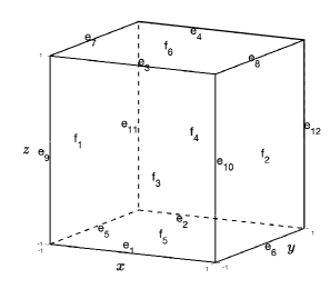
We will prove the lemma only for , and the lemma for can be obtained similarly. For an element , we sort the edges and faces as in Figure 5.1. Then we can rewrite and as follows,
| (5.13) | ||||
| (5.14) | ||||
where , and are the corresponding dual basis functions of on and , and is the dual basis function of on .
We will show that for and for and . The functions , , and are the corresponding basis functions on the reference element . Here we present only , and :
Then
with . After a direct calculation, we derive . Similarly,
with .
Theorem 5.2.
Proof.
We use the right-hand side of (5.10) to estimate (5.15). Due to and the error estimates of the interpolation (3.14)–(3.15), we have
| (5.16) |
To estimate the consistency error term , we estimate each term in . Firstly,
| (5.17) |
Here and hereafter is unit outward normal vector to and is the projection to . The projection satisfies
| (5.18) |
To estimate the second term of the consistency error, we apply Lemma 5.2 to get
| (5.19) |
To estimate the last term of the consistency error, we follow an analogous idea in [9] and have
| (5.20) |
6. Uniform Error Estimates
In Theorem 5.2, we assume are bounded. However, we can not expect that the bound of is independent of . To reveal this, we consider the following second-order problem:
| (6.1) | ||||
We assume satisfies the following regularity estimate
| (6.2) |
Without loss of generality, we assume in this section. Let be the solution of problem (1.1). According to the proof of [10, Lemma 3.1 – 3.2], we can prove
| (6.3) | ||||
| (6.4) |
From (6.4), we can see the bound of will blow up as approaches 0, in which case the estimate 5.2 would fail. In this section, we will provide a uniform error estimate with respect to .
Subtracting (6.1) from (1.1) leads to
For , by using integration by parts, we can get
| (6.5) |
Before we present the uniform error estimate, we first prove some new approximation properties of , which is based on the following boundedness of the interpolation operators and :
| (6.6) | |||
| (6.7) |
Here we have used the trace inequality [2, Theorem 1.6.6]
| (6.8) |
and the first inequality of (6.6) is a direct result of the proof of Lemma 3.1.
Lemma 6.1.
If , , there hold the following error estimates
| (6.9) | ||||
| (6.10) |
Proof.
Again, we follow the proof of [12, Theorem 5.41] and use the transformation (3.12) to have
We then apply (6.6) and [12, Theorem 5.5] to derive
Lemma 6.2.
Given , let . The projection has the following estimate:
Proof.
Theorem 6.1.
Proof.
Now we estimate the consistency error term by term. We proceed as in (5) to estimate the first term. Applying (5.18) to and Lemma 6 to , respectively, it holds that
| (6.13) |
For the last two terms of the consistency error, we have
| (6.14) |
Combining (6), (6), and (6), we can get (6.11) based on the assumption (6.2).
7. NUMERICAL EXPERIMENTS
In this section, numerical results are provided to verify the theoretical results. In this section, we assume .
Example 1.
We first consider problem (1.1) on with a smooth exact solution
The source term can be obtained by a simple calculation.
We first uniformly partition the domain into eight small cubes and then each small cube is partitioned into eight half-sized cubes to get a refined grid.
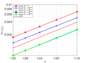
We first use the finite element spaces in discrete problem (5.2). We present and for different values of in Figure 7.1. From the result of shown in Figure 7.1(a), we can observe that the numerical results are consistent with Theorem 5.2.
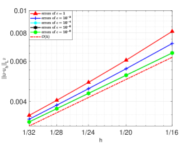
We then apply in (5.2). See Figure 7.2 for the numerical results. Again the numerical result shown in Figure 7.2(a) validate the theoretical result in Theorem 5.2.
We also observe from Figures 7.1(a) and 7.2(a) that when , and , the convergence rate of is 2. This is because the part dominates in these cases, and has convergence rate 2.
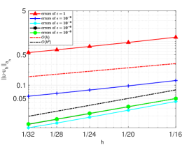
From Figures 7.1(b) and 7.2(b), we can see that the difference between the two families and is the convergence order in the sense of norm.

Example 2.
We now consider an exact solution with boundary layer. We take the source term as
with
Then according to (6.4), , which goes to 0 when approaches 0.
| order | order | order | ||||
|---|---|---|---|---|---|---|
| 1/4 | 3.231e01 | * | 3.451e+00 | * | 3.781e+00 | * |
| 1/8 | 1.623e01 | 0.99 | 1.937e+00 | 0.83 | 2.108e+00 | 0.84 |
| 1/16 | 8.261e02 | 0.97 | 1.295e+00 | 0.58 | 1.389e+00 | 0.60 |
| 1/32 | 4.168e02 | 0.99 | 9.049e01 | 0.52 | 9.628ee01 | 0.53 |
| order | order | order | ||||
|---|---|---|---|---|---|---|
| 1/4 | 3.231e01 | * | 3.451e+00 | * | 3.774e+00 | * |
| 1/8 | 1.623e01 | 0.99 | 1.937e+00 | 0.83 | 2.100e+00 | 0.85 |
| 1/16 | 8.261e02 | 0.97 | 1.295e+00 | 0.58 | 1.378e+00 | 0.61 |
| 1/32 | 4.168e02 | 0.99 | 9.049e01 | 0.52 | 9.466e01 | 0.54 |
8. Conclusion
In this paper, we constructed two fully -nonconforming finite elements on cubical meshes, which together with the Lagrange element and the nonconforming Stokes element in [23] form a nonconforming finite element Stokes complex. Moreover, we proved a special property of the proposed elements, see Lemma 5.2. With this property, we proved the optimal convergence and uniform convergence when applying the elements to solve the singularly perturbed quad-curl problem.
References
- [1] D. N. Arnold and G. Awanou. The serendipity family of finite elements. Foundations of computational mathematics, 11(3):337–344, 2011.
- [2] S. C. Brenner and L. R. Scott. The mathematical theory of finite element methods, volume 3. Springer, 2008.
- [3] F. Cakoni and H. Haddar. A variational approach for the solution of the electromagnetic interior transmission problem for anisotropic media. Inverse Problems and Imaging, 1(3):443–456, 2017.
- [4] S. H. Christiansen and K. Hu. Generalized finite element systems for smooth differential forms and Stokes’ problem. Numerische Mathematik, 140(2):327–371, 2018.
- [5] F. Demengel and G. Demengel. Functional spaces for the theory of elliptic partial differential equations. Springer, 2012.
- [6] P. Grisvard. Elliptic problems in nonsmooth domains. SIAM, 2011.
- [7] K. Hu, Q. Zhang, and Z. Zhang. Simple curl-curl-conforming finite elements in two dimensions. SIAM Journal on Scientific Computing, 42(6):A3859–A3877, 2020.
- [8] K. Hu, Q. Zhang, and Z. Zhang. A family of finite element stokes complexes in three dimensions. SIAM Journal on Numerical Analysis, 60(1):222–243, 2022.
- [9] X. Huang. Nonconforming finite element Stokes complexes in three dimensions. arXiv:2007.14068, pages 1–26, 2020.
- [10] X. Huang and C. Zhang. Robust mixed finite element methods for a quad-curl singular perturbation problem. arXiv preprint arXiv:2206.10864, 2022.
- [11] R. D. Mindlin and H. F. Tiersten. Effects of couple-stresses in linear elasticity. Archive for Rational Mechanics and Analysis, 11(1):415–448, 1962.
- [12] P. Monk. Finite Element Methods for Maxwell’s Equations. Oxford University Press, 2003.
- [13] P. Monk and J. Sun. Finite element methods for Maxwell’s transmission eigenvalues. SIAM Journal on Scientific Computing, 34(3):B247–B264, 2012.
- [14] S. K. Park and X. Gao. Variational formulation of a modified couple stress theory and its application to a simple shear problem. Zeitschrift für angewandte Mathematik und Physik, 59(5):904–917, 2008.
- [15] J. Sun. Iterative methods for transmission eigenvalues. SIAM Journal on Numerical Analysis, 49(5):1860–1874, 2011.
- [16] J. Sun. A mixed FEM for the quad-curl eigenvalue problem. Numerische Mathematik, 132(1):185–200, 2016.
- [17] L. Wang, H. Li, and Z. Zhang. )-conforming spectral element method for quad-curl problems. Computational Methods in Applied Mathematics, 21(3):661–681, 2021.
- [18] L. Wang, W. Shan, H. Li, and Z. Zhang. )-conforming quadrilateral spectral element method for quad-curl problems. Mathematical Models and Methods in Applied Sciences, 31(10):1951–1986, 2021.
- [19] B. Zhang and Z. Zhang. A new family of nonconforming elements with -continuity for the three-dimensional quad-curl problem. arXiv:2206.12056v1, 2022.
- [20] Q. Zhang, L. Wang, and Z. Zhang. )-conforming finite elements in 2 dimensions and applications to the quad-curl problem. SIAM Journal on Scientific Computing, 41(3):A1527–A1547, 2019.
- [21] Q. Zhang, M. Zhang, and Z. Zhang. Nonconforming finite elements for the brinkman and problems on cubical meshes. arXiv preprint arXiv:2206.08493v2, 2022.
- [22] Q. Zhang and Z. Zhang. A family of curl-curl conforming finite elements on tetrahedral meshes. CSIAM Transactions on Applied Mathematics, 1(4):639–663, 2020.
- [23] S. Zhang, X. Xie, and Y. Chen. Low order nonconforming rectangular finite element methods for darcy-stokes problems. Journal of Computational Mathematics, pages 400–424, 2009.
- [24] B. Zheng, Q. Hu, and J. Xu. A nonconforming finite element method for fourth order curl equations in . Mathematics of Computation, 80(276):1871–1886, 2011.