Fully-heavy tetraquark states and their evidences in the LHC observations

Searching for genuine exotic hadrons beyond the conventional quark model has been one of the most important initiatives since the establishment of the nonrelativistic constituent quark model in 1964 GellMann:1964nj ; Zweig:1981pd . Benefited from great progresses in experiment, many candidates of exotic hadrons have been found since the discovery of $X(3872)$ by Belle in 2003 Choi:2003ue . Recent reviews of the status of experimental and theoretical studies can be found in Refs. Liu:2019zoy ; Esposito:2016noz ; Olsen:2017bmm ; Lebed:2016hpi ; Chen:2016qju ; Ali:2017jda ; Guo:2017jvc . While many observed candidates have been found located in the vicinity of $S$-wave open thresholds, no signals for overall-color-singlet multiquark states have been indisputably established due to difficulties of distinguishing them from hadronic molecules Guo:2017jvc . Recently, the tetraquarks of all-heavy systems, such as $cc\bar{c}\bar{c}$ and $bb\bar{b}\bar{b}$, have received considerable attention. Since the light quark degrees of freedom cannot be exchanged between two heavy mesons at leading order, the color interactions between the heavy quarks (antiquarks) should be dominant at short distance and they may favor to form genuine color-singlet tetraquark configurations rather than loosely bound hadronic molecules. Furthermore, such exotic states may have masses and decay modes significantly different from other conventional states, thus, can be established in experiment.

Early theoretical studies of the full-heavy tetraquark states can be found in the literature Ader:1981db ; Iwasaki:1975pv ; Zouzou:1986qh ; Heller:1985cb ; Lloyd:2003yc ; Barnea:2006sd . A revival of this topic driven by the experimental progresses can be found by the intensive publications recently Wang:2017jtz ; Karliner:2016zzc ; Berezhnoy:2011xn ; Bai:2016int ; Anwar:2017toa ; Esposito:2018cwh ; Chen:2016jxd ; Wu:2016vtq ; Hughes:2017xie ; Richard:2018yrm ; Debastiani:2017msn ; Wang:2018poa ; Richard:2017vry ; Vijande:2009kj ; Deng:2020iqw ; Ohlsson ; Wang:2019rdo ; Bedolla:2019zwg ; Chen:2020lgj ; Chen:2018cqz ; Liu:2019zuc . Physicists are very concerned with the stability of the tetraquark $cc\bar{c}\bar{c}$ ($T_{(4c)}$) and $bb\bar{b}\bar{b}$ ($T_{(4b)}$) states. If the $T_{(4c)}$ or $T_{(4b)}$ states have relatively smaller masses below the thresholds of heavy charmonium or bottomonium pairs Wang:2017jtz ; Karliner:2016zzc ; Berezhnoy:2011xn ; Bai:2016int ; Anwar:2017toa ; Esposito:2018cwh ; Debastiani:2017msn ; Wang:2018poa , they may become “stable” because no direct decays into heavy quarkonium pairs through quark rearrangements would be allowed. However, some studies showed that stable bound tetraquark states made of $cc\bar{c}\bar{c}$ or $bb\bar{b}\bar{b}$ may not exist Wu:2016vtq ; Lloyd:2003yc ; Ader:1981db ; Hughes:2017xie ; Richard:2018yrm ; Richard:2017vry ; Liu:2019zuc ; Deng:2020iqw ; Wang:2019rdo ; Chen:2016jxd ; Chen:2018cqz because the the predicted masses are large enough for them to decay into heavy quarkonium pairs. Due to these very controversial issues, experimental evidence for such exotic objects would be crucial for our understanding of the underlying dynamics.

In 2020, the LHCb Collaboration reported their results on the observations of $T_{(4c)}$ states LHCexp . In the di-$J/\psi$ invariant mass spectrum, a broad structure above $J/\psi J/\psi$ threshold ranging from 6.2 to 6.8 GeV and a narrower resonance $X(6900)$ were observed with more than 5 $\sigma$ of significance level. There are also some vague structures around 7.2 GeV to be confirmed. Later in 2022, $X(6900)$ was confirmed in the same final state by both the ATLAS ATLASexp and CMS CMSexp collaborations. Some signal of $X(6900)$ was also seen in the $J/\psi\psi(2S)$ channel by the ATLAS Collaboration ATLASexp . In addition, in the lower mass region the CMS measurements show that a clear resonance $X(6600)$ together with a small shoulder structure around $6.2-6.4$ GeV lies in the di-$J/\psi$ spectrum CMSexp . These clear structures may be evidences for genuine tetraquark $T_{(4c)}$ states, they can also set up experimental constraints on theoretical models of which the successful interpretations and most importantly the early predictions should bring a lot of insights to the underlying dynamics. Stimulated by the newly observed structures in the di-$J/\psi$ invariant mass spectrum, the study of full-heavy tetraquark states has been a hot topic in the last two years Dong:2022sef ; Chen:2022mcr ; Faustov:2022mvs ; Niu:2022cug ; Wang:2022yes ; An:2022qpt ; Biloshytskyi:2022dmo ; Wang:2022jmb ; Gong:2022hgd ; Wu:2022qwd ; Zhuang:2021pci ; Yan:2021glh ; Wang:2021mma ; Majarshin:2021hex ; Wang:2021kfv ; Yang:2021hrb ; Huang:2021vtb ; Goncalves:2021ytq ; Liu:2020tqy ; Wang:2020tpt ; Wan:2020fsk ; Gong:2020bmg ; Cao:2020gul ; Guo:2020pvt ; Zhu:2020xni ; Zhang:2020xtb ; Feng:2020riv ; Ma:2020kwb ; Dong:2020nwy ; Wang:2020dlo ; Karliner:2020dta ; Wang:2020wrp ; Giron:2020wpx ; Wang:2020gmd ; Chen:2020xwe ; Wang:2020ols ; Yang:2020rih ; Niu:2022vqp ; Liang:2022rew ; Liang:2021fzr ; Dong:2021lkh ; Li:2021ygk ; Ke:2021iyh ; Yang:2020wkh ; Weng:2020jao ; Zhao:2020nwy ; Zhou:2022xpd ; Kuang:2023vac ; Zhao:2020jvl ; Becchi:2020mjz ; Becchi:2020uvq ; Chen:2022sbf .

In Refs. Liu:2019zuc ; Liu:2021rtn we adopted a nonrelativistic potential quark model (NRPQM), which is based on the Hamiltonian proposed by the Cornell model Eichten:1978tg , for the study of fully-heavy tetraquark system. The masses of the $1S$-wave fully-heavy tetraquark states were predicted there and we found that the $1S$-wave $T_{(4c)}$ masses should be above the two-charmonium thresholds within a commonly accepted parameter space Liu:2019zuc . This turns out to be consistent with the structure $X(6600)$. The predicted masses of the $2S$-wave $T_{(4c)}$ states are comparable with the narrow structure $X(6900)$. Later studies by Refs. Wang:2019rdo ; Wang:2021kfv ; Lu:2020cns ; Li:2021ygk ; Zhao:2020jvl turn out to agree with our predictions.

In this work we carry out a systematic study of the fall-apart decays of the $1S$-, $2S$- and $1P$-wave $T_{(4Q)}$ states in the NRPQM framework. The $1S$-, $2S$- and $1P$-wave $T_{(4Q)}$ ($Q=c,b$) states are calculated in the same framework. Thus, it allows us to obtain a self-consistent treatment for the mass spectrum and decay properties. We will show that some of these structures observed at LHC may arise from the $S$- and $P$-wave $T_{(4c)}$ states. To proceed, we first give a brief introduction to our model and method.

Apart from the linear confinement, Coulomb type potential, and spin-spin interaction potential for calculating the $S$-wave tetraquark states in the Hamiltonian Liu:2019zuc , we include the spin-orbit and tensor potentials here to deal with the first orbital ($1P$) excitation,

$$\begin{split}V^{LS}_{ij}=&-\frac{\alpha_{ij}}{16}\frac{{\mbox{\boldmath$\lambda$\unboldmath}}_{i}\cdot{\mbox{\boldmath$\lambda$\unboldmath}}_{j}}{r_{ij}^{3}}\bigg{(}\frac{1}{m_{i}^{2}}+\frac{1}{m_{j}^{2}}+\frac{4}{m_{i}m_{j}}\bigg{)}\bigg{\{}\mathbf{L}_{ij}\cdot(\mathbf{S}_{i}+\mathbf{S}_{j})\bigg{\}}\\ &-\frac{\alpha_{ij}}{16}\frac{{\mbox{\boldmath$\lambda$\unboldmath}}_{i}\cdot{\mbox{\boldmath$\lambda$\unboldmath}}_{j}}{r_{ij}^{3}}\bigg{(}\frac{1}{m_{i}^{2}}-\frac{1}{m_{j}^{2}}\bigg{)}\bigg{\{}\mathbf{L}_{ij}\cdot(\mathbf{S}_{i}-\mathbf{S}_{j})\bigg{\}},\end{split}$$

(1)

$$V^{T}_{ij}=-\frac{\alpha_{ij}}{4}({\mbox{\boldmath$\lambda$\unboldmath}}_{i}\cdot{\mbox{\boldmath$\lambda$\unboldmath}}_{j})\frac{1}{m_{i}m_{j}r_{ij}^{3}}\Bigg{\{}\frac{3(\mathbf{S}_{i}\cdot\mathbf{r}_{ij})(\mathbf{S}_{j}\cdot\mathbf{r}_{ij})}{r_{ij}^{2}}-\mathbf{S}_{i}\cdot\mathbf{S}_{j}\Bigg{\}},$$

(2)

where $r_{ij}\equiv|\mathbf{r}_{i}-\mathbf{r}_{j}|$ is the distance between the $i$th and $j$th quarks, $\mathbf{S}_{i}$ stands for the spin of the $i$-th quark, and $\mathbf{L}_{ij}$ stands for the relative orbital angular momentum between the $i$-th and $j$-th quark. If the interaction occurs between two quarks or antiquarks, operator $\mbox{\boldmath$\lambda$\unboldmath}_{i}\cdot\mbox{\boldmath$\lambda$\unboldmath}_{j}$ is defined as $\mbox{\boldmath$\lambda$\unboldmath}_{i}\cdot\mbox{\boldmath$\lambda$\unboldmath}_{j}\equiv\sum_{a=1}^{8}\lambda_{i}^{a}\lambda_{j}^{a}$, while if the interaction occurs between a quark and antiquark, we have $\mbox{\boldmath$\lambda$\unboldmath}_{i}\cdot\mbox{\boldmath$\lambda$\unboldmath}_{j}\equiv\sum_{a=1}^{8}-\lambda_{i}^{a}\lambda_{j}^{a*}$, where $\lambda^{a*}$ is the complex conjugate of the Gell-Mann matrix $\lambda^{a}$. The parameters $b_{ij}$ and $\alpha_{ij}$ denote the confinement potential strength and the strong coupling for the OGE potential, respectively. The same model parameters, $m_{c}/m_{b}=1.483/4.852$ GeV, ${\alpha_{cc}}/{\alpha_{bb}}=0.5461/0.4311$, ${\sigma_{cc}}/{\sigma_{bb}}=1.1384/2.3200$ GeV, and $b_{cc/bb}=0.1425$ GeV², are adopted by fitting the $c\bar{c}$ and $b\bar{b}$ spectra as in Refs. Deng:2016stx ; Liu:2019zuc .

For $T_{(4Q)}$, there are two kinds of color structures, $(6\bar{6})_{c}$ and $(3\bar{3})_{c}$. As shown in Fig. 1, the relative Jacobi coordinate between these two charm quarks (two anticharm quarks) is defined by $\mbox{\boldmath$\xi$\unboldmath}_{1}=(\textbf{r}_{1}-\textbf{r}_{2})/\sqrt{2}$ ($\mbox{\boldmath$\xi$\unboldmath}_{2}=(\textbf{r}_{3}-\textbf{r}_{4})/\sqrt{2}$), while the relative Jacobi coordinate between $Q_{1}Q_{2}$ and $\bar{Q}_{3}\bar{Q}_{4}$ is defined by $\mbox{\boldmath$\xi$\unboldmath}_{3}=(\textbf{r}_{1}+\textbf{r}_{2})/2-(\textbf{r}_{3}+\textbf{r}_{4})/2$. Thus, there are three spatial excitation modes which are denoted as $\xi_{1}$, $\xi_{2}$, and $\xi_{3}$. Their wave functions are defined as $\phi(\xi_{i})$ ($i=1,2,3$). According to the requirements of symmetry, there will be four $1S$ configurations, 12 $2S$ configurations, and 20 $1P$ configurations in the $L-S$ coupling scheme, which are listed in Table 1. Apart from the conventional quantum numbers, i.e., $J^{PC}=0^{-+},\ 1^{--},\ 2^{-\pm},\ 3^{--}$, the $P$-wave states can access exotic quantum numbers, i.e., $J^{PC}=0^{--},\ 1^{-+}$.

To solve the Schrödinger equation, we expand the radial part $R_{n_{\xi_{i}}l_{\xi_{i}}}(\mathbf{\xi_{i}})$ of spatial wave function $\phi(\xi_{i})$ with a series of harmonic oscillator functions Liu:2019vtx :

$$R_{n_{\xi_{i}}l_{\xi_{i}}}(\xi_{i})=\sum_{\ell=1}^{n}\mathcal{C}_{\xi_{i}\ell}~{}\phi_{n_{\xi_{i}}l_{\xi_{i}}}(d_{\xi_{i}\ell},\xi_{i}),$$

(3)

with

$\displaystyle\phi_{n_{\xi_{i}}l_{\xi_{i}}}(d_{\xi_{i}\ell},\mbox{\boldmath$\xi$\unboldmath}_{i})$

$\displaystyle=\left(\frac{1}{d_{\xi_{i}\ell}}\right)^{\frac{3}{2}}\Bigg{[}\frac{2^{l_{\xi_{i}}+2}}{(2l_{\xi_{i}}+1)!!\sqrt{\pi}}\Bigg{]}^{\frac{1}{2}}\left(\frac{\xi_{i}}{d_{\xi_{i}\ell}}\right)^{l_{\xi_{i}}}e^{-\frac{1}{2}\left(\frac{\xi_{i}}{d_{\xi_{i}\ell}}\right)^{2}}.$

(4)

The parameter $d_{\xi\ell}$ can be related to the harmonic oscillator frequency $\omega_{\xi\ell}$ with $1/d^{2}_{\xi\ell}=M_{\xi}\omega_{\xi\ell}$. For $T_{(4Q)}$ the reduced masses $M_{\xi_{i}}=m_{Q}$. On the other hand, the harmonic oscillator frequency $\omega_{\xi_{i}\ell}$ can be related to the harmonic oscillator stiffness factor $K_{\ell}$ with $\omega_{\xi_{i}\ell}=\sqrt{3K_{\ell}/M_{\xi_{i}}}$. Then, one has $d_{\xi_{i}\ell}=d_{\ell}=(3m_{Q}K_{\ell})^{-1/4}$. The oscillator length $d_{\ell}$ is set to be

$$d_{\ell}=d_{1}a^{\ell-1}\ \ \ (\ell=1,...,n),$$

(5)

where $n$ is the number of harmonic oscillator functions, and $a$ is the ratio coefficient. There are three parameters $\{d_{1},d_{n},n\}$ to be determined through the variation method. It is found that with the parameter sets {0.068 fm, 2.711 fm, 15} and {0.050 fm, 2.016 fm, 15} for the $cc\bar{c}\bar{c}$ and $bb\bar{b}\bar{b}$ systems, we can obtain stable solutions.

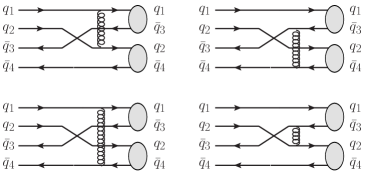
By using the spectrum obtained from NRPQM, we further evaluate the fall-apart decays of the $T_{(4Q)}$ states in a quark-exchange model Barnes:2000hu . The interactions $V_{ij}$ between inner quarks of final hadrons $B$ and $C$ may be the sources of the fall-apart decays of a $T_{(4Q)}$ state via the quark rearrangement. The decay amplitude $\mathcal{M}(A\to BC)$ of $T_{(4Q)}$ state is described by:

$$\mathcal{M}(A\to BC)=-\sqrt{(2\pi)^{3}}\sqrt{8M_{A}E_{B}E_{C}}\left\langle BC|\underset{i<j}{\sum}V_{ij}|A\right\rangle,$$

(6)

where $A$ stands for the initial tetraquark state, $BC$ stands for the final hadron pair. $M_{A}$ is the mass of the initial state, and $E_{B}$ and $E_{C}$ are the energies of the final states $B$ and $C$, respectively. The decay width $\Gamma$ of $A\to BC$ can be described by:

$\displaystyle\Gamma$

$\displaystyle=$

$\displaystyle\frac{1}{2J_{A}+1}\frac{|\boldsymbol{p}|}{8\pi M_{A}^{2}}\left|\mathcal{M}(A\to BC)\right|^{2},$

(7)

where $|\boldsymbol{p}|$ is magnitude of the momentum for the final states $B$ and $C$. The potentials $V_{ij}$ ($ij\neq 13,24$ or $ij\neq 14,23$) between inner quarks of final hadrons $B$ and $C$, as shown in Fig. 3, are taken the same as our mass calculations. The calculation of the decay amplitude for a $T_{(4Q)}$ state is indeed a tedious task, some details are given in the appendix. This model has been developed and applied to the study of the hidden-charm decay properties for the multiquark states in the literature Wang:2019spc ; Xiao:2019spy ; Wang:2020prk ; Han:2022fup ; Liu:2022hbk , and a lot of inspiring results are obtained. For simplicity, the wave functions of the $A,B,C$ hadron states are parametrized out in a single harmonic oscillator form by fitting the wave functions calculated from our potential model Liu:2019vtx ; Liu:2020lpw ; Liu:2021rtn . The harmonic oscillator parameters for the final meson states and initial tetraquark states are collected in Tables 4 and  5 of the appendix, respectively.

References

- (1) M. Gell-Mann, A Schematic Model of Baryons and Mesons, Phys. Lett. 8, 214 (1964).
- (2) G. Zweig, An SU(3) model for strong interaction symmetry and its breaking. Version 1, CERN-TH-401.
- (3) S. K. Choi et al. [Belle Collaboration], Observation of a narrow charmonium - like state in exclusive decays, Phys. Rev. Lett. 91, 262001 (2003).
- (4) S. L. Olsen, T. Skwarnicki, and D. Zieminska, Nonstandard heavy mesons and baryons: Experimental evidence, Rev. Mod. Phys. 90, 015003 (2018).
- (5) R. F. Lebed, R. E. Mitchell, and E. S. Swanson, Heavy-Quark QCD exotica, Prog. Part. Nucl. Phys. 93, 143 (2017).
- (6) H. X. Chen, W. Chen, X. Liu and S. L. Zhu, The hidden-charm pentaquark and tetraquark states, Phys. Rep. 639, 1 (2016).
- (7) A. Ali, J. S. Lange and S. Stone, Exotics: Heavy pentaquarks and tetraquarks, Prog. Part. Nucl. Phys. 97, 123 (2017).
- (8) A. Esposito, A. Pilloni, and A. D. Polosa, Multiquark resonances, Phys. Rep. 668, 1 (2016).
- (9) Y. R. Liu, H. X. Chen, W. Chen, X. Liu and S. L. Zhu, Pentaquark and Tetraquark states, Prog. Part. Nucl. Phys. 107, 237 (2019).
- (10) F. K. Guo, C. Hanhart, U. G. Meissner, Q. Wang, Q. Zhao and B. S. Zou, Hadronic molecules, Rev. Mod. Phys. 90, 015004 (2018).
- (11) J. P. Ader, J. M. Richard and P. Taxil, Do narrow heavy multi - quark states exist, Phys. Rev. D 25, 2370 (1982).
- (12) Y. Iwasaki, A possible model for new resonances-exotics and hidden charm, Prog. Theor. Phys. 54, 492 (1975).
- (13) S. Zouzou, B. Silvestre-Brac, C. Gignoux and J. M. Richard, Four quark bound states, Z. Phys. C 30, 457 (1986).
- (14) L. Heller and J. A. Tjon, On bound states of heavy systems, Phys. Rev. D 32, 755 (1985).
- (15) R. J. Lloyd and J. P. Vary, All charm tetraquarks, Phys. Rev. D 70, 014009 (2004).
- (16) N. Barnea, J. Vijande, and A. Valcarce, Four-quark spectroscopy within the hyperspherical formalism, Phys. Rev. D 73, 054004 (2006).
- (17) J. Vijande, A. Valcarce, and N. Barnea, Exotic meson-meson molecules and compact four-quark states, Phys. Rev. D 79, 074010 (2009).
- (18) M. N. Anwar, J. Ferretti, F. K. Guo, E. Santopinto, and B. S. Zou, Spectroscopy and decays of the fully-heavy tetraquarks, Eur. Phys. J. C 78, 647 (2018).
- (19) M. Karliner, S. Nussinov, and J. L. Rosner, states: Masses, production, and decays, Phys. Rev. D 95, 034011 (2017).
- (20) Y. Bai, S. Lu, and J. Osborne, Beauty-full tetraquarks, Phys. Lett. B 798, 134930 (2019).
- (21) A. V. Berezhnoy, A. V. Luchinsky and A. A. Novoselov, Tetraquarks composed of 4 heavy quarks, Phys. Rev. D 86, 034004 (2012).
- (22) Z. G. Wang, Analysis of the tetraquark states with QCD sum rules, Eur. Phys. J. C 77, 432 (2017).
- (23) Z. G. Wang and Z. Y. Di, Analysis of the vector and axialvector tetraquark states with QCD sum rules, Acta Phys. Polon. B 50, 1335 (2019).
- (24) V. R. Debastiani and F. S. Navarra, A non-relativistic model for the tetraquark, Chin.Phys.C 43,013105(2018).
- (25) A. Esposito and A. D. Polosa, A di-bottomonium at the LHC, Eur Phys J.C 78.782(2018).
- (26) P. Lundhammar and T. Ohlsson, Nonrelativistic model of tetraquarks and predictions for their masses from fits to charmed and bottom meson data, Phys. Rev. D 102, 054018 (2020).
- (27) J. M. Richard, A. Valcarce, and J. Vijande, Few-body quark dynamics for doubly heavy baryons and tetraquarks, Phys. Rev. C 97, 035211 (2018).
- (28) J. M. Richard, A. Valcarce, and J. Vijande, String dynamics and metastability of all-heavy tetraquarks, Phys. Rev. D 95, 054019 (2017).
- (29) J. Wu, Y. R. Liu, K. Chen, X. Liu, and S. L. Zhu, Heavy-flavored tetraquark states with the configuration, Phys. Rev. D 97, 094015 (2018).
- (30) C. Hughes, E. Eichten, and C. T. H. Davies, Searching for beauty-fully bound tetraquarks using lattice nonrelativistic QCD, Phys. Rev. D 97, 054505 (2018).
- (31) W. Chen, H. X. Chen, X. Liu, T. G. Steele and S. L. Zhu, Hunting for exotic doubly hidden-charm/bottom tetraquark states, Phys. Lett. B 773, 247 (2017).
- (32) W. Chen, H. X. Chen, X. Liu, T. G. Steele and S. L. Zhu, Doubly hidden-charm/bottom tetraquark states, EPJ Web Conf. 182, 02028 (2018).
- (33) M. S. Liu, Q. F. Lü, X. H. Zhong and Q. Zhao, All-heavy tetraquarks, Phys. Rev. D 100, 016006 (2019).
- (34) C. Deng, H. Chen and J. Ping, Towards the understanding of fully-heavy tetraquark states from various models, Phys. Rev. D 103, 014001 (2021).
- (35) G. J. Wang, L. Meng and S. L. Zhu, Spectrum of the fully-heavy tetraquark state , Phys. Rev. D 100, 096013 (2019).
- (36) M. A. Bedolla, J. Ferretti, C. D. Roberts and E. Santopinto, Spectrum of fully-heavy tetraquarks from a diquark+antidiquark perspective, Eur. Phys. J. C 80, 1004 (2020).
- (37) X. Chen, Fully-charm tetraquarks: , arXiv:2001.06755 [hep-ph].
- (38) R. Aaij et al. [LHCb], Observation of structure in the -pair mass spectrum, Sci. Bull. 65, no.23, 1983-1993 (2020).
- (39) G. Aad et al. [ATLAS], Observation of an Excess of Dicharmonium Events in the Four-Muon Final State with the ATLAS Detector, Phys. Rev. Lett. 131, 151902 (2023).
- (40) A. Hayrapetyan et al. [CMS], Observation of new structure in the J/J/ mass spectrum in proton-proton collisions at = 13 TeV, [arXiv:2306.07164 [hep-ex]].
- (41) W. C. Dong and Z. G. Wang, Going in quest of potential tetraquark interpretations for the newly observed states in light of the diquark-antidiquark scenarios, Phys. Rev. D 107, no.7, 074010 (2023)
- (42) W. Chen, Q. N. Wang, Z. Y. Yang, H. X. Chen, X. Liu, T. G. Steele and S. L. Zhu, Searching for fully-heavy tetraquark states in QCD moment sum rules, Nucl. Part. Phys. Proc. 318-323, 73-77 (2022).
- (43) R. N. Faustov, V. O. Galkin and E. M. Savchenko, Fully-heavy tetraquark spectroscopy in the relativistic quark model, Symmetry 14, 2504 (2022)
- (44) P. Y. Niu, E. Wang, Q. Wang and S. Yang, Determine the quantum numbers of from photon-photon fusion in ultra-peripheral heavy ion collisions, [arXiv:2209.01924 [hep-ph]].
- (45) G. J. Wang, Q. Meng and M. Oka, S-wave fully charmed tetraquark resonant states, Phys. Rev. D 106, 096005 (2022).
- (46) H. T. An, S. Q. Luo, Z. W. Liu and X. Liu, Systematic search of fully heavy tetraquark states, Eur. Phys. J. C 83, 740 (2023).
- (47) V. Biloshytskyi, V. Pascalutsa, L. Harland-Lang, B. Malaescu, K. Schmieden and M. Schott, Two-photon decay of X(6900) from light-by-light scattering at the LHC, Phys. Rev. D 106, L111902 (2022).
- (48) J. Z. Wang and X. Liu, Improved understanding of the peaking phenomenon existing in the new di-J/ invariant mass spectrum from the CMS Collaboration, Phys. Rev. D 106, no.5, 054015 (2022).
- (49) C. Gong, M. C. Du and Q. Zhao, Pseudoscalar charmonium pair interactions via the Pomeron exchange mechanism, Phys. Rev. D 106, no.5, 054011 (2022).
- (50) R. H. Wu, Y. S. Zuo, C. Y. Wang, C. Meng, Y. Q. Ma and K. T. Chao, NLO results with operator mixing for fully heavy tetraquarks in QCD sum rules, JHEP 11, 023 (2022).
- (51) Z. Zhuang, Y. Zhang, Y. Ma and Q. Wang, Lineshape of the compact fully heavy tetraquark, Phys. Rev. D 105, 054026 (2022).
- (52) Y. Yan, Y. Wu, X. Hu, H. Huang and J. Ping, Fully heavy pentaquarks in quark models, Phys. Rev. D 105, 014027 (2022).
- (53) Q. N. Wang, Z. Y. Yang and W. Chen, Exotic fully-heavy tetraquark states in color configuration, Phys. Rev. D 104, 114037 (2021).
- (54) A. J. Majarshin, Y. A. Luo, F. Pan and J. Segovia, Bosonic algebraic approach applied to the tetraquarks, Phys. Rev. D 105, 054024 (2022).
- (55) Z. Zhao, K. Xu, A. Kaewsnod, X. Liu, A. Limphirat and Y. Yan, Study of charmoniumlike and fully-charm tetraquark spectroscopy, Phys. Rev. D 103, 116027 (2021).
- (56) Q. Li, C. H. Chang, G. L. Wang and T. Wang, Mass spectra and wave functions of tetraquarks, Phys. Rev. D 104, 014018 (2021).
- (57) G. J. Wang, L. Meng, M. Oka and S. L. Zhu, Higher fully charmed tetraquarks: Radial excitations and P-wave states, Phys. Rev. D 104, 036016 (2021).
- (58) G. Yang, J. Ping and J. Segovia, Exotic resonances of fully-heavy tetraquarks in a lattice-QCD insipired quark model, Phys. Rev. D 104, 014006 (2021).
- (59) Y. Huang, F. Feng, Y. Jia, W. L. Sang, D. S. Yang and J. Y. Zhang, Inclusive production of fully-charmed tetraquark at B factory, Chin. Phys. C 45, 093101 (2021).
- (60) V. P. Gonçalves and B. D. Moreira, Fully - heavy tetraquark production by interactions in hadronic collisions at the LHC, Phys. Lett. B 816, 136249 (2021).
- (61) M. Z. Liu and L. S. Geng, Is the heavy anti-quark diquark symmetry partner of ?, Eur. Phys. J. C 81, 179 (2021).
- (62) J. Z. Wang, X. Liu and T. Matsuki, Fully-heavy structures in the invariant mass spectrum of , , , and at hadron colliders, Phys. Lett. B 816, 136209 (2021).
- (63) B. D. Wan and C. F. Qiao, Gluonic tetracharm configuration of , Phys. Lett. B 817, 136339 (2021).
- (64) C. Gong, M. C. Du, Q. Zhao, X. H. Zhong and B. Zhou, Nature of X(6900) and its production mechanism at LHCb, Phys. Lett. B 824, 136794 (2022).
- (65) Q. F. Cao, H. Chen, H. R. Qi and H. Q. Zheng, Some remarks on X(6900), Chin. Phys. C 45, 103102 (2021).
- (66) Z. H. Guo and J. A. Oller, Insights into the inner structures of the fully charmed tetraquark state , Phys. Rev. D 103, 034024 (2021).
- (67) R. Zhu, Fully-heavy tetraquark spectra and production at hadron colliders, Nucl. Phys. B 966, 115393 (2021).
- (68) J. R. Zhang, fully-charmed tetraquark states, Phys. Rev. D 103, 014018 (2021).
- (69) F. Feng, Y. Huang, Y. Jia, W. L. Sang, X. Xiong and J. Y. Zhang, Fragmentation production of fully-charmed tetraquarks at the LHC, Phys. Rev. D 106, 114029 (2022).
- (70) Y. Q. Ma and H. F. Zhang, Exploring the Di- Resonances around 6.9 Based on Perturbative QCD, [arXiv:2009.08376 [hep-ph]].
- (71) X. K. Dong, V. Baru, F. K. Guo, C. Hanhart and A. Nefediev, Coupled-Channel Interpretation of the LHCb Double- Spectrum and Hints of a New State Near the Threshold, Phys. Rev. Lett. 126, no.13, 132001 (2021) [erratum: Phys. Rev. Lett. 127, 119901 (2021)].
- (72) Z. G. Wang, Revisit the tetraquark candidates in the mass spectrum, Int. J. Mod. Phys. A 36, 2150014 (2021).
- (73) M. Karliner and J. L. Rosner, Interpretation of structure in the di- spectrum, Phys. Rev. D 102, 114039 (2020).
- (74) J. Z. Wang, D. Y. Chen, X. Liu and T. Matsuki, Producing fully charm structures in the -pair invariant mass spectrum, Phys. Rev. D 103, 071503 (2021).
- (75) J. F. Giron and R. F. Lebed, Simple spectrum of states in the dynamical diquark model, Phys. Rev. D 102, 074003 (2020).
- (76) X. Y. Wang, Q. Y. Lin, H. Xu, Y. P. Xie, Y. Huang and X. Chen, Discovery potential for the LHCb fully-charm tetraquark state via annihilation reaction, Phys. Rev. D 102, 116014 (2020).
- (77) H. X. Chen, W. Chen, X. Liu and S. L. Zhu, Strong decays of fully-charm tetraquarks into di-charmonia, Sci. Bull. 65, 1994-2000 (2020).
- (78) H. X. Chen, Y. X. Yan and W. Chen, Decay behaviors of the fully bottom and fully charm tetraquark states, Phys. Rev. D 106, 094019 (2022).
- (79) C. Becchi, J. Ferretti, A. Giachino, L. Maiani and E. Santopinto, A study of tetraquark decays in 4 muons and in at LHC, Phys. Lett. B 811, 135952 (2020).
- (80) C. Becchi, A. Giachino, L. Maiani and E. Santopinto, Search for tetraquark decays in 4 muons, , and channels at LHC, Phys. Lett. B 806, 135495 (2020).
- (81) Z. G. Wang, Tetraquark candidates in the LHCb’s di- mass spectrum, Chin. Phys. C 44, 113106 (2020).
- (82) G. Yang, J. Ping, L. He and Q. Wang, Potential model prediction of fully-heavy tetraquarks (), [arXiv:2006.13756 [hep-ph]].
- (83) P. Niu, Z. Zhang, Q. Wang and M. L. Du, The third peak structure in the double spectrum, Sci. Bull. 68, 800-803 (2023).
- (84) Z. R. Liang and D. L. Yao, On the nature of and other structures in the LHCb di- spectrum, Rev. Mex. Fis. Suppl. 3, no.3, 0308042 (2022).
- (85) Z. R. Liang, X. Y. Wu and D. L. Yao, Hunting for states in the recent LHCb di- invariant mass spectrum, Phys. Rev. D 104, 034034 (2021).
- (86) X. K. Dong, V. Baru, F. K. Guo, C. Hanhart, A. Nefediev and B. S. Zou, Is the existence of a J/J/ bound state plausible?, Sci. Bull. 66, 2462-2470 (2021).
- (87) H. W. Ke, X. Han, X. H. Liu and Y. L. Shi, Tetraquark state and the interaction between diquark and antidiquark, Eur. Phys. J. C 81, 427 (2021).
- (88) B. C. Yang, L. Tang and C. F. Qiao, Scalar fully-heavy tetraquark states in QCD sum rules, Eur. Phys. J. C 81, 324 (2021).
- (89) X. Z. Weng, X. L. Chen, W. Z. Deng and S. L. Zhu, Systematics of fully heavy tetraquarks, Phys. Rev. D 103, 034001 (2021).
- (90) J. Zhao, S. Shi and P. Zhuang, Fully-heavy tetraquarks in a strongly interacting medium, Phys. Rev. D 102, 114001 (2020).
- (91) S. Q. Kuang, Q. Zhou, D. Guo, Q. H. Yang and L. Y. Dai, Study of with unitarized coupled channel scattering amplitudes, Eur. Phys. J. C 83, 383 (2023).
- (92) Q. Zhou, D. Guo, S. Q. Kuang, Q. H. Yang and L. Y. Dai, Nature of the X(6900) in partial wave decomposition of scattering, Phys. Rev. D 106, L111502 (2022).
- (93) F. X. Liu, M. S. Liu, X. H. Zhong and Q. Zhao, Higher mass spectra of the fully-charmed and fully-bottom tetraquarks, Phys. Rev. D 104, 116029 (2021).
- (94) E. Eichten, K. Gottfried, T. Kinoshita, K. D. Lane and T. M. Yan, Charmonium: The Model, Phys. Rev. D 17, 3090 (1978) Erratum: [Phys. Rev. D 21, 313 (1980)].
- (95) Q. F. Lü, D. Y. Chen and Y. B. Dong, Masses of fully heavy tetraquarks in an extended relativized quark model, Eur. Phys. J. C 80, 871 (2020).
- (96) W. J. Deng, H. Liu, L. C. Gui and X. H. Zhong, Charmonium spectrum and their electromagnetic transitions with higher multipole contributions, Phys. Rev. D 95, 034026 (2017).
- (97) M. S. Liu, Q. F. Lü and X. H. Zhong, Triply charmed and bottom baryons in a constituent quark model, Phys. Rev. D 101, 074031 (2020).
- (98) T. Barnes, N. Black and E. S. Swanson, Meson meson scattering in the quark model: Spin dependence and exotic channels, Phys. Rev. C 63, 025204 (2001).
- (99) G. J. Wang, L. Y. Xiao, R. Chen, X. H. Liu, X. Liu and S. L. Zhu, Probing hidden-charm decay properties of states in a molecular scenario, Phys. Rev. D 102, 036012 (2020).
- (100) L. Y. Xiao, G. J. Wang and S. L. Zhu, Hidden-charm strong decays of the states, Phys. Rev. D 101, 054001 (2020).
- (101) G. J. Wang, L. Meng, L. Y. Xiao, M. Oka and S. L. Zhu, Mass spectrum and strong decays of tetraquark states, Eur. Phys. J. C 81, 188 (2021).
- (102) S. Han and L. Y. Xiao, Aspects of and , Phys. Rev. D 105, 054008 (2022).
- (103) F. X. Liu, R. H. Ni, X. H. Zhong and Q. Zhao, Charmed-strange tetraquarks and their decays in a potential quark model, Phys. Rev. D 107, 096020 (2023).
- (104) F. X. Liu, M. S. Liu, X. H. Zhong and Q. Zhao, Fully-strange tetraquark spectrum and possible experimental evidence, Phys. Rev. D 103, 016016 (2021).
- (105) D. M. Brink and F. Stancu, etraquarks with heavy flavors, Phys. Rev. D 57, 6778 (1998).
- (106) D. V. Fedorov, Analytic matrix elements with shifted correlated Gaussians, Few Body Syst. 58, 21 (2017).
Appendix A
The calculation of the decay amplitude of a state is indeed a tedious task. For simplicity, the spatial wave functions for the hadron states are adopted a harmonic oscillator form, the harmonic oscillator parameters are determined by fitting the wave functions calculated from the potential model. These parameters have been given in Tab. 4 and Tab. 5.
. State Mass Mass 2984 658 9378 1160 3097 564 9436 1096 (2S) 3635 506 (2S) 9973 858 (2S) 3679 470 (2S) 9989 822 3417 533 9845 822 3522 459 9899 731 3516 459 9891 759 3552 429 9914 705
Taking as an example, from Tab. 1 one can obtain the wave function for the initial state, i.e.,