Full-State Prescribed Performance-Based Consensus of Double-Integrator Multi-Agent Systems with Jointly Connected Topologies
Abstract
This paper addresses the full-state prescribed performance-based consensus problem for double-integrator multi-agent systems with jointly connected topologies. To improve the transient performance, a distributed prescribed performance control protocol consisting of the transformed relative position and the transformed relative velocity is proposed, where the communication topology satisfies the jointly connected assumption. Different from the existing literatures, two independent transient performance specifications imposed on relative positions and relative velocities can be guaranteed simultaneously. A numerical example is ultimately used to validate the effectiveness of proposed protocol.
Index Terms:
Consensus, prescribed performance control, jointly connected topologies, double-integrator dynamics, multi-agent systems.I Introduction
Recently, multi-agent systems (MASs) have received considerable attention in completing a range of tasks such as rescue, transportation, and exploration, mainly because they are efficient and inexpensive[1]. More and more research topics were conducted on the cooperative control of MASs, in which consensus reaching is a classical topic[2]. The consensus of MASs was achieved for different dynamics, including single-integrator dynamic [3], double-integrator dynamic [4, 5], linear dynamic [6, 7], and nonlinear dynamic [8].
Although the control protocols in literatures [3, 4, 5, 6, 7, 8] achieved asymptotic convergence as expected, the steady and transient-state performance during the convergence process were usually neglected. To address this issue, the prescribed performance control (PPC) method based on performance functions and error transformation functions was first proposed in [9], where the tracking errors were confined within an arbitrarily small residual set, with predefined minimum convergence rate and maximum overshoot. Soon afterwards, the PPC method was applied to the single-integrator and double-integrator MASs to achieve consensus [10, 11], in which the trajectories of relative positions defined as the difference among the connected agents respected the performance bound.
In detail, we then review the application of PPC method in MASs. In [11], Macellari et al. proposed a distributed control protocol consisting of a linear combination term between relative positions and relative velocities as well as an additional absolute velocity term, such that the performance specifications imposed on the above linear combination term can be guaranteed. The performance specifications are imposed on the linear combination term, however, relative positions and relative velocities cannot be confined within their respective performance bounds. In terms of the controller designed in [11], modulating the performance specifications on relative velocities makes the stability analysis more complicated. In [12], the designed controller guaranteed a transient performance for the robot joint position and velocity tracking errors. Recently, more research results on this topic can be found in [13, 14, 15, 16].
Up to this point, no research results were found in which the relative positions and relative velocities among connected agents evolve within their respective predefined performance bounds. In short, these independent performance specifications associated with positions and velocities form the so-called full-state prescribed performance for double-integrator MASs. The above literatures mainly considered fixed topology, while switching topology cases caused by the failures and changes of communication link among neighboring agents are rarely involved [17, 18].
Motivated by the above discussion, the full-state prescribed performance-based consensus control problem for double-integrator MASs with jointly connected topologies is addressed. To be specific, a vital advantage of this paper, is that a novel distributed control protocol is designed to improve the transient performance of both relative positions and relative velocities, which are different from the existing PPC methods based on MASs with single-integrator [10, 13] and double-integrator [11, 15, 16] dynamics. Furthermore, considering the jointly connected topology case, all agents are driven to converge asymptotically by applying prescribed performance-based control protocol, and the design parameters are independent of topology information. It is worth mentioning that topology graphs are no longer limited to tree and connected graph cases [13, 14, 15], and MASs can achieve the accurate consensus rather than practical consensus [12, 14].
II Background and Problem Formulation
II-A Notations and Graph Theory
For convenience, we summarize some notations as follows. : the set of dimension real column vectors; : the identity matrix; : the transposition of ; : diagonal matrix with entries .
An undirected graph is composed of the node set and edge set , where , is a piecewise constant switching signal. Let be the adjacency matrix where if and otherwise. The neighbor set of node is . The Laplacian matrix is defined as , where degree matrix with diagonal entry . The incidence matrix is defined as , , where is a edge set. Besides, edge , is described as edge . For the connected graph, the edge Laplacian matrix is positive semidefinite [15, 16].
Suppose there exists an infinite, bounded and contiguous time interval , where and for positive constant . During each interval , there is a sequence of nonoverlapping subintervals , with and , satisfying , , and is called dwell time. The graph is fixed for . If the union graph is connected, then is jointly connected.
II-B Prescribed Performance Control
Partly referring to [9, 10], the prescribed performance is achieved if element of tracking errors evolves within the following performance bounds
| (1) |
where performance function with positive constants , and . Next, we normalize by , and define the prescribed performance regions with . Let and . Thus , is equivalent to (1).
The normalized value is transformed by tracking error transformation functions that define a smooth and strictly increasing mapping , with . More specifically, one can select transformation function as
| (2) |
The time derivative of is
| (3) |
with and . Let . By calculating, the following inequality
| (4) |
holds for a positive constant . In view of the properties of transformation function , with constants , the following inequality
| (5) |
holds[12], where , , , and .
Lemma 1 ([19])
Given any positive constants and , we have
for all , with constant .
II-C Problem Formulation
Consider a MAS with agents modeled by double-integrator dynamic
| (6) |
where represent the position, velocity and control input of agent , respectively.
Assumption 1
The graph are jointly connected across each interval , .
Based on the matrix , we define relative position
and relative velocity
where edge is connected between agents and . Letting , , and , we have and .
In the following, the performance specifications are imposed on tracking errors and . For convenience, the symbol of section II-B is replaced with and respectively.
Objective: For the MAS (6) with switching topologies and performance functions and , design a distributed control protocol to achieve consensus in the sense of
while transient performance and , are guaranteed.
III Main Results
To achieve the above objective, we propose the prescribed performance control protocol as follows
| (7) |
where is a positive constant. Invoking (6) and (III), the closed-loop system is rewritten as
| (8) |
Remark 1
Compared to existing literatures [10, 13, 20] based on single-integrator MASs, the velocity information of double-integrator MAS (6) makes controller design and stability analysis more complicated. The control protocol (III) consists of two nonlinear error transformation terms, which is a vital advantage in improving the transient performance of relative positions and relative velocities, instead of single relative positions mentioned in [11].
Partly inspired by [16], the following lemmas are obtained.
Proof:
Simplifying the equality (III), we obtain
| (10) |
where , for . By solving differential equation (10), one has, with ,
Since and , and and are bounded, and , are continuous and bounded. By calculating, is bounded, and thus and , are continuous and bounded. In return, the same conclusion can be reached for and , . Letting , it follows from [19] that and , are uniformly continuous and bounded. The proof is completed. ∎
Theorem 1
Proof:
The proof is divided into four steps. To begin with, there exists a unique maximum solution over the set , i.e., , . Nextly, it is verified that the protocol ensures, and for are bounded and strictly within the compact subset of and respectively. Then proof by contradiction leads to . The consensus is finally proven by Barbalat’s Lemma.
Phase I. Since and , one has . By calculating the derivative of and , it is confirmed that is continuous and locally Lipschitz on . In view of Theorem 54 of [22], there exists the maximal solution , and hence is guaranteed for .
Phase II. It follows from Phase I that and , satisfy bound (1) respectively. Consider a potential function as follows
| (11) |
where , , , and . Computing , we obtain
By the Young’s inequality [14], with positive constants and , one has
Combining the above inequalities and inequality (4) gives
By feat of Lemma 3, and are bounded and the upper bound are supposed as and respectively. On account of the boundedness of for , is bounded and its upper bound is recorded as . With , one has
where , , , , and . By Lemma 1, the following holds
for all and . By applying the inequality (5), we have
| (12) |
It can be seen that is guaranteed by
within . By using the inverse operation of the transformation function , we obtain, with ,
Phase III. Up to this point, we prove that can be extended to . It is obtained from (III) that
where and . is obviously a nonempty subset of . Suppose , it is inferred from Proposition C.3.6 of [22] that the inequality holds for a instant , which is a clear contradiction. From Theorem of [19], one obtain and , thus is finite and bounded, .
Phase IV. We finally prove that and converge to zero as . Taking a part of calculation in (III) gives
| (13) |
where . Since and , is bounded and exists. Given an infinite sequences , , by utilizing Cauchy’s Convergence Criterion, one has, for , , such that ,
| (14) |
It follows that
| (15) |
For each subinterval , , one has
Combining the above two inequalities gives
Since finite switches take place during , the number is finite for . It implies that, with a bounded constant ,
Since and are bounded, and are bounded, . Utilizing the Barbalat’s Lemma [16] gives and , and consequently, and . The proof is completed. ∎
Remark 2
Generally speaking, the controller is updated based on the connected agents’ state feedback. As the graph switches, the neighbor set of agent will change. By applying the control protocol (III), the consensus control problem caused by switching topologies is solved. If the graph is a tree, the edge Laplacian matrix is positive definite. However, this positive definiteness condition is not required in the proof, such that protocol (III) is applicable to generally connected graphs containing cycles.
Remark 3
IV Simulation
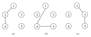
Consider a MAS composed of agents with the dynamic model (6) and (III). Suppose the topology graph described in Fig.1 switches as , with the dwelling time s. We choose performance functions and for all edges. Then we have and , and hence and . For all edges, the same transformation functions are selected as
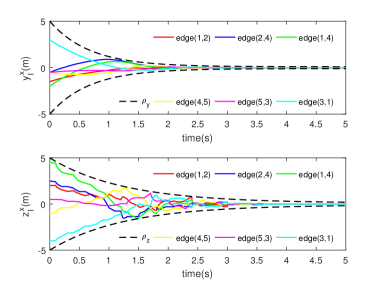
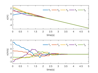
The initial positions of agents are , and initial velocities are . For Theorem 1, we choose and . The state trajectories of all agents for from to s, are depicted in Figs. 3 and 3. It follows from Fig. 3 that the relative positions and relative velocities are confined within the performance bounds as expected, and the state consensus of all agents is eventually achieved as shown in Fig. 3.
V Conclusion
This paper addresses the full-state prescribed performance-based consensus problem for double-integrator MASs with jointly connected topologies. A distributed prescribed performance control protocol is proposed such that the relative positions and relative velocities are constrained within the respective performance bounds. The proposed protocol drives all agents to achieve consensus with jointly connected topologies. Future research topics focus on more general agent dynamics.
References
- [1] X. M. Zhang, Q. L. Han, X. Ge, D. Ding, L. Ding, D. Yue, and C. Peng, “Networked control systems:a survey of trends and techniques,” IEEE/CAA Journal of Automatica Sinica, vol. 007, no. 001, pp. 1–17, 2020.
- [2] J. Qin, Q. Ma, Y. Shi, and L. Wang, “Recent advances in consensus of multi-agent systems: A brief survey,” IEEE Transactions on Industrial Electronics, vol. 64, no. 6, pp. 4972–4983, 2017.
- [3] R. Olfati-Saber and R. M. Murray, “Consensus problems in networks of agents with switching topology and time-delays,” IEEE Transactions on Automatic Control, vol. 49, no. 9, pp. 1520–1533, 2004.
- [4] W. Yu, L. Zhou, X. Yu, J. Lü, and R. Lu, “Consensus in multi-agent systems with second-order dynamics and sampled data,” IEEE Transactions on Industrial Informatics, vol. 9, no. 4, pp. 2137–2146, 2013.
- [5] J. Zeng, P. Wang, H. Su, and C. Xu, “Second-order consensus for multi-agent systems with various intelligent levels via intermittent sampled-data control,” IEEE Transactions on Circuits and Systems II: Express Briefs, vol. 69, no. 12, pp. 4899–4903, 2022.
- [6] Y. Ren, Q. Wang, and Z. Duan, “Optimal distributed leader-following consensus of linear multi-agent systems: A dynamic average consensus-based approach,” IEEE Transactions on Circuits and Systems II: Express Briefs, vol. 69, no. 3, pp. 1208–1212, 2021.
- [7] Y. Sun and S. Peng, “Consensus of discrete-time leader-following linear multi-agent systems under lyapunov-function-based event-triggered mechanism,” IEEE Transactions on Circuits and Systems II: Express Briefs, vol. 70, no. 12, pp. 4409 – 4413, 2023.
- [8] X. Tan, M. Cao, and J. Cao, “Distributed dynamic event-based control for nonlinear multi-agent systems,” IEEE Transactions on Circuits and Systems II: Express Briefs, vol. 68, no. 2, pp. 687–691, 2020.
- [9] C. P. Bechlioulis and G. A. Rovithakis, “Robust adaptive control of feedback linearizable MIMO nonlinear systems with prescribed performance,” IEEE Transactions on Automatic Control, vol. 53, no. 9, pp. 2090–2099, 2008.
- [10] Y. Karayiannidis, D. V. Dimarogonas, and D. Kragic, “Multi-agent average consensus control with prescribed performance guarantees,” in IEEE Conference on Decision & Control, 2012, pp. 2219–2225.
- [11] L. Macellari, Y. Karayiannidis, and D. V. Dimarogonas, “Multi-agent second order average consensus with prescribed transient behavior,” IEEE Transactions on Automatic Control, vol. 62, no. 10, pp. 5282–5288, 2017.
- [12] Y. Karayiannidis, D. Papageorgiou, and Z. Doulgeri, “A model-free controller for guaranteed prescribed performance tracking of both robot joint positions and velocities,” IEEE Robotics & Automation Letters, vol. 1, no. 1, pp. 267–273, 2016.
- [13] F. Chen and D. V. Dimarogonas, “Consensus control for leader-follower multi-agent systems under prescribed performance guarantees,” in 2019 IEEE 58th Conference on Decision and Control. IEEE, 2019, pp. 4785–4790.
- [14] ——, “Second order consensus for leader-follower multi-agent systems with prescribed performance,” in IFAC-PapersOnLine, vol. 52, no. 20, 2019, pp. 103–108.
- [15] Y. Hou and W. Hu, “Event-triggered consensus of second-order multi-agent systems with prescribed performance,” in 2021 China Automation Congress (CAC), 2021, pp. 1146–1150.
- [16] Y. Hou and B. Cheng, “Event-based consensus of double-integrator multi-agent systems: A prescribed performance control approach,” IEEE Transactions on Circuits and Systems II: Express Briefs, early access, November. 15, 2023, doi: 10.1109/TCSII.2023.3332746.
- [17] B. Cheng, X. Wang, and Z. Li, “Event-triggered consensus of homogeneous and heterogeneous multiagent systems with jointly connected switching topologies,” IEEE Transactions on Cybernetics, vol. 49, no. 12, pp. 4421–4430, 2018.
- [18] X. Wan, Y. Guo, and X. Wu, “Differentially private consensus for multi-agent systems under switching topology,” IEEE Transactions on Circuits and Systems II: Express Briefs, vol. 70, no. 9, pp. 3499–3503, 2023.
- [19] C. J. Stamouli, C. P. Bechlioulis, and K. J. Kyriakopoulos, “Robust dynamic average consensus with prescribed transient and steady state performance,” Automatica, vol. 144, p. 110503, 2022.
- [20] E. Restrepo and D. V. Dimarogonas, “On asymptotic stability of leader–follower multiagent systems under transient constraints,” IEEE Control Systems Letters, vol. 6, pp. 3164–3169, 2022.
- [21] Y. Hou, W. Hu, J. Li, and T. Huang, “Prescribed performance control for double-integrator multi-agent systems: A unified event-triggered consensus framework,” IEEE Transactions on Circuits and Systems I: Regular Papers, 2023, under review.
- [22] E. D. Sontag, Mathematical control theory. London, U. K.: Springer, 1998.