Full-Duplex ISAC-Enabled D2D Underlaid Cellular Networks: Joint Transceiver Beamforming and Power Allocation

WITH the explosive growth of the Internet of Things (IoT) devices, spectrum resource congestion is becoming increasingly prominent. Besides, many emerging applications in the sixth generation (6G), such as intelligent transportation and human-computer interaction, demand both high-quality communications and high-precision sensing simultaneously. These practical needs motivate the design of integrated sensing and communication (ISAC) systems, which has attracted extensive attention from both industry and academia [1]. Moreover, advancements in technologies such as multiple-input multiple-output (MIMO) [2], signal processing technologies for ISAC [3] and hardware design enable sensing and communication functionalities to be implemented using the same hardware and share same spectrum resource to achieve reliable communications and sensing, which could effectively improve spectral efficiency and energy efficiency.

In a MIMO ISAC system, beamforming plays a key role, where the spatial degrees of freedom (DoFs) provided by MIMO can be exploited to achieve substantial gains in both sensing and communications. Many existing works focus on the design of transmit beamforming [4, 5, 6, 7, 8, 9, 10], with optimization problems centered around two key metrics for sensing: 1) Beampattern gains at the direction of targets; 2) Beampattern template matching. Under the first metric, He et al in [4] optimized the transmit beampattern by formulating an energy efficiency maximization problem while ensuring the beampattern gains of targets and the SINR requirements of communication users. The transmit beampattern design was also considered in NOMA-ISAC systems [5], RIS-aided ISAC systems [6], and secure ISAC systems [7]. In [5], a weighted objective function, which involves the beampattern gain at a target and the SINR at communication users, is maximized. In [6], a reconfigurable intelligent surface (RIS) is employed to enhance the beampattern gain at the target direction by establishing an extra reflective link. In a secure ISAC system in [7], the beampattern gain at the target (eavesdropper) is maximized while guaranteeing the secret rate and communication rate of legitimate users. Under the second metric, in [8], the matching error between the designed and desired beampattern is minimized, incorporating the outage probability and power consumption constraints. Based on [8], in [9] and [10], the authors considered a weighted minimization problem of matching error and cross-correlation among beampatterns of multiple targets. However, these works focus on transmit beampatterns and ignore the reception of radar echo, which fails to capture the property of the receive signal at the BS.

In addition to transmit beamforming design, receive beamforming has been jointly used to filter the received signal and improve the signal to interference and noise ratio (SINR) for sensing at the base station (BS) [11, 13, 12, 14]. The sensing SNR/SINR maximization problems were formulated in [11], corresponding to the perfect clutter removal and imperfect clutter removal scenarios, respectively. In [12], the sensing SINR for target detection is used as a constraint in optimizing the power efficiency and spectral efficiency in a full-duplex ISAC system. To suppress self-interference (SI) in a full-duplex ISAC system, a joint ISAC transceiver beamforming design scheme was proposed for maximizing a weighted objective function containing communication rate, transmit gain and receive gain [13]. Consistent with [12], the minimal sensing SINR was utilized as a constraint for minimizing the maximum eavesdrop rate of eavesdroppers in a secure DFRC system [14].

Recently, device-to-device (D2D) communication has attracted much attention. It enables two nearby transceivers to establish a strong direct communication link without extra interventions of central agents, effectively reducing transmission delays, improving the spectral efficiency, and reducing power consumption simultaneously [15]. However, the interference among multiple D2D pairs are inevitable when they exploit the same spectral resource. Power allocation plays a key role in managing interference and ensuring the quality of service (QoS) in D2D networks. Weighted minimum mean squared error (WMMSE) is a classic iterative power allocation algorithm used for solving the weighted sum rate maximization problem in a centralized manner [16, 17]. However, WMMSE exhibits high complexity. To tackle this issue, machine learning (ML) methods were exploited to reduce the computational complexity [18, 19]. Combining the topology information, graph neural network (GNN) was adopted to implement power allocation among D2D pairs[18]. By modeling channel gains as the edge and node features, each D2D pair integrates neighbouring embeddings, and then update their own embedding in each GNN layer. The power allocation result is obtained by classifying embedding, however it still operates in a centralized manner. In [19], an improved GNN-based distributed power allocation scheme was proposed to reduce the CSI signalling overhead by broadcasting the pilot signal power and exploiting the temporal correlation of CSI. However, the works mentioned above [16, 17, 18, 19] only considered homogeneous D2D networks.

Actually, D2D pairs often communicate underlaying cellular networks, which effectively alleviates the transmission burden of the central base station (BS) [20, 21]. Thus, power allocation is crucial for ensuring QoS for both cellular users (CUs) and D2D pairs. Some studies, e.g., [22, 23, 24], consider a single-antenna BS and aim to maximize the energy efficiency [22] or spectral efficiency [23], and minimize the power consumption [24], while ensuring the minimum communication SINR requirements. Some works focus on multiple-antennas BS and leverage beamforming to enhance performance [25, 26]. In [25], a robust beamforming scheme was proposed with given power for the D2D transmitters (D2D-TX). In [26], the performance of transmit beamforming and power allocation were comprehensively analyzed in the coexistence of D2D and downlink CU communications. However, only a single D2D pair was considered. Multiple CU downlink and D2D communications was discussed in [27], where an iterative algorithm is employed to solve the spectral efficiency maximization problem. For the coexistence of multiple CU uplink and-D2D communications, a general communication and interference model was presented in [28] to improve energy efficiency. However, the works in [22, 23, 24, 25, 26, 27, 28] consider a half-duplex BS. In [29], a full-duplex BS is adopted in a D2D underlaid cellular network. However, it focuses on the issue of sub-channel allocation and does not consider the issue of power allocation.

We consider a joint system including full-duplex BS downlink communication, D2D communication, and radar sensing. Specifically, as shown in Fig. 1, we assume an ISAC BS equipped with $N_{t}$ transmit antennas and $N_{r}$ receive antennas. Suppose that $K$ single-antenna CUs are served by the BS, denoted by $\mathcal{K}=\{\mathrm{U}_{1},\dots,\mathrm{U}_{k},\dots,\mathrm{U}_{K}\}$, and there are $M$ single-antenna D2D communication pairs $\mathcal{M}=\left\{\left\{\text{D2D-TX}_{m},\text{D2D-RX}_{m}\right\}_{m=1}^{M}\right\}$, where D2D-TX_m and D2D-RX_m represent the transmitter and receiver of the $m$th D2D pair, respectively. Additionally, a target is at the angle of $\theta_{0}$, and $I$ potential signal-dependent clutters are at the angles of $\left\{\theta_{i}\right\}_{i=1}^{I},$ which reflect the signals from undesired directions and interfere with radar sensing.

In this section, we provide extensive numerical results to validate the effectiveness of the proposed ISAC design in a D2D underlaid cellular network. In the simulations, the numbers of transmit antennas and receive antennas at the SB are set to $N_{t}=N_{r}=32$. A target of interest is located at $\theta_{0}=0^{\circ}$, and two clutters are located at $\theta_{1}=-50^{\circ}$ and $\theta_{2}=40^{\circ}$. The noise power at CUs, D2D receivers, and the BS are set to $\sigma_{k}^{2}=\sigma_{m}^{2}=\sigma_{r}^{2}=-90\mathrm{dBm}$ [7], and the channel power gains of target and clutters are set to $|\alpha_{0}|^{2}=10\sigma_{r}^{2}$ and $|\alpha_{1}|^{2}=|\alpha_{2}|^{2}=10^{3}\sigma_{r}^{2}$ [36], respectively. The $(i,j)$th element in residual SI channel coefficient matrix $(\mathbf{H}_{\mathrm{SI}})_{i,j}=\sqrt{\beta_{i,j}}\exp^{-j2\pi d_{i,j}/\lambda}$, where $\beta_{i,j}$ denotes the residual SI channel power, $d_{i,j}$ denotes the distance between the $i$th transmit antenna and the $j$th receive antenna. We let $\beta_{i,j}=-130\mathrm{dB}$, and model the $\exp^{-j2\pi d_{i,j}/\lambda}$ as a random variable with unit power and random phase [37]. Additionally, we establish a two-dimensional Cartesian coordinates with the BS at the origin point, and we use a tuple $(\theta,d)$ to represent the direction and distance information of CUs, D2D-TXs, and D2D-RXs, where $\theta$ denotes the angle and $d$ denotes the distance between the users and the BS. Assume that the BS serves $K=2$ CUs located at $(-75^{\circ},50\text{m})$ and $(20^{\circ},60\text{m})$. Let $M=2$ pairs $\big{\{}\{$D2D-TX_m,D2D-RX${}_{m}\}\big{\}}_{m=1,2}$ where D2D-RX₁ is randomly deployed within the range of $\theta\in\left[-40^{\circ},-30^{\circ}\right],d\in[70\text{m},80\text{m}]$ and D2D-RX₂ within $\theta\in\left[65^{\circ},75^{\circ}\right],d\in\left[70\text{m},80\text{m}\right]$. The distance between D2D-RX_m and D2D-TX_m is $20$m. Fig. 2 shows the visualization of the system geometry.

According to [12] and [38], the channel coefficients are given as follows: $\mathbf{h}_{\text{BS},k}=\sqrt{\varepsilon_{0}d_{\text{BS},k}^{-\nu}}\sqrt{N_{t}}\mathbf{a}_{t}(\theta_{k})$, $\mathbf{h}_{\text{BS},m}=\sqrt{\varepsilon_{0}d_{BS,m}^{-\nu}}\sqrt{N_{t}}\mathbf{a}_{t}(\theta_{m})$, $\mathbf{h}_{m,\text{BS}}^{\text{TX}}=\sqrt{\varepsilon_{0}d_{m,\text{BS}}^{-\nu}}\sqrt{N_{r}}\mathbf{a}_{r}(\theta_{m})$, $h_{m,m}^{\text{TX}}=\sqrt{\varepsilon_{0}d_{m,m}^{-\nu}}$, $h_{m^{\prime},m}^{\text{TX}}=\sqrt{\varepsilon_{0}d_{m^{\prime},m}^{-\nu}}$, $h_{m,k}^{\text{TX}}=\sqrt{\varepsilon_{0}d_{m,k}^{-\nu}}$, where $d_{\text{BS},k}$ denotes the distance between the BS and the $k$th CU, $d_{m,\text{BS}}$ is the distance between D2D-TX_m and the BS, $d_{m^{\prime},m}$ is the distance between $\{$D2D-TX${}_{m^{\prime}}\}_{m^{\prime}\neq m}$ and D2D-RX_m, $d_{m,k}$ is the distance between the D2D-TX_m and the $k$th CU, $\varepsilon_{0}$ denotes the path loss at a reference distance of one meter and is set to $\varepsilon_{0}=-30\mathrm{dB}$, and $\nu$ denotes path loss exponent and set to $\nu=3$.

We compare the proposed ISAC scheme with four benchmark schemes: Communication-only scheme, sensing-only scheme, the maximal ratio transmission (MRT) scheme[39] and the zero forcing (ZF) scheme[40].

1) Communication-only scheme: This scheme concentrates on designing a communication-oriented system without taking radar sensing into consideration. Accordingly, a communication-oriented optimization problem is constructed for comparing the ISAC scheme. Specifically, the communication-only optimization problems is formulated by removing the radar SINR constraint while maintaining the same objective functions as those in (19). This benchmark scheme aids in evaluating the impact of integrating radar sensing functionality.

2) Sensing-only scheme: In contrast to the communication-only scheme, the sensing-only scheme emphasizes a sensing-oriented system design and disregards the communication functionality. For formulating the sensing-only optimization problem compared with (19), the radar SINR maximization problem is considered with constraints on the transmit power of the BS and D2D-TXs, which is given by

The corresponding solution can be referred to [41] or the fractional programming (FP) [42]. This benchmark scheme can help us evaluate the impact of integrating communication functionality.

3) MRT scheme: The MRT scheme aims to maximize the desired signal strength of the CUs, where the beamforming vector $\mathbf{w}_{k}$ is given by

4) ZF scheme: In ZF scheme, the beamforming vector $\mathbf{w}_{k}$ is forced to lie in the null space of channels $\{\mathbf{h}_{\text{BS},m}\}_{m=1}^{M}$ and $\{\mathbf{h}_{\text{BS},k}\}_{k^{\prime}\neq k}$. The beamforming vector $\mathbf{w}_{k}$ is given by

where $\mathcal{P}_{\mathbf{H}_{k}}^{\perp}=\mathbf{I}_{N_{t}}-\mathbf{H}_{k}(\mathbf{H}_{k}^{H}\mathbf{H}_{k})^{-1}\mathbf{H}_{k}^{H}$ denotes the orthogonal projector of $\mathbf{H}_{k}$, with $\mathbf{H}_{k}\in\mathbb{C}^{N_{t}\times(M+K-1)}$ containing the channel vectors $\{\mathbf{h}_{\text{BS},m}\}_{m=1}^{M}$ and $\{\mathbf{h}_{\text{BS},k}\}_{k^{\prime}\neq k}$ stacked in the columns.

The rank one constraints on $\mathbf{W}_{k}$ have been omitted in the SCA-based iterations, and we evaluate the ratio of rank-one solutions of $\mathbf{W}_{k}$ in the iterations. In the simulations, the radar SINR takes value randomly in a range, i.e., $\gamma_{r}\in[10,20]\text{dB}$, the maximum transmit power of D2D-TXs $P_{m}\in[0.7,20]\text{dBm}$, and the maximum transmit power of the BS is also randomly selected, i.e., $P_{\text{BS}}\in[20,120]\text{dBm}$. We regard $\mathbf{W}_{k}$ as a rank one solution if its eigenvalues satisfy $\lambda_{\mathrm{lar}}/\lambda_{\mathrm{sec}}>10^{5}$, where $\lambda_{\mathrm{lar}}$ and $\lambda_{\mathrm{sec}}$ denote the largest eigenvalue and the second largest eigenvalue of $\mathbf{W}_{k}$, respectively. We collect all $\mathbf{W}_{k}$s ($k=1,2$) in the iterations with 2 CUs and 2 D2D pairs. Table I presents the ratios of rank-one solutions in the iterations in solving (35). It shows that the rank-one solution ratio of $\mathbf{W}_{k}$ exceeds $99.2\%$.

Fig. 3 evaluates the convergence of the SCA-based algorithm for the proposed scheme with 2 CUs and 2 D2D pairs. Both $16$ ($N_{t}=16$, $N_{r}=16$) and $32$ ($N_{t}=32$, $N_{r}=32$) antennas at the BS are considered. It shows that the SCA-based algorithm converges after only $5$ iterations.

Next, we evaluate sum rate and the SINR of radar sensing for various schemes. Fig. 4 shows the sum rate at different radar SINR thresholds $\gamma_{r}$ with $\gamma_{m}=\gamma_{k}=15\mathrm{dB}$. It can be observed that integrating radar functionality into communication experiences slight performance loss compared with the communication-only scheme. Moreover, the proposed scheme significantly outperforms the communication oriented schemes MRT and ZF. Specifically, when $\gamma_{r}=10$dB, The proposed scheme achieves almost the same sum rate as the communication only scheme, and the sum rate of the proposed scheme is $3.65$bps/Hz higher than ZF scheme when $K=2$ and $M=2$. It is mainly because neither of the MRT and ZF schemes has the mechanism of suppressing interferences and strengthening the desired signal simultaneously.

Fig. 5 shows the sum rate at different maximum power constraints of the BS $P_{\mathrm{BS}}$ and D2D transmitters $P_{m}$. It can be observed that the sum rate increases with $P_{\mathrm{BS}}$ and $P_{m}$, and allocating more power to the BS leads to quicker increase of the sum rate than allocating power to D2D transmitters. It can also be seen that the proposed scheme outperforms the MRT and ZF schemes. The minimal gap between the proposed scheme and ZF is above $3.2$bps/Hz, and the gaps between the proposed scheme and MRT are more pronounced. Moreover, the gap between the proposed scheme and the communication-only scheme is small, implying that radar sensing can be effectively integrated into the communication system with slight performance loss in sum rate.

Fig. 6 shows the SINR of radar sensing for different schemes. The radar SINR of the proposed scheme equals the required $\gamma_{r}$, while MRT and ZF have constant radar SINR at different $\gamma_{r}$. This is because MRT and ZF employ fixed power allocation strategy. It can be seen from Figs. 4 and 6 that our proposed scheme outperforms MRT and ZF in both sum rate (communication) and radar SINR (sensing). Fig. 7 shows the radar SINR at different maximum power constraints of the BS $P_{\mathrm{BS}}$ and D2D transmitters $P_{m}$. Again, we can see that our proposed scheme achieves higher radar SINR than MRT and ZF.

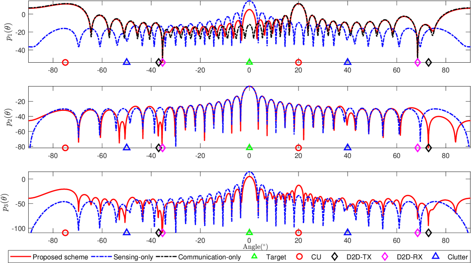
Finally, we evaluate the beampatterns at the BS when $\gamma_{r}=15\mathrm{dB}$, $P_{\text{BS}}=30$mW, and $P_{m}=10$mW. Fig. 8 shows the transmit beampattern $p_{1}(\theta)$, the receive beampattern $p_{2}(\theta)$, and the combined beampattern $p_{3}(\theta)$ where

References

- [1] F. Liu et al., “Integrated sensing and communications: Toward dual-functional wireless networks for 6G and beyond,” IEEE J. Sel. Areas Commun., vol. 40, no. 6, pp. 1728–1767, June 2022.
- [2] X. Fang, W. Feng, Y. Chen, N. Ge and Y. Zhang, “Joint communication and sensing toward 6G: Models and potential of using MIMO,” IEEE Internet Things J., vol. 10, no. 5, pp. 4093–4116, 1 Mar., 2023.
- [3] J. A. Zhang et al., “An overview of signal processing techniques for joint communication and radar sensing,” IEEE J. Sel. Topics Signal Process., vol. 15, no. 6, pp. 1295–1315, Nov. 2021.
- [4] Z. He, W. Xu, H. Shen, Y. Huang and H. Xiao, “Energy efficient beamforming optimization for integrated sensing and communication,” IEEE Wireless Commun. Lett., vol. 11, no. 7, pp. 1374–1378, July 2022.
- [5] Z. Wang, Y. Liu, X. Mu, Z. Ding and O. A. Dobre, “NOMA empowered integrated sensing and communication,” IEEE Commun. Lett., vol. 26, no. 3, pp. 677–681, Mar. 2022.
- [6] J. Li, G. Zhou, T. Gong and N. Liu, “Beamforming design for active IRS-aided MIMO integrated sensing and communication systems,” IEEE Wireless Commun. Lett., vol. 12, no. 10, pp. 1786–1790, Oct. 2023.
- [7] M. Hua, Q. Wu, W. Chen, O. A. Dobre and A. Lee Swindlehurst, “Secure intelligent reflecting surface aided integrated sensing and communication,” IEEE Trans. Wireless Commun., vol. 23, no. 1, pp. 575–591, Jan. 2024.
- [8] P. Liu, Z. Fei, X. Wang, B. Li, Y. Huang and Z. Zhang, “Outage constrained robust secure beamforming in integrated sensing and communication systems,” IEEE Wireless Commun. Lett., vol. 11, no. 11, pp. 2260–2264, Nov. 2022.
- [9] X. Liu, T. Huang, N. Shlezinger, Y. Liu, J. Zhou and Y. C. Eldar, ”Joint transmit beamforming for multiuser MIMO communications and MIMO radar,” IEEE Trans. Signal Process., vol. 68, pp. 3929–3944, 2020.
- [10] Z. Ren, L. Qiu, J. Xu and D. W. K. Ng, “Robust transmit beamforming for secure integrated sensing and communication,” IEEE Trans. Commun., vol. 71, no. 9, pp. 5549–5564, Sept. 2023.
- [11] M. Ashraf, B. Tan, D. Moltchanov, J. S. Thompson and M. Valkama, “Joint optimization of radar and communications performance in 6G cellular systems,” IEEE Trans. Green Commun. Netw., vol. 7, no. 1, pp. 522–536, March 2023.
- [12] Z. He, W. Xu, H. Shen, D. W. K. Ng, Y. C. Eldar and X. You, “Full-duplex communication for ISAC: Joint beamforming and power optimization,” IEEE J. Sel. Areas Commun., vol. 41, no. 9, pp. 2920–2936, Sept. 2023.
- [13] Z. Liu, S. Aditya, H. Li and B. Clerckx, “Joint transmit and receive beamforming design in full-duplex integrated sensing and communications,” IEEE J. Sel. Areas Commun., vol. 41, no. 9, pp. 2907–2919, Sept. 2023.
- [14] J. Chu, R. Liu, M. Li, Y. Liu and Q. Liu, “Joint secure transmit beamforming designs for integrated sensing and communication systems,” IEEE Trans. Veh. Technol., vol. 72, no. 4, pp. 4778–4791, Apr. 2023.
- [15] M. Lee, G. Yu and G. Y. Li, “Graph embedding based wireless link scheduling with few training samples”, IEEE Trans. Wireless Commun., vol. 20, no. 4, pp. 2282–2294, Apr. 2021.
- [16] S. S. Christensen, R. Agarwal, E. De Carvalho, and J. M. Cioffi, “Weighted sum-rate maximization using weighted MMSE for MIMO–BC beamforming design,” IEEE Trans. Wireless Commun., vol. 7, no. 12, pp. 4792–4799, Dec. 2008.
- [17] Q. Shi, M. Razaviyayn, Z. -Q. Luo and C. He, “An iteratively weighted MMSE approach to distributed sum-utility maximization for a MIMO interfering broadcast channel,” IEEE Trans. Signal Process., vol. 59, no. 9, pp. 4331–4340, Sept. 2011.
- [18] T. Chen, X. Zhang, M. You, G. Zheng and S. Lambotharan, “A GNN-based supervised learning framework for resource allocation in wireless IoT networks,” IEEE Internet Things J., vol. 9, no. 3, pp. 1712–1724, Feb. 2022.
- [19] Y. Gu, C. She, Z. Quan, C. Qiu and X. Xu, “Graph neural networks for distributed power allocation in wireless networks: Aggregation over-the-air,” IEEE Trans. Wireless Commun., vol. 22, no. 11, pp. 7551–7564, Nov. 2023.
- [20] X. Li, J. Zhang and X. Liu, “Mode selection and resource allocation for D2D communications with tradeoff of throughput and user satisfaction,” IEEE Trans. Commun., vol. 71, no. 9, pp. 5607–5620, Sept. 2023.
- [21] V. Vishnoi, I. Budhiraja, S. Gupta and N. Kumar, “A deep reinforcement learning scheme for sum rate and fairness maximization among D2D pairs underlaying cellular network with NOMA,” IEEE Trans. Veh. Technol., vol. 72, no. 10, pp. 13506–13522, Oct. 2023.
- [22] H. Xiao, D. Zhu and A. T. Chronopoulos, “Power allocation with energy efficiency optimization in cellular D2D-based V2X communication network,” IEEE Trans. Intell. Transp. Syst., vol. 21, no. 12, pp. 4947–4957, Dec. 2020.
- [23] Z. Yang, N. Huang, H. Xu, Y. Pan, Y. Li and M. Chen, “Downlink resource allocation and power control for device-to-device communication underlaying cellular networks,” IEEE Commun. Lett., vol. 20, no. 7, pp. 1449–1452, Jul. 2016.
- [24] N. Du, C. Zhou, H. Shen, C. Chakraborty, J. Yang and K. Yu, ”A novel power allocation algorithm for minimizing energy consumption in D2D communication systems,” IEEE Syst. J., vol. 17, no. 3, pp. 4969–4977, Sept. 2023.
- [25] J. Cheng, C. Shen, Z. Chen and N. Pappas, “Robust beamforming design for IRS-aided URLLC in D2D networks,” IEEE Trans. Commun., vol. 70, no. 9, pp. 6035–6049, Sept. 2022.
- [26] M. Lin, J. Ouyang and W. -P. Zhu, “Joint beamforming and power control for device-to-device communications underlaying cellular networks,” IEEE J. Sel. Areas Commun., vol. 34, no. 1, pp. 138–150, Jan. 2016.
- [27] W. Wang, L. Yang, A. Meng, Y. Zhan and D. W. K. Ng, “Resource allocation for IRS-aided JP-CoMP downlink cellular networks with underlaying D2D communications,” IEEE Trans. Wireless Commun., vol. 21, no. 6, pp. 4295–4309, June 2022.
- [28] B. ezbek, M. Pischella and D. Le Ruyet, “Energy efficient resource allocation for underlaying multi-D2D enabled multiple-antennas communications,” IEEE Trans. Veh. Technol., vol. 69, no. 6, pp. 6189–6199, June 2020.
- [29] Y. Chen et al., “Sub-channel allocation for full-duplex access and device-to-device links underlaying heterogeneous cellular networks using coalition formation games,” IEEE Trans. Veh. Technol., vol. 69, no. 9, pp. 9736–9749, Sept. 2020.
- [30] C. Wen, Y. Huang and T. N. Davidson, ”Efficient transceiver design for MIMO dual-function radar-communication systems,” IEEE Trans. Signal Process., vol. 71, pp. 1786–1801, 2023.
- [31] S. Boyd and L. Vandenberghe, Convex optimization. Cambridge, U.K.: Cambridge Univ. Press, 2004.
- [32] M. Grant and S. Boyd, “CVX: MATLAB software for disciplined convex programming”, Version 2.1. Accessed: Dec. 2018. [Online]. Available: http://cvxr.com/cvx
- [33] Z.-Q. Luo, W.-K. Ma, A. M.-C. So, Y. Ye and S. Zhang, “Semidefinite relaxation of quadratic optimization problems,” IEEE Signal Process. Mag., vol. 27, no. 3, pp. 20–34, May 2010.
- [34] A. Beck, A. Ben-Tal, and L. Tetruashvili, “A sequential parametric convex approximation method with applications to nonconvex truss topology design problems,” J. Global Optim., vol. 47, no. 1, pp. 29–51, May 2010.
- [35] Q. Qi, Y. Li and Q. Guo, “A bias-reduced solution for multistatic localization using differential delays and doppler shifts,” IEEE Trans. Aerosp. Electron. Syst., vol. 59, no. 5, pp. 5120–5133, Oct. 2023.
- [36] C. G. Tsinos, A. Arora, S. Chatzinotas and B. Ottersten, “Joint transmit waveform and receive filter design for dual-function radar-communication systems,” IEEE J. Sel. Topics Signal Process., vol. 15, no. 6, pp. 1378–1392, Nov. 2021.
- [37] M. Temiz, E. Alsusa and M. W. Baidas, “A dual-function massive MIMO uplink OFDM communication and radar architecture,” IEEE Trans. Cogn. Commun. Netw., vol. 8, no. 2, pp. 750–762, June 2022.
- [38] S.-H. Park and X. Jin, “Joint secure design of downlink and D2D cooperation strategies for multi-user systems,” IEEE Signal Process. Lett., vol. 28, pp. 917–921, 2021.
- [39] Q. Wu and R. Zhang, “Intelligent reflecting surface enhanced wireless network via joint active and passive beamforming,” IEEE Trans. Wireless Commun., vol. 18, no. 11, pp. 5394–5409, Nov. 2019.
- [40] Z. Lin et al., “Pain without gain: Destructive beamforming from a malicious RIS perspective in IoT networks,” IEEE Internet Things J., vol. 11, no. 5, pp. 7619–7629, Mar. 2024.
- [41] L. Wu, P. Babu and D. P. Palomar, “Transmit waveform/receive filter design for MIMO radar with multiple waveform constraints,” IEEE Trans. Signal Process., vol. 66, no. 6, pp. 1526–1540, Mar. 2018.
- [42] N. Su, F. Liu, Z. Wei, Y. -F. Liu and C. Masouros, ”Secure dual-functional radar-communication transmission: Exploiting interference for resilience against target eavesdropping,” IEEE Trans. Wireless Commun., vol. 21, no. 9, pp. 7238–7252, Sept. 2022.