Laboratory of Protein Design and Immunoengineering (LPDI), EPFL, Switzerland \alsoaffiliationNational Centre of Competence in Research (NCCR) Catalysis, EPFL, Switzerland
FSscore: A Personalized Machine Learning-based Synthetic Feasibility Score
S1 Code and data availability
All code used for training, fine-tuning, and scoring the FSscore is available at https://github.com/schwallergroup/fsscore. This repository also includes an application that can be run locally and allows a more intuitive and accessible way to label data, fine-tune, and deploy a model.
S1.1 Application
The application allows a user to perform all steps necessary to get a personalized model as intended. These steps involve: pairing molecules, labeling pairs, fine-tuning the pre-trained model, and ultimately scoring molecules. The application is built using Streamlit 1 but is deployed locally. This means that the speed is limited by the computer on which the user is running the app. All models were trained on one GPU (NVIDIA GeForce RTX 3090) but the application will run also on a computer without GPUs at the cost of a much increased running time. Furthermore, running it locally also requires the user to install the package, which we recommend doing using a conda environment and pip. All the necessary steps and usability are outlined below.
1. Installation
We recommend running the app with the packages stored in a conda environment111Conda installation guide: https://conda.io/projects/conda/en/latest/user-guide/install/index.html. First, clone the GitHub repository from the link above (alternatively download the zip file):
Next, change the directory to the repository and install all required packages, like so:
2. Start the application
Starting the application only requires one line of code (from the root directory of the repository), which will lead to a window to pop up or return an active link:
From the landing page, select Label molecules in the upper drop-down menu on the left. This will lead to selecting the next steps. If a dataset with labels is available, go to step 4., otherwise continue with the next step. To directly score molecules and a fine-tuned model is available one can jump to step 6.
3. Pair molecules
In this step, a list of molecules provided as SMILES first are paired, and then ranked based on uncertainty of the pre-trained model. This second step will take some time if not performed on a machine with GPU-support. Select the option on the left and provide the path to the csv file (Figure S1). This file should have smiles as a column header for the SMILES structures to be paired.

4. Label molecule pairs
If a dataset with paired molecules is available, place it in streamlit_app/data/unlabeled. The dataset should appear in the drop-down menu on the right. Make sure to provide the paired molecules with column headers smiles_i and smiles_j.
The labeling window (see Figure S2) prompts the user to select the molecule that is harder to synthesize, before going to the next pair. Once the user is finished labeling, the button Send labels can be pressed. The labeling process can also be continued later and the labeled data can be downloaded. Note: The more labeled pairs, the better the performance of the fine-tuned model.

5. Fine-tune
Once data is labeled, one can proceed to fine-tuning. This is by default done using the best pre-trained model from this work. The user can also place their own checkpoint at the same location (folder models). How to pre-train a new model is described on our GitHub repository. Before initializing fine-tuning, one can tune several hyperparameters. If nothing is adjusted, the (recommended) default parameters as used in this work are selected (Figure S3). Fine-tuning in general is very fast, but depending on your system this can take a few minutes. Proceeding to score molecules can be achieved by selecting the respective action on the upper drop-down menu. This process can cause some issues in which case we would recommend returning to the home page before trying again.

6. Score molecules
Lastly, one can deploy the previously fine-tuned model and score molecules. For this, the user may place a csv file in streamlit_app/data/scoring, which contains the column header smiles. Then, the user can select the correct dataset in the drop-down menu on the left as well as the desired fine-tuned model (Figure S4).

S2 Machine Learning Methods
The novel Focused Synthesizability score (FSscore) is trained in two stages. First, we train a baseline score assessing synthesizability using a graph representation and suitable message passing scheme improving expressivity over similar frameworks such as the SCScore. Secondly, we introduce our fine-tuning approach using human expert knowledge, allowing us to focus the score towards a specific chemical space of interest.
S2.1 Architecture and representation
Our approach to learning a continuous score to assess the synthesizability is inspired by Choung \latinet al. 2, which framed a similar task as a ranking problem using binary preferences. Specifically, every data point consists of two molecules for each of which we predict a scalar in separate forward passes. The minimization of the binary cross entropy between the true preference and the learned score difference (scaled using a sigmoid function) constitutes our training objective.
The function learns to parametrize molecules as an expressive latent representation given a set of molecules . We represent molecules as graphs with atoms as nodes and bonds as edges from which we can compute the line graph offline iteratively to the desired depth. The transformation process to the line graph is defined such that the edges of graph are the nodes of the line graph and these nodes are connected if the corresponding edges of share a node. The graph neural network (GNN) embedding the molecular graph consists of the graph attention network (GATv2) 3 operating on the graph and the Line Evolution (LineEvo) 4 layer operating on the line graph as message passing schemes. Both GATv2 and LineEvo use an attention mechanism to update the node representations as follows:
| (S1) |
where and are learned, denotes an activation function and denotes concatenation. The GNN operates on a hidden size of 128 and the input dimensions depend on the initial featurization of the edges and nodes (see Tab. S1. GATv2 layers use 8 heads and LeakyReLU as activation function after updating the hidden feature vector while LineEvo layers use ELU. In GATv2, these local attention scores are then averaged across all neighbors (see Eq. S2) to obtain a normalized attention coefficient to compute the updated node representation as a weighted average (see Eq. S3):
| (S2) |
| (S3) |
with PReLU 5 as nonlinearity . In LineEvo layers, is simply transformed using ELU to obtain the new node representation .
These transformation layers are stacked so that two GATv2 (G) layers are followed by one LineEvo (L) layer (GGLGGL). Each of these layers is followed by a readout function, which consists of a global max pooling layer and global weighted-add pooling as suggested by Ren \latinet al. 4 obtaining a molecular representation through concatenation of the two readouts. The intermediate molecular representations of all layers are summed, and the final score is inferred with a multilayer perceptron (MLP) (3 hidden layers of size 256, ReLU as activation function). The model described above was compared to five other implementations: GATv2 layers only (GGG) and four fingerprint implementations, namely Morgan (boolean), Morgan counts, Morgan chiral (boolean), and Morgan chiral counts, all with radius 4 and 2048 bits. 6 The fingerprints are embedded by one linear layer (hidden size of 256) with ReLU as activation function followed by the aforementioned MLP. More detailed information can be found in Section S2.3.
S2.2 Pairing molecules for fine-tuning
To focus our scoring model on a desired chemical space, we apply a fine-tuning approach inspired by Choung \latinet al. 2. This approach was optimized to require few data points in order to limit the time required from expert chemists labeling the training examples in case of labels based on human feedback. Datasets to be used for fine-tuning can be of various origins such as a chemical scope suggested by experimentalists or specific chemical spaces encompassing e.g. natural products. Training our model requires pairs of molecules with a binary preference as label. In order to do so, we first cluster a dataset using the k-means algorithm based on the Tanimoto distances of Morgan counts fingerprint. The number of clusters k was determined for every dataset individually where the mean Silhouette coefficient over a range of k was the smallest. 7. The range queried was set from 5 to 29 for datasets larger than 500 pairs and to 3 to 9 for smaller datasets. Secondly, molecules are paired in such a way that they come from different clusters, appear only once in the paired dataset and have opposite labels if available. We also investigated the influence of having overlapping pairs (molecules can appear multiple times) for the SYBA (CP and MC) and the meanComplexity datasets. This approach results in more fine-tuning data but does not satisfy our desire to keep the dataset size small since human labeling could not make use of this advantage. Subsequently, the uncertainty of the prediction of the pre-trained model on those pairs is determined based on the variance of obtained using the Monte Carlo dropout method 8 with a dropout rate of 0.2 on 100 predictions. The dataset is sorted with descending variance so that the pairs with high uncertainty are labeled first or used first for fine-tuning when selecting a subset. If no label is available the top n pairs (n depends on the dataset size) are submitted to be evaluated by our expert chemist based on their preference with regard to synthesizability.
S2.3 Training details
To center the obtained score around zero a regularization factor of 1e-4 was applied to the predicted score like to obtain the regularization loss as suggested by Choung \latinet al. 2. is added to the cross-entropy loss term as described in Section S2.1 to obtain the final loss .
Pre-training: The training set was randomly split in 25 equally sized subsets and the model was trained with each subset for 10 epochs totaling 250 epochs with a batch size of 128. This sequential learning approach was found to work well in increasing speed of training. The model was trained with the Adam optimizer 9 and an initial learning rate of 3e-4.
Fine-tuning: We chose a transfer learning type of fine-tuning where all the weights of the pre-trained model can get adapted. All the hyperparameter except learning rate and batch size are kept the same. In order to avoid the forgetting the previously learned we track the performance metrics on a random subset of 5,000 pairs from the hold-out test set of the pre-training data. Of the four tested initial learning rates (1e-5, 1e-4, 3e-4, 1e-3) we chose 1e-4 for the graph-based version and 3e-4 for the fingerprint-based models. These learning rates are a good trade-off between degradation of the previously learned and learning on the new dataset as can be seen in the learning curves in Appendix S6.1. We observed quick conversion with fewer than 20 epochs and in order to balance the aforementioned trade-off a custom early stopping method was applied. Training is stopped once either the validation loss (or training loss if the full dataset is used for production) has increased for 3 epochs (patience of 3) or the accuracy on the 5k subset of the hold-out test set decreased for 3 epochs with a delta threshold of 0.02. We trained for a maximum of 20 epochs. For evaluating the efficiency, we further varied the number of data points used for training of which we took 5 random pairs for validation. The results in Table S2 show improvement in performance the bigger the dataset size. The batch size was set to 4.
S2.4 Initial featurization of graphs
| Localization | Feature | Description | Size |
| atom | atom type | one-hot encoded atom type 222Considered atom types: [H, B, C, N, O, F, Si, P, S, Cl, Br, I, Se] | 14 |
| charge | one-hot encoded formal charge [-4,4] | 10 | |
| implicit hydrogens | one-hot encoded number of hydrogens [0,4] | 6 | |
| degree | one-hote encoded degree [0,4] | 6 | |
| ring information | 1 if in ring else 0 | 1 | |
| aromaticity | 1 if aromatic else 0 | 1 | |
| hybridization | one-hot encoded hybridization state 333Considered hybridization states: [UNSPECIFIED, s, sp, sp2, sp3, sp3d, sp3d2, other] | 9 | |
| chiral tag | one-hot encoded chiral tag [S, R, unassigned] | 4 | |
| bond type | one-hot encoded bond type 444Considered bond types: [single, double, triple, aromatic] | 5 | |
| bond | conjugated | 1 if conjugated else 0 | 1 |
| ring information | 1 if in ring else 0 | 1 |
S3 Data
S3.1 Pre-training data
To pre-train our model on a large collection of reactions, we combine the USPTO_full 11 patent dataset with a complementary dataset 12. Reaction data implicitly contains information on the synthetic feasibility through the relation of reactant to product, with the product being synthetically more difficult. The USPTO_full dataset was downloaded according to https://github.com/coleygroup/Graph2SMILES/blob/main/scripts/download_raw_data.py 13 using all USPTO_full subsets and "src" as product and "tgt" as reactants. The dataset was split so that every data point is a pair of one reactant and its respective product and the SMILES strings were canonicalized. The datasets do not contain reactions with multiple products. Data points with empty strings, identical reactants and products (isomeric SMILES), either reactant or product containing less than four heavy atoms or containing element types not in {H, B, C, N, O, F, Si, P, S, Cl, Se, Br, I} were removed. The datasets were further deduplicated retaining one instance of replicates. Furthermore, data points were removed ensuring that there are no cycles in the reaction network. This was achieved by removing back edges with the Depth-First Search (DFS) algorithm as implemented by Sun \latinet al. 14. The filtered dataset consisted of 5,340,704 data points. The train test split was performed so that no molecules (note not just reactant:product pairs) are overlapping resulting in a significant data loss to prevent data leakage. The training set consists of 3,349,455 pairs and the hold out test set of 711,550 pairs (17.5%).
To qualitatively evaluate the pre-trained model the performance on the MOSES 15 and COCONUT 16 dataset were assessed. We downloaded the MOSES test set from Polykovskiy \latinet al. 15 as is totaling 176,074 SMILES. COCONUT was extracted from Sorokina \latinet al. 16, all SMILES returning None with RDKit 10 were removed and a random subset of 176,000 molecules was selected to match the MOSES fraction.
S3.2 Fine-tuning data
The data for the fine-tuning case studies come from various sources. The specific processing steps for every dataset is outlined below.
Chirality: The obtain a test set for the chirality case study we filtered the deduplicated molecules from the pre-training training set keeping only those with @ or @@ tokens in the SMILES string, which define the chirality of a tetrahedral stereocenter. Of those, we sample 1,000 SMILES randomly and obtain their partner by getting the non-isomeric SMILES using RDKit rdk 10.
SYBA sets: The CP and MC test sets were extracted from Voršilák \latinet al. 17. No further processing was required.
meanComplexity: The meanComplexity dataset was downloaded from Sheridan \latinet al. 18 and cleaned by removing SMILES whose conversion to an RDKit molecule object failed. This processing step removed 44 SMILES yielding a fine-tuning test set of 1,731 molecules.
PROTACs: For the PROTAC case study we extracted all PROTAC SMILES from the PROTAC-DB Weng \latinet al. 19 and deduplicated the dataset keeping the first instance resulting in 3,270 SMILES. After pairing and ranking by confidence as described in Appendix S2.2, 100 pairs were labeled by a medicinal chemist with expertise in PROTACs. In order to compare the scores of the individual components to the full PROTAC as done in Figure LABEL:fig:protac_barplot the individual fragments (the two ligands and the linker) have to be extracted. For this, we extracted the collections containing information on anchor and warhead (the two ligands) from PROTAC-DB and tried to match an anchor and warhead to every PROTAC by matching protein target ID and find the biggest substructure match. The linker was obtained by removing the ligands’ atoms. For the 3270 PROTACs in the database we could find matching ligands for 1920 of them. This approach of extraction is necessary because PROTAC-DB does not cross-reference the PROTACs to the fragments and our extraction cannot guarantee concordance with the reported warhead and anchor in the respective publications but still is a good approximation.
S4 De novo design case study
To assess the applicability of the FSscore to a generative task we took advantage of the RL-framework of REINVENT 20 and used the recently proposed augmented memory 21 optimization protocol. First, an agent was trained with the composite (equal weights) of the docking score to the D2 Dopamine receptor (DRD2, PDB ID: 6CM4) and the molecular weight (MW) as a reward. The docking score was determined using AutoDock Vina 22 on one conformer each. Conformer generation is performed with RDKit 10 and the Universal force field (UFF) 23 for energy minimization for a maximum of 600 iterations. The score was scaled to obtain reward in a range of [0,1] by applying a sigmoid transformation as follows:
| (S4) |
with corresponding to a docking score of -1, -13 and the steepness was set to 0.25 resulting in a reverse sigmoid (a small docking score results in a reward towards 1 while a high score returns a reward close to 0). The score for MW was formulated so that a high reward is returned when having a MW between 0 and 500 Da using a double sigmoid like so:
| (S5) |
| (S6) |
| (S7) |
| (S8) |
| (S9) |
with coefficients and , the lower bound and upper bound . RL was carried out for 150 epochs, a batch size of 64, learning rate of 1e-4, a of 128 and augmented memory as optimization algorithm with 2 augmentation rounds and selective memory purge with a minimum similarity of 0.4 and a bin size of 10 based on the identical Murcko scaffold. For details on augmented memory in REINVENT we refer to Guo and Schwaller 21. For our first approach (FSscore optimization) all valid SMILES (9,246) generated during this optimization process were subsequently used to fine-tune the FSscore as described above. The agent already optimized for docking was next used to optimize for synthetic feasibility either with the fine-tuned FSscore or the SA score as a comparison. Both approaches were trained in identical fashion with the following parameters: 50 epochs, batch size of 128, of 128, a learning rate of 1e-4 and using the augmented memory algorithm with 2 rounds of augmentation. The diversity filter (incl. selective memory purge) was based on identical Murcko scaffolds based on a minimal similarity of 0.4, a minimal score of 0.4 and a bucket size of 25. The FSscore was transformed to range from 0 to 1 with a sigmoid according to Equation S4 with , and a steepness . The agent optimized for the SA score was transformed similarly reverting the sigmoid by setting , and . Thus, a high FSscore result in a high reward, while a low SA score results in high reward and vice versa. As mentioned above, only molecules with a minimal score of 0.4 were collected and subsequently used for evaluation. The second optimization approach using FSscore and the Chemspace API (FSscore + CS) was carried out similarly but instead of fine-tuning the FSscore once, the model was updated at every step for 50 rounds of RL. For all the valid and unique SMILES of each batch (max 128 molecules) the most similar molecule in the Chemspace database of buyable building blocks and buyable/synthesizable screening compounds (databases: CSSB, CSSS, CSMB, CSMS) were extracted and used as less difficult partner in a pair for the FSscore fine-tuning. Any data point was removed if an exact match was found. all other hyperparameters were chosen as outlined above. This yielded 4,779 SMILES from the FSscore-trained agent, 3,519 for the FSscore+CS-trained agent, and 4,915 SMILES from the SA score-trained agent. The results are compared by the number of reaction steps predicted by AiZynthFinder and the fraction of exact matches found in the Chemspace database. 24, 25
S5 Metrics
The Pearson correlation coefficient (PCC) between and is computed using the function scipy.stats.pearsonr 26 and is calculated as followed:
| (S10) |
with the mean of vector and the mean of vector y.
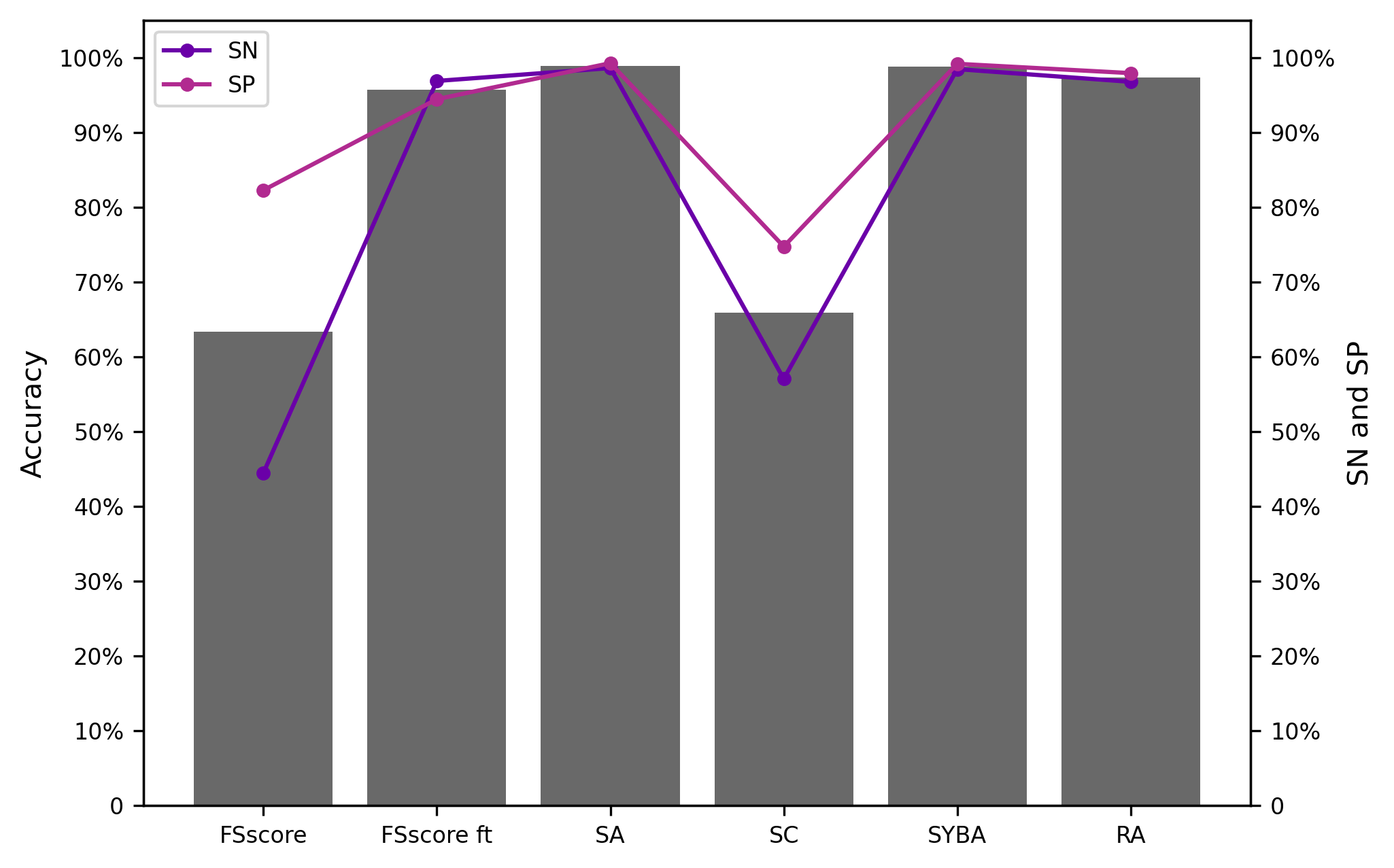
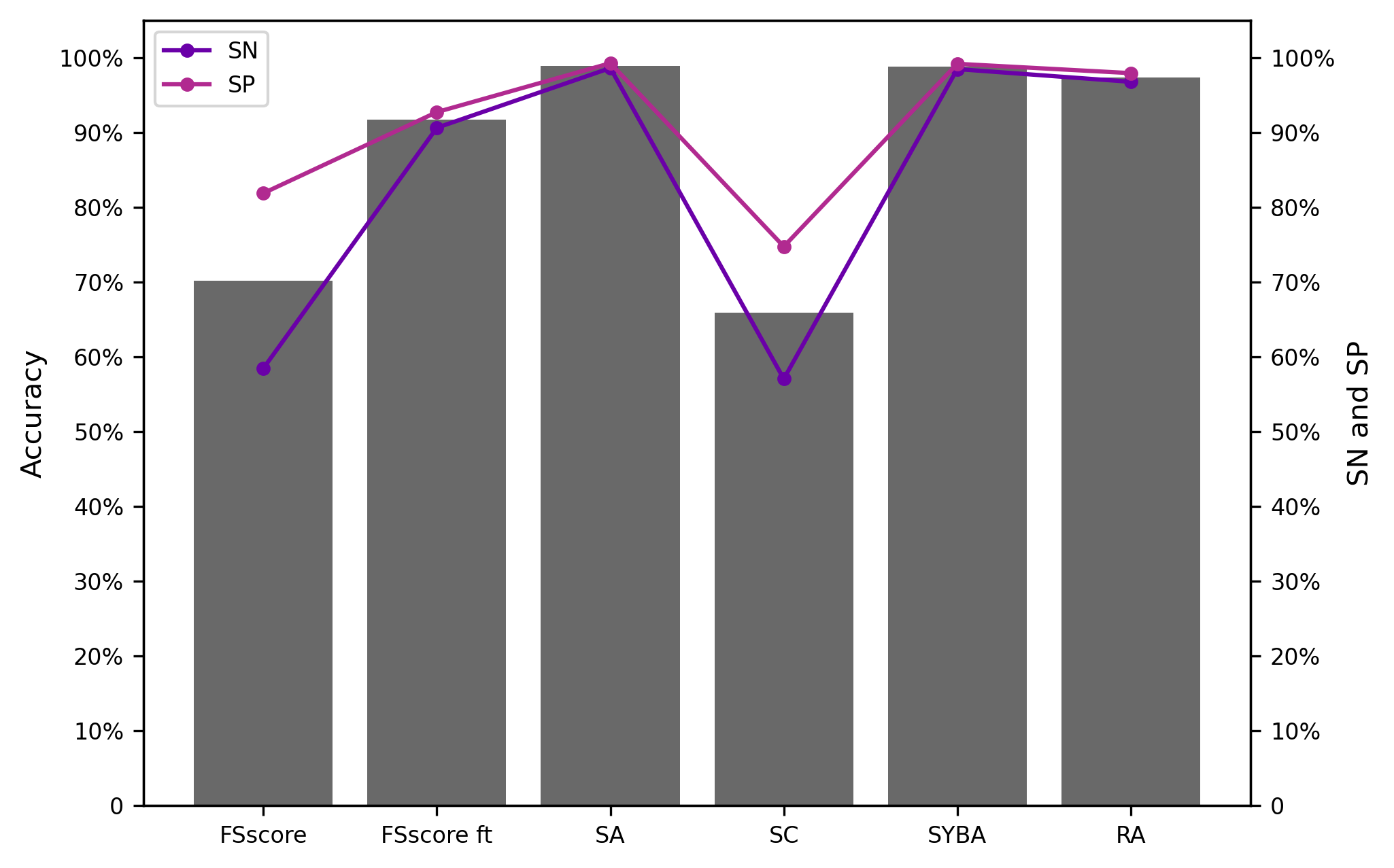
The following metrics for datasets with binary labels (e.g. HS \latinvs. ES) are computed using the sklearn.metrics package 27. Accuracy (Acc), sensitivity (SN) and specificity are calculated based on the relative sizes of true positives (TP), true negatives (TN), false positives (FP) and false negatives (FN):
| (S11) |
| (S12) |
| (S13) |
The area under the receiver operating characteristic (ROC) curve (AUC) describes the ability to discriminate data points based on binary labels at various thresholds. It is computed by plotting SN against at various cut-off values defining the two classes.
S6 Additional results


S6.1 SYBA test sets
| set | mode | |||||
|---|---|---|---|---|---|---|
| chiral | graph | no FT | 0.5435 | 0.5391 | 0.905 | 0.971 |
| 20 | 0.5762 (0.575) | 0.5972 (0.5947) | 0.9044 | 0.9706 | ||
| 30 | 0.5918 (0.592) | 0.6185 (0.6173) | 0.9035 | 0.97 | ||
| 40 | 0.6156 (0.6145) | 0.6539 (0.6521) | 0.9022 | 0.9692 | ||
| 50 | 0.6268 (0.6235) | 0.6749 (0.6728) | 0.8983 | 0.9671 | ||
| fp | no FT | 0.509 | 0.4989 | 0.875 | 0.957 | |
| 20 | 0.5163 (0.5165) | 0.5082 (0.5102) | 0.879 | 0.959 | ||
| 30 | 0.5180 (0.5195) | 0.5122 (0.5153) | 0.8786 | 0.9583 | ||
| 40 | 0.5255 (0.5255) | 0.5180 (0.5212) | 0.8738 | 0.9544 | ||
| 50 | 0.5237 (0.5235) | 0.5147 (0.5174) | 0.8783 | 0.9582 | ||
| CP 17 | graph | no FT | 0.6319 | 0.6446 | 0.905 | 0.971 |
| 20 | 0.9275 (0.9273) | 0.9804 (0.9802) | 0.903 | 0.9700 | ||
| 30 | 0.943 (0.9429) | 0.9868 (0.9865) | 0.9021 | 0.9695 | ||
| 40 | 0.9592 (0.9587) | 0.9933 (0.9930) | 0.9012 | 0.9689 | ||
| 50 | 0.9567 (0.9560) | 0.9921 (0.9918) | 0.9008 | 0.9687 | ||
| fp | no FT | 0.7008 | 0.7566 | 0.880 | 0.959 | |
| 20 | 0.8683 (0.8685) | 0.9396 (0.9397) | 0.8771 | 0.9568 | ||
| 30 | 0.8833 (0.8838) | 0.9517 (0.9521) | 0.8741 | 0.9543 | ||
| 40 | 0.9043 (0.9045) | 0.9645 (0.9649) | 0.8732 | 0.9536 | ||
| 50 | 0.9167 (0.9178) | 0.9725 (0.9731) | 0.8708 | 0.952 | ||
| MC 17 | graph | no FT | 0.5375 | 0.4894 | 0.905 | 0.971 |
| 20 | 0.65 (0.7875) | 0.645 (0.7744) | 0.9034 | 0.9695 | ||
| 30 | 0.6 (0.7625) | 0.55 (0.8150) | 0.9034 | 0.9696 | ||
| 40 | (0.85) | (0.906) | 0.8998 | 0.9679 | ||
| fp | no FT | 0.5875 | 0.515 | 0.880 | 0.959 | |
| 20 | 0.6 (0.7125) | 0.5425 (0.7832) | 0.8820 | 0.9596 | ||
| 30 | 0.7 (0.8875) | 0.61 (0.8994) | 0.8734 | 0.9529 | ||
| 40 | (0.825) | (0.8513) | 0.8786 | 0.9579 | ||
| PROTAC-DB 19 | graph | no FT | 0.53 | 0.4341 | 0.905 | 0.971 |
| 20 | 0.5063 (0.515) | 0.4341 (0.4602) | 0.905 | 0.9715 | ||
| 30 | 0.5214 (0.555) | 0.4587 (0.5474) | 0.9023 | 0.9697 | ||
| 40 | 0.5083 (0.51) | 0.4583 (0.4781) | 0.9048 | 0.9712 | ||
| 50 | 0.57 (0.6) | 0.522 (0.6142) | 0.8993 | 0.968 | ||
| 60 | 0.55 (0.615) | 0.5097 (0.6389) | 0.8984 | 0.9672 | ||
| 70 | 0.5167 (0.675) | 0.4433 (0.6857) | 0.8954 | 0.9659 | ||
| 80 | 0.55 (0.685) | 0.4725 (0.7281) | 0.8975 | 0.9672 | ||
| generated | graph | no FT | 0.5594 | 0.5255 | 0.905 | 0.971 |
| 20 | 0.5741 (0.5842) | 0.5437 (0.5629) | 0.8971 | 0.9675 | ||
| 30 | 0.5775 (0.6139) | 0.5444 (0.6117) | 0.8969 | 0.9673 | ||
| 40 | 0.5656 (0.6535) | 0.5612 (0.6686) | 0.8942 | 0.9659 | ||
| 50 | 0.5882 (0.604) | 0.5692 (0.589) | 0.9012 | 0.9694 | ||
| 60 | 0.5823 (0.6485) | 0.5756 (0.6566) | 0.8887 | 0.9632 | ||
| 70 | 0.6034 (0.6287) | 0.6177 (0.6527) | 0.8907 | 0.9643 | ||
| 80 | 0.6316 (0.7376) | 0.6357 (0.7752) | 0.8847 | 0.9616 |
| set | mode | ||||||
| CP 17 | graph | no FT | 7162 | 0.6319 | 0.6446 | 0.905 | 0.971 |
| 20 | 7122 | 0.8869 (0.8869) | 0.9543 (0.9544) | 0.9037 | 0.9639 | ||
| 50 | 7062 | 0.9598 (0.9598) | 0.9933 (0.9933) | 0.9008 | 0.9622 | ||
| 100 | 6962 | 0.9779 (0.9779) | 0.9978 (0.9978) | 0.8984 | 0.9609 | ||
| 500 | 6162 | 0.9982 (0.9982) | 1.0 (1.0) | 0.8773 | 0.9469 | ||
| 1000 | 5163 | 0.9983 (0.9983) | 1.0 (1.0) | 0.8662 | 0.941 | ||
| 2000 | 3371 | 0.9990 (0.9990) | 1.0 (1.0) | 0.8497 | 0.9318 | ||
| fp | no FT | 7162 | 0.7008 | 0.7566 | 0.880 | 0.959 | |
| 20 | 7122 | 0.8489 (0.8489) | 0.9201 (0.9207) | 0.8761 | 0.9471 | ||
| 50 | 7062 | 0.8833 (0.8830) | 0.9517 (0.9487) | 0.8721 | 0.944 | ||
| 100 | 6962 | 0.9102 (0.9102) | 0.9679 (0.9689) | 0.8688 | 0.9403 | ||
| 500 | 6162 | 0.9789 (0.9789) | 0.9970 (0.9974) | 0.8564 | 0.9285 | ||
| 1000 | 5164 | 0.9901 (0.9901) | 0.9989 (0.9993) | 0.8415 | 0.9168 | ||
| 2000 | 3372 | 0.9965 (0.9965) | 0.9997 (0.9999) | 0.8179 | 0.8981 | ||
| MC 17 | graph | no FT | 80 | 0.5375 | 0.4894 | 0.905 | 0.971 |
| 20 | 59 | 0.6625 (0.6625) | 0.5829 (0.6656) | 0.8985 | 0.9607 | ||
| 50 | 41 | 0.775 (0.775) | 0.7273 (0.8175) | 0.8971 | 0.9593 | ||
| 100 | 32 | 0.8125 (0.8125) | 0.8155 (0.8244) | 0.8995 | 0.9609 | ||
| 500 | 20 | 0.9 (0.9) | 0.6813 (0.9375) | 0.8698 | 0.9414 | ||
| fp | no FT | 80 | 0.5875 | 0.515 | 0.880 | 0.959 | |
| 20 | 60 | 0.6375 (0.6375) | 0.4733 (0.6313) | 0.8797 | 0.9502 | ||
| 50 | 44 | 0.85 (0.85) | 0.7789 (0.9106) | 0.8669 | 0.9415 | ||
| 100 | 29 | 0.925 (0.9250) | 0.8389 (0.9484) | 0.8545 | 0.9312 | ||
| 500 | 20 | 0.95 (0.95) | 0.8542 (0.9612) | 0.8324 | 0.9118 |
S6.1.1 CP test set


S6.1.2 MC test set


S6.2 meanComplexity dataset
| dataset | unique | mode | PCC | ||||
|---|---|---|---|---|---|---|---|
| meanComplexity 18 | yes | graph | no FT | 1681 | 0.51 | 0.905 | 0.971 |
| 20 | 1641 | 0.61 | 0.9034 | 0.9701 | |||
| 30 | 1621 | 0.63 | 0.9035 | 0.9697 | |||
| 40 | 1601 | 0.66 | 0.9033 | 0.9697 | |||
| 50 | 1581 | 0.66 | 0.9028 | 0.9689 | |||
| fp | no FT | 1681 | 0.49 | 0.880 | 0.959 | ||
| 20 | 1641 | 0.58 | 0.8768 | 0.9569 | |||
| 30 | 1621 | 0.68 | 0.8668 | 0.9492 | |||
| 40 | 1601 | 0.68 | 0.8483 | 0.9353 | |||
| 50 | 1581 | 0.67 | 0.8674 | 0.9502 | |||
| no | graph | no FT | 1681 | 0.51 | 0.905 | 0.971 | |
| 20 | 1649 | 0.55 | 0.8995 | 0.9615 | |||
| 50 | 1582 | 0.51 | 0.9017 | 0.963 | |||
| 100 | 1552 | 0.73 | 0.8921 | 0.9564 | |||
| 500 | 1291 | 0.84 | 0.8765 | 0.9447 | |||
| fp | no FT | 1681 | 0.49 | 0.880 | 0.959 | ||
| 20 | 1648 | 0.51 | 0.8809 | 0.9513 | |||
| 50 | 1584 | 0.59 | 0.8763 | 0.9475 | |||
| 100 | 1538 | 0.7 | 0.8632 | 0.9377 | |||
| 500 | 1292 | 0.8 | 0.8412 | 0.9212 |


S7 Example structures
S7.1 Hold-out test set


S7.2 CP and MC test sets


S7.3 PROTAC-DB


S7.4 REINVENT case study

S8 Learning curves


References
- 1 Streamlit. https://streamlit.io
- Choung \latinet al. 2023 Choung, O.-H.; Vianello, R.; Segler, M.; Stiefl, N.; Jiménez-Luna, J. Learning chemical intuition from humans in the loop. 2023; https://chemrxiv.org/engage/chemrxiv/article-details/63f89282897b18336f0c5a55
- Brody \latinet al. 2022 Brody, S.; Alon, U.; Yahav, E. How Attentive are Graph Attention Networks? International Conference on Learning Representations. 2022
- Ren \latinet al. 2023 Ren, G.-P.; Wu, K.-J.; He, Y. Enhancing Molecular Representations Via Graph Transformation Layers. Journal of Chemical Information and Modeling 2023, Publisher: American Chemical Society
- He \latinet al. 2015 He, K.; Zhang, X.; Ren, S.; Sun, J. Delving deep into rectifiers: Surpassing human-level performance on imagenet classification. Proceedings of the IEEE international conference on computer vision. 2015; pp 1026–1034
- Rogers and Hahn 2010 Rogers, D.; Hahn, M. Extended-connectivity fingerprints. Journal of chemical information and modeling 2010, 50, 742–754
- Rousseeuw 1987 Rousseeuw, P. J. Silhouettes: A graphical aid to the interpretation and validation of cluster analysis. Journal of Computational and Applied Mathematics 1987, 20, 53–65
- Gal and Ghahramani 2016 Gal, Y.; Ghahramani, Z. Dropout as a bayesian approximation: Representing model uncertainty in deep learning. international conference on machine learning. 2016; pp 1050–1059
- Kingma and Ba 2014 Kingma, D. P.; Ba, J. Adam: A method for stochastic optimization. arXiv preprint arXiv:1412.6980 2014,
- 10 RDKit: Open-source cheminformatics. http://www.rdkit.org
- Lowe 2012 Lowe, D. M. Extraction of chemical structures and reactions from the literature. Ph.D. thesis, University of Cambridge, 2012
- Jiang \latinet al. 2021 Jiang, S.; Zhang, Z.; Zhao, H.; Li, J.; Yang, Y.; Lu, B.-L.; Xia, N. When SMILES Smiles, Practicality Judgment and Yield Prediction of Chemical Reaction via Deep Chemical Language Processing. IEEE Access 2021, 9, 85071–85083, Conference Name: IEEE Access
- Tu and Coley 2022 Tu, Z.; Coley, C. W. Permutation Invariant Graph-to-Sequence Model for Template-Free Retrosynthesis and Reaction Prediction. Journal of Chemical Information and Modeling 2022, 62, 3503–3513, Publisher: American Chemical Society
- Sun \latinet al. 2017 Sun, J.; Ajwani, D.; Nicholson, P. K.; Sala, A.; Parthasarathy, S. Breaking cycles in noisy hierarchies. Proceedings of the 2017 ACM on Web Science Conference. 2017; pp 151–160
- Polykovskiy \latinet al. 2020 Polykovskiy, D.; Zhebrak, A.; Sanchez-Lengeling, B.; Golovanov, S.; Tatanov, O.; Belyaev, S.; Kurbanov, R.; Artamonov, A.; Aladinskiy, V.; Veselov, M.; Kadurin, A.; Johansson, S.; Chen, H.; Nikolenko, S.; Aspuru-Guzik, A.; Zhavoronkov, A. Molecular Sets (MOSES): A Benchmarking Platform for Molecular Generation Models. Frontiers in Pharmacology 2020, 11
- Sorokina \latinet al. 2021 Sorokina, M.; Merseburger, P.; Rajan, K.; Yirik, M. A.; Steinbeck, C. COCONUT online: Collection of Open Natural Products database. Journal of Cheminformatics 2021, 13, 2
- Voršilák \latinet al. 2020 Voršilák, M.; Kolář, M.; Čmelo, I.; Svozil, D. SYBA: Bayesian estimation of synthetic accessibility of organic compounds. Journal of Cheminformatics 2020, 12, 35
- Sheridan \latinet al. 2014 Sheridan, R. P.; Zorn, N.; Sherer, E. C.; Campeau, L.-C.; Chang, C. Z.; Cumming, J.; Maddess, M. L.; Nantermet, P. G.; Sinz, C. J.; O’Shea, P. D. Modeling a Crowdsourced Definition of Molecular Complexity. Journal of Chemical Information and Modeling 2014, 54, 1604–1616, Publisher: American Chemical Society
- Weng \latinet al. 2022 Weng, G.; Cai, X.; Cao, D.; Du, H.; Shen, C.; Deng, Y.; He, Q.; Yang, B.; Li, D.; Hou, T. PROTAC-DB 2.0: an updated database of PROTACs. Nucleic Acids Research 2022, gkac946
- Blaschke \latinet al. 2020 Blaschke, T.; Arús-Pous, J.; Chen, H.; Margreitter, C.; Tyrchan, C.; Engkvist, O.; Papadopoulos, K.; Patronov, A. REINVENT 2.0: An AI Tool for De Novo Drug Design. Journal of Chemical Information and Modeling 2020, 60, 5918–5922, Publisher: American Chemical Society
- Guo and Schwaller 2023 Guo, J.; Schwaller, P. Augmented Memory: Capitalizing on Experience Replay to Accelerate De Novo Molecular Design. 2023; http://arxiv.org/abs/2305.16160, arXiv:2305.16160 [cs, q-bio]
- Koes \latinet al. 2013 Koes, D. R.; Baumgartner, M. P.; Camacho, C. J. Lessons Learned in Empirical Scoring with smina from the CSAR 2011 Benchmarking Exercise. Journal of Chemical Information and Modeling 2013, 53, 1893–1904, Publisher: American Chemical Society
- Rappe \latinet al. 1992 Rappe, A. K.; Casewit, C. J.; Colwell, K. S.; Goddard, W. A. I.; Skiff, W. M. UFF, a full periodic table force field for molecular mechanics and molecular dynamics simulations. Journal of the American Chemical Society 1992, 114, 10024–10035, Publisher: American Chemical Society
- Genheden \latinet al. 2020 Genheden, S.; Thakkar, A.; Chadimová, V.; Reymond, J.-L.; Engkvist, O.; Bjerrum, E. AiZynthFinder: a fast, robust and flexible open-source software for retrosynthetic planning. Journal of Cheminformatics 2020, 12, 70
- 25 Chemspace search. https://chem-space.com/search
- Virtanen \latinet al. 2020 Virtanen, P.; Gommers, R.; Oliphant, T. E.; Haberland, M.; Reddy, T.; Cournapeau, D.; Burovski, E.; Peterson, P.; Weckesser, W.; Bright, J.; van der Walt, S. J.; Brett, M.; Wilson, J.; Millman, K. J.; Mayorov, N.; Nelson, A. R. J.; Jones, E.; Kern, R.; Larson, E.; Carey, C. J.; Polat, İ.; Feng, Y.; Moore, E. W.; VanderPlas, J.; Laxalde, D.; Perktold, J.; Cimrman, R.; Henriksen, I.; Quintero, E. A.; Harris, C. R.; Archibald, A. M.; Ribeiro, A. H.; Pedregosa, F.; van Mulbregt, P.; SciPy 1.0 Contributors SciPy 1.0: Fundamental Algorithms for Scientific Computing in Python. Nature Methods 2020, 17, 261–272
- Buitinck \latinet al. 2013 Buitinck, L.; Louppe, G.; Blondel, M.; Pedregosa, F.; Mueller, A.; Grisel, O.; Niculae, V.; Prettenhofer, P.; Gramfort, A.; Grobler, J.; Layton, R.; VanderPlas, J.; Joly, A.; Holt, B.; Varoquaux, G. API design for machine learning software: experiences from the scikit-learn project. ECML PKDD Workshop: Languages for Data Mining and Machine Learning. 2013; pp 108–122