FSNet: Redesign Self-Supervised MonoDepth for Full-Scale Depth Prediction for Autonomous Driving
Abstract
Predicting accurate depth with monocular images is important for low-cost robotic applications and autonomous driving. This study proposes a comprehensive self-supervised framework for accurate scale-aware depth prediction on autonomous driving scenes utilizing inter-frame poses obtained from inertial measurements. In particular, we introduce a Full-Scale depth prediction network named FSNet. FSNet contains four important improvements over existing self-supervised models: (1) a multichannel output representation for stable training of depth prediction in driving scenarios, (2) an optical-flow-based mask designed for dynamic object removal, (3) a self-distillation training strategy to augment the training process, and (4) an optimization-based post-processing algorithm in test time, fusing the results from visual odometry. With this framework, robots and vehicles with only one well-calibrated camera can collect sequences of training image frames and camera poses, and infer accurate 3D depths of the environment without extra labeling work or 3D data. Extensive experiments on the KITTI dataset, KITTI-360 dataset and the nuScenes dataset demonstrate the potential of FSNet. More visualizations are presented in https://sites.google.com/view/fsnet/home
Note to Practitioners
This paper was motivated by the problem of unsupervised monocular depth for robotic deployment. We notice that PoseNet is not generalizable and by nature monodepth2 only predict depths up to a scale. We believe that we should not expect PoseNet, a ResNet on a concatenation of two images, to produce more reliable poses than the localization module in a robot. So we try our best to completely avoid using PoseNet. This creates much unstability in training, but we managed to fix it in FSNet with multichannel output and self-distillation. We also believe the network should try to directly predict accurate depth with a correct scale at any cases. So our method could produce meaningful results on static frames or scenes with little/no VO points (same as the network’s direct prediction). There are images without VO points in our multi-frame experiment, but our method is robust enough to fix this problem. In future research, we will include multi-frame depth predictions for more accurate depth prediction.
Index Terms:
Autonomous Driving, Depth Prediction, Computer Vision.I Introduction
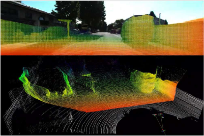
Dense depth prediction from a single RGB image is a significant challenge in computer vision and is useful in the robotics community. Though active sensors like LiDAR can directly produce accurate depth measurements of the environment, camera-based setups are still popular because cameras are relatively cheap, power-efficient, and flexible in that they can be mounted on various robotic platforms. Thus, monocular depth prediction enables more sophisticated 3D perception and planning tasks for many camera-based robots and low-cost self-driving setups [1, 2, 3], also including products like Tesla’s FSD and Valeo’s vision-only system [4]. A qualitative prediction sample of our work is presented in Figure 1, showing the potential of directly perceiving the world in 3D with a monocular camera.
Efficiently deploying a monocular depth prediction network in a new environment raises challenges for existing methods. As pretrained vision models do not usually generalize well enough to new scenes or a new camera setup [5], it is extremely useful and convenient to directly train a depth estimation model using raw data collected from the deployed robot in the target environment. However, most of the current self-supervised monocular depth using only monocular image sequences can only provide depth prediction with an ambiguity in the global scale of the depth results unless using stereo images [6, 7, 8, 9] or external point clouds supervision in training [10].
A mobile robotic system or a self-driving car usually produces a robot’s pose online by a standalone localization module. Moreover, with onboard sensors like the inertial measurement unit (IMU) and wheel encoder, the localization module can produce accurate relative poses between consecutive keyframes. Thus, we focus on the usage of poses to tackle scale ambiguity so that the network can be trained to predict depths with correct global scales.
In this paper, we develop the FSNet framework step by step from the use of pose. First, we investigate the training process of the unsupervised MonoDepth and demonstrate why directly replacing the output from PoseNet [6] with real camera poses will cause failure in training. This justifies the multichannel output representation adopted in our paper. Then, the availability of poses enables the computation of optical-flow-based masks for dynamic object removal. Moreover, we introduce a self-distillation framework to help stabilize the training process and improve final prediction accuracy. Finally, to use historical poses in test time, we introduce an optimization-based post-processing algorithm that uses sparse 3D points from visual odometry (VO) to improve the test time performance and enhance the robustness to changes in the extrinsic parameters of the robot. The main contributions of the paper are as follows:
-
•
An investigation of the training process of the baseline unsupervised monocular depth prediction networks. A multichannel output representation enables stable network training with full-scale depth output.
-
•
An optical-flow-based mask for dynamic object removal inspired by the introduction of inter-frame poses.
-
•
A self-distillation training strategy with aligned scales to improve the model performance while not introducing additional test-time costs.
-
•
An efficient post-processing algorithm that fuses the full-scale depth prediction and sparse 3D points predicted by visual odometry to improve test-time depth accuracy.
- •
The remainder of this paper is organized as follows: Section II reviews related work. Section III introduces our FSNet. Section IV presents the experimental results and compares our framework with existing self-supervised monocular depth prediction frameworks. Section V presents ablation studies and discussions on the components proposed in the paper. Finally, we conclude this paper in the last section.
II Related Works
II-A Self-Supervised Monocular Depth Prediction
Monodepth2 [6] sets up the baseline framework for self-supervised monocular depth prediction. The core idea of the training of Monodepth2 is to teach the network to predict dense depths that reconstruct the target image from source views. ManyDepth [7] utilizes the geometry in the matching between temporal images to improve the accuracy of single image depth prediction. However, the cost volume construction slows the inference speed and makes it difficult to accelerate on robotics platforms.
To obtain the correct scale directly from monocular depth prediction, researchers use either LiDAR [14, 10, 15] or stereo cameras [8, 9, 16, 17, 18] to provide supervision. Among stereo methods, Depth Hints [8], and Wavelet Depth [9] use traditional stereo matching algorithms to provide direct supervision to the depth prediction network. Monorec [16] uses stereo images to provide scale for the network and to identify moving object pixels in the sequence. DNet [19] uses the ground plane estimated from the normal of the image to calibrate the global scale of the predicted depth, but it fails in the nuScenes dataset which contains many image frames without a clear ground plane.
Our proposed FSNet uses poses from robots to regularize the network to predict correct scales without requiring a multiview camera or LiDARs. We point out that relative poses between frames are commonly available for robotic platforms because of sensors like IMUs and wheel encoders.

II-B Knowledge Distillation
Knowledge distillation (KD) is a field of pioneering training methods that transfers knowledge from teacher models to target student models [20]. KD has been applied in various tasks, including image classification [21], object detection [22, 23], and incremental learning [24]. The philosophy of knowledge distillation is training a small target model with an additional loss function to mimic the output of a teacher model. The teacher network could be an ensemble of the target models [25], a larger network [26], or a model with additional information inputs or different sensors [27].
Self-distillation (SD) is a special case where the teacher model is completely identical to the student model, and no additional input is applied to train the teacher model. Some existing works have demonstrated its performance on image classification [28].
In this paper, we first investigate the training process of an unsupervised monocular depth predictor, then we apply an offline-SD to our proposed model to regularize the training process and improve the final performance.
II-C Visual Odometry
Visual odometry (VO) systems [29, 30, 31] are widely used to provide robot centric pose information for autonomous navigation [32] and simultaneously estimate the ego-motion of the camera and the position of 3D landmarks. With IMU or Global navigation satellite system (GNSS) information, the absolute scale of the estimations can also be recovered [33, 34].
ORB-SLAM3 [31] is a typical indirect VO method in which the current input frame is tracked online with a 3D landmark map built incrementally. In this tracking process, the local features extracted are first associated with landmarks on the map. Then, the camera pose and correspondences are estimated within a Perspective-n-Point scheme. The depth of the local feature point can be retrieved from the associated 3D landmark and the camera pose, yielding an image-aligned sparse depth map for each frame. In this work, we use these sparse depth maps as an input for the full-scale dense depth prediction post-optimization procedure.
II-D Monocular Depth Completion
Monocular depth completion means predicting a dense depth with a monocular image and sparse ground truth LiDAR points. Learning-based methods usually follow the scheme of partial differential equations (PQEs) that extrapolate depth between sparse points based on the constraints learned from RGB pixels [35]. Other new methods without deep learning or extra ground truth labels exist. IPBasic [36] produces dense depth with morphological operations. Bryan et al. [37] introduce superpixel segmentation to segment images into different units, and each unit is considered as a plane or a convex hull.
In our proposed post-processing step, the merging between dense network depth prediction and visual odometry can be formulated into the same optimization problem as monocular depth completion but with extra uncertainty and hints. The proposed method is formulated without extra LiDAR point labels.
III MonoDepth2 Review
We first review the pipeline of MonoDepth2. The target is to train a model mapping the input target image frame to a dense depth map , with reconstruction supervision from neighboring frames. The depth is decoded from the convolutional output as
| (1) |
where and are hyper-parameters for the boundary of the depth prediction.
The depth map is reprojected to neighboring source keyframes with pose predicted from PoseNet. Then, the target frame is reconstructed using colors sampled from neighboring source frames and produces where . The photometric loss is the weighted sum of the structural similarity index measure (SSIM) and the L1 difference between the two images. The loss is expressed as:
| (2) |
where measures the structural difference between the two images using a kernel, and and is a constant with value 0.85 and 0.15, following [6].
As shown in our-own experiments and [38], directly substituting PoseNet with poses from the localization module will cause failure in training the network. We notice that the baseline depth decoder method will produce corrupted reconstruction results at initialization if directly fed with the correct pose. We need to take additional measures to preserve organic reconstruction results during the start of the training.
IV Methods
In order to stably train the depth prediction network with inter-frame poses, we reformulate the output of MonoDepth2 as multi-channel outputs. Inter-frame poses are further utilized to filter out dynamic objects during training with an optical flow-based mask. The overall system pipeline is presented in Fig 2.
IV-A Output Modification From MonoDepth2
Multichannel Output: In order to preserve organic reconstruction results, we select reformulate the output as multi-channel outputs, to allow larger depth values during initialization and also unsaturated gradients at large depth values.
Assuming the predicted depth should be within and the output is decoded from channels of the output network, then is defined as the proportion between consecutive depth bins, and the th bin will represent . Considering the softmax activated output of the network being , we interpret the weighted mean of each depth bin as the predicted depth .
At initialization, the network will predict an almost-uniform distribution for each depth bin, so the initial decoded depth will be the algorithmic mean of the depth bins . To guide the selection of hyperparameters, we analyze the initial depth values in our framework.
Theorem : The algorithmic mean of a proportional array, bounded by will converge to the following limit as the number of bins grows:
| (3) |
Proof: Denote the boundary of the predicted depth as , the th bins will represent . As presented in the paper, the initial depth predicted by the network will be the mean of all depth bins .
The mean of the proportional array will be
| (4) | ||||
L’Hôpital’s rule is applied at to obtain the final result.
We set for the autonomous driving scene. Based on (4), we choose for our network to obtain to ensure stable training initialization.
Camera-Aware Depth Adaption: To train one single depth prediction network on all six cameras of the nuScenes dataset, we point out that we need to take the difference of camera intrinsic matrix into account. Similar object appearance produces similar features in the network, while depth predictions should vary based on the focal length of the camera. As a result, we adapt the value of the depth bins according to the input camera as , where is a hyper-parameter chosen according to the front camera in nuScenes.
IV-B Optical Flow Mask
With the introduction of ego-vehicle poses at training times, we have a stronger prior for dynamic object removal. We know that the reprojection of a static 3D point on neighboring frames must stay on an epipolar line regardless of the distance between that point to the camera. The epipolar line can be computed as a vector with a length of three , where are the the coordinate of the pixel in the base frame and is the fundamental matrix between the two frame. The fundamental matrix is further calculated from , with camera intrinsics parameters , and relative pose between two image frames.
Therefore, if the reprojected point was far from its epipolar line, we can estimate that this point is probably related to a dynamic object and should probably be omitted during training loss computation.
To construct the optical flow mask for dynamic object removal, we first compute the optical flow between the two image frames using a pretrained unsupervised optical flow estimator ArFlow [39]. The distance between the reprojected point from the epipolar line is computed as with
| (5) |
where represents the first and second element of vector . Pixels with a deviation larger than 10 pixels are considered dynamic pixels. In this way, we produce a loss mask for photometric reconstruction loss computation.
IV-C Self-Distillation
As discussed in Section III, the monocular depth prediction network starts training with a generally uniform depth map. The loss function, with a kernel size of , only produces guaranteed optimal gradient directions to the network when the reconstruction error is within several pixels. As a result, at the start of the training, the network is first trained on pixels with ground truth depths close to the initialization state, and the gradients at other pixels will be noisy. The noise in the gradient will affect the stability of the training process. In order to stabilize the training process by increasing the signal-noise ratio (SNR) of the training gradient, we introduce a self-distillation framework.
Using the baseline self-supervised framework, we first train an FSNet . The first FSNet will suffer from the noisy learning process mentioned above and produce sub-optimal results. Then, we train another FSNet from scratch using the self-supervised framework, with pseudo label from the first FSNet to guide the training. With the pseudo label from the teacher net, the student network will receive an additional meaningful training gradient from the beginning of the training phase. Thus, the problem of noisy gradients introduced above can be mitigated. The training process is summarized in the upper half of Fig. 2.
However, since the pseudo label predicted from teacher FSNet is not always accurate, we encourage the student network to predict the uncertainty for each pixel adaptively, alongside the depth . We observe that close-up objects have smaller errors in depth prediction than far-away objects, and we encode this empirical result in our uncertainty model. Thus, we assume that the logarithm of the depth prediction follows a Laplacian distribution with mean predicted by the teacher. The likelihood of the predicted depth can be formulated as:
| (6) |
Practically, the convolutional network directly predicts the value of instead of to improve the numerical stability. We adopt as the training loss.
IV-D Optimization-Based Post Processing
To deploy the algorithm on a robot, we expect the system to be robust to online permutation to extrinsic parameters that could affect the accuracy of predicted by the network. We introduce a post-processing algorithm to provide an option to improve the run-time performance of the depth prediction module by merging the sparse depth map produced from VO.
We formulate the post-processing problem as an optimization problem. The optimization problem over all the pixels in the image is described as:
| (7) |
The consistency term is defined by the change in relative logarithm between each pixel compared to . The visual odometry term works only at a subset of points with sparse depth points, and is zero for pixels without VO points.
The problem above is a convex optimization problem that can be solved in polynomial time. However, the number of pixels is too large for us to solve the optimization problem at run time.
Therefore, we downscale the problem by segmenting images with super-pixels and simplifying the computation inside each super-pixel. The full test-time pipeline is summarized in the second half of Fig. 2.
IV-D1 3D SuperPixel Segmentation
The segmentation method we proposed is based on Simple linear iterative clustering (SLIC) which is similar to a K-means algorithm operated on the LAB image. We propose to utilize the full-scale dense depth prediction from the network, including the difference in absolute depth to enhance the distance metric.
Input LAB image , depth image .
Output Set of point sets ,
Parameters Grid step ,
cost weights , max iteration
The feature of each pixel is composed of the LAB color channel , the coordinate in image frame and the depth . The distance between each pixel and the cluster center is the weighted sum of the three distances:
The proposed 3D SLIC algorithm is presented in Algorithm 1. The output will be a set of point sets . Notice that we utilize a GPU to accelerate the process.
IV-D2 Optimization Reformulation
After obtaining the segmentation results from 3D SLIC, we re-formulate the problem as a nested optimization problem to simplify the computation. The inner optimization computes scale changes for each pixel while the outer optimization considers the constraints between different segments.
Inner Optimization: For each point cluster, we assume it describes a certain geometric unit and the dense depth is correct up to a scale. The inner-optimization target is determining a scale factor so that the difference between sparse VO points and the predicted depth is minimized. The optimization for points in each cluster can be formulated as:
| (8) |
The solution to the inner optimization problem can be derived as:
| (9) | ||||
| (10) |
Outer Optimization: Rewriting the original pixel-wise optimization problem into a segment-wise one forms:
| (11) |
where indicates the target for each cluster computed by inner optimization, and if there are VO points inside the -th segment and otherwise.
For this convex optimization problem, a solution that satisfies the Karush–Kuhn–Tucker (KKT) condition will be the globally optimal solution. The KKT condition implies the differential of w.r.t. each variable being zero:
which forms linear equations. We denote
The solution vector to the system of the linear equation will be , where:
| (12) | ||||
| (13) |
The overall post-optimization algorithm is presented at Algorithm 2.
Input Log-depth image , VO depth image , point sets
Output Optimized log-Depth ,
The solution involves the inverse of an matrix , whose computational complexity scale grows in . This explains the necessity of downscaling the pixel-wise optimization problem into a segment-wise problem with the proposed 3D SLIC algorithm and the use of a nested optimization scheme.
| Data | Methods | Scale Fac. | Abs Rel | Sq Rel | RMSE | RMSE LOG | |||
|---|---|---|---|---|---|---|---|---|---|
| KITTI | Bian et al. [40] | GT | 0.128 | 1.047 | 5.234 | 0.208 | 0.846 | 0.947 | 0.976 |
| CC [41] | 0.139 | 1.032 | 5.199 | 0.213 | 0.827 | 0.943 | 0.977 | ||
| MonoDepth [6] | 0.116 | 0.903 | 4.863 | 0.193 | 0.877 | 0.959 | 0.981 | ||
| DNet [19] | 0.113 | 0.864 | 4.812 | 0.191 | 0.877 | 0.960 | 0.981 | ||
| FSNet (single frame) | 0.113 | 0.857 | 4.623 | 0.189 | 0.876 | 0.960 | 0.982 | ||
| *FSNet (post-opt) | 0.111 | 0.829 | 4.393 | 0.185 | 0.883 | 0.961 | 0.983 | ||
| DNet [19] | 0.118 | 0.925 | 4.918 | 0.199 | 0.862 | 0.953 | 0.979 | ||
| FSNet (single frame) | None | 0.116 | 0.923 | 4.694 | 0.194 | 0.871 | 0.958 | 0.981 | |
| *FSNet (post-opt) | 0.109 | 0.866 | 4.450 | 0.189 | 0.879 | 0.959 | 0.982 | ||
| Nusc | MonoDepth [6] | GT | 0.233 | 4.144 | 6.979 | 0.308 | 0.782 | 0.901 | 0.943 |
| FSNet (single frame) | 0.239 | 5.104 | 6.979 | 0.308 | 0.794 | 0.904 | 0.942 | ||
| FSNet (multiframe) | 0.235 | 4.503 | 6.923 | 0.307 | 0.786 | 0.895 | 0.937 | ||
| FSNet (single frame) | None | 0.238 | 6.180 | 6.865 | 0.319 | 0.806 | 0.904 | 0.940 | |
| FSNet (multiframe) | 0.238 | 6.198 | 6.489 | 0.311 | 0.811 | 0.910 | 0.944 |
V Experiments
V-A Experiment Settings
We first present the dataset and background settings of our experiments.
We utilize the following datasets in our experiments to evaluate the performance of our approach:
-
•
KITTI Raw dataset [11]: This dataset was designed for autonomous driving and many existing works have produced official results on it. We mainly evaluate FSNet on the Eigen Split [14]. It contains 39810 monocular frames for training and 697 images from multiple sequences for testing. Images are sub-sample to during training and inference for the network.
-
•
NuScenes dataset [13]: This dataset contains 850 sequences collected with six cameras around the ego-vehicle. We separate the dataset under the official setting with 700 training sequences and 150 validation sequences. We only select scenes without rain and night scenes during both training and validation. We uniformly sub-sample the validation set for validation. Images are sub-sampled to . Unlike [42], we treat images at each frame as six independent samples during both training and testing. The model will have to adapt to different camera intrinsic and extrinsic parameters. Furthermore, because the lidar and the cameras are not synchronized, there will be noise in the poses between frames. FSNet needs to overcome these problems to achieve stable training, and also predict scale-aware depths.
Depth Metrics: Previous works, including [6, 7, 16, 8] mainly focus on metrics where the depth prediction is first aligned with the ground truth point clouds using a global median scale before computing errors. In this paper, we first present data on the scaled metrics for comparison with existing methods. Then, we focus on metrics without median scaling in ablation studies.
Data Augmentation: Besides photometric augmentation adopted in MonoDepth2 [6], we implement horizontal flip augmentation for image-pose sequences, where we also horizontally flip the relative poses between image frames.
FSNet Setting: We adopt ResNet-18 [43] as the backbone encoder for KITTI datasets following prior mainstream works for a fair comparison, and we adopt ResNet-34 for the nuScenes dataset because of the increasing difficulty. The PoseNet is dropped and poses from the dataset are directly used in image reconstruction, and no additional modules are created except for a frozen teacher net during distillation. In summary, we basically share the inference structure of MonoDepth2, and we do not train a standalone PoseNet. In the KITTI dataset, FSNet spends 0.03s on network inferencing and 0.04s on post-optimization, measured on RTX 2080Ti. We point out that multichannel output does not noticeably increase network inference time with additional width only in the final convolution layer.
V-B Single Camera Prediction
The performance on the KITTI dataset is presented in Table I. We point out that, even though FSNet spends extra network capability to memorize the scale of the objects in the scenes, it can produce even better depth maps than baseline models by utilizing multi-channel output, flow mask, and self-distillation.
We present results on both single-frame settings and multi-frame settings. We could appreciate the improvement from post-optimization in the result table. We further point out that our method decouples the prediction of a single frame and post-optimization into standalone modules, which makes it flexible for different application settings.


V-C Multi-Camera Depth Prediction
The performance on the nuScenes dataset is presented in Table I. We also present the detailed performance result of RMSE and RMSE log on all six cameras on the nuScenes dataset. Some other methods [42, 38] train with all six camera images in a frame at once, and propagate information between images during training and inference. We treat the data as six independent monocular image streams to train and infer with a single FSNet model. The single FSNet model aligns its predicted depth with different cameras using their intrinsic camera parameter.
Because the cameras and LiDAR data are not synchronized, the relative poses between frames in the nuScenes dataset are not as accurate as those in the KITTI dataset. However, experiment data show that FSNet trained with noisy poses can still produce depth predictions with the correct scale as the 3D scenes and it is robust to different camera setups.
Finally, we present some qualitative results on the validation split of the nuScenes dataset in Figure 4. FSNet predicts depth in each image independently, and we concatenate the predictions together to form the results here. The first three rows demonstrate the network’s ability to identify different objects of interest in urban road scenes. The final row presents a failure case where a bus with a huge reflective glass dominates the image. More 3D visualization is presented at the project page https://sites.google.com/view/fsnet/home, which can further show that the depths predicted from the six cameras are consistent, and we can obtain a detailed 3D perception result of the surrounding environment.
| Front | F.Left | F.Right | B.left | B.right | Back | Avg | |||||||||
| Methods | Fac. | rmse | log | rmse | log | rmse | log | rmse | log | rmse | log | rmse | log | rmse | log |
| MonoDepth[6] | 6.992 | 0.222 | 6.905 | 0.319 | 7.655 | 0.359 | 5.996 | 0.305 | 7.606 | 0.375 | 6.718 | 0.267 | 6.979 | 0.308 | |
| FSNet | 6.999 | 0.225 | 6.652 | 0.312 | 7.703 | 0.362 | 6.137 | 0.311 | 7.047 | 0.362 | 7.265 | 0.275 | 6.930 | 0.306 | |
| *FSNet-Opt | GT | 6.918 | 0.223 | 6.866 | 0.318 | 7.586 | 0.357 | 5.963 | 0.304 | 7.562 | 0.373 | 6.644 | 0.264 | 6.923 | 0.307 |
| FSNet | 6.658 | 0.223 | 6.632 | 0.322 | 7.853 | 0.364 | 5.681 | 0.303 | 7.658 | 0.377 | 6.706 | 0.329 | 6.865 | 0.319 | |
| *FSNet-Opt | None | 6.902 | 0.235 | 6.396 | 0.323 | 7.317 | 0.352 | 4.965 | 0.282 | 6.901 | 0.361 | 6.584 | 0.276 | 6.489 | 0.311 |
VI Discussions and Ablation Study
| Variants | Abs Rel | Sq Rel | RMSE | RMSE log |
|---|---|---|---|---|
| biased MonoDepth | 0.126 | 1.033 | 5.151 | 0.201 |
| exp MonoDepth | 0.138 | 1.122 | 5.479 | 0.220 |
| MultiChannel | 0.117 | 0.936 | 4.910 | 0.202 |
| + Flow Mask | 0.118 | 0.928 | 4.861 | 0.200 |
| + Distillation | 0.116 | 0.923 | 4.694 | 0.194 |
In this section, we start by focusing on how each proposed component improves performance in a single-frame setting. Then, we study the parameters and decision choices in the optimization-based post-processing.
VI-A Single-Frame Evaluation
In Section IV-A, we introduce a multi-channel output to allow organic image reconstruction at initialization to boost-trap the training. Here, we experiment with two other output settings: (1) original monodepth2 output with a bias in the output layer; (2) exponential activation. As presented in Table III, multi-channel output performs better at most error metrics. The original output representation of monodepth2 saturates in a common depth range like , which makes it difficult to train the network. We highlight that the un-scale baseline MonoDepth tends to maintain the output in range with sufficient gradients by adjusting the scale of the pose prediction. The exponential activation, though effective in monocular 3D object detection [44], results in un-controllable activation growth in background pixels like the sky, where the correct depths are essentially infinity, corrupting the training gradients. The experiments and analysis show that the proposed multi-channel output enables stable training and produces accurate predictions.
We further present the results with a flow mask and self-distillation in Table III. Each proposed method incrementally improves the depth estimation results. Squared Relative (Sq Rel) and Root Mean Square Error (RMSE) improve the most, which means that the proposed methods mostly prevent the network from making significant mistakes like with dynamic objects. We note that both methods do not introduce extra cost in the inference time, but it regulates the training process to improve performance.
VI-B Post-Optimization Evaluation
There are many factors contributing to the performance of the post-optimization step. This section investigates two factors: (1) the usage of depth in the 3D SLIC algorithm and (2) the importance of each loss weight in the optimization step.
The results are presented in Table IV. The proposed 3D SLIC algorithm improves the segmentation quality by utilizing the depth predicted by the network, thus improving the post-optimization results. When , the depth prediction of each super segment will be independent, and the optimization from visual odometry cannot fully propagate throughout the map. However, when , we completely ignore the scale predicted by the network, and errors in visual odometry, especially at dynamic objects, will corrupt the prediction result.
| Methods | Abs Rel | Sq Rel | RMSE | RMSE log |
|---|---|---|---|---|
| FSNet(post-opt) | 0.109 | 0.866 | 4.450 | 0.189 |
| w 2D SLIC | 0.110 | 0.881 | 4.495 | 0.190 |
| w | 0.111 | 0.924 | 4.513 | 0.194 |
| w | 0.121 | 0.977 | 4.585 | 0.199 |
VII Conclusion
This paper proposed FSNet, a redesign of the self-supervising monocular depth prediction a FULL-Scale self-supervised monocular depth prediction method suitable for robotic applications. First, we conducted experiments to improve our understanding of how an unsupervised MonoDepth prediction network trains and introduced our multi-channel output representation for stable initial training. Then, we developed an optical-flow-based dynamic object removal mask and a self-distillation scheme for high-performance training. Finally, we introduced a post-processing method that improves our algorithm’s test-time performance with sparse 3D points produced from visual odometry. We conducted extensive experiments to validate the results of our proposed method.
We emphasize that our proposed method requires only sequences of images and corresponding poses to train, which is straightforward for a calibrated robot with localization modules. We were able to obtain 3D information on the environment at test time. The test-time model is also efficient, and little extra cost is required. The modular design of the proposed method will also benefit the management of the actual development of an FSNet module.
References
- [1] X. Duan, X. Ye, Y. Li, and H. Li, “High quality depth estimation from monocular images based on depth prediction and enhancement sub-networks,” in 2018 IEEE International Conference on Multimedia and Expo (ICME), 2018, pp. 1–6.
- [2] Z. Liu, H. Wang, H. Wei, M. Liu, and Y.-H. Liu, “Prediction, planning, and coordination of thousand-warehousing-robot networks with motion and communication uncertainties,” IEEE Transactions on Automation Science and Engineering, vol. 18, no. 4, pp. 1705–1717, 2021.
- [3] Y. Sun, W. Zuo, P. Yun, H. Wang, and M. Liu, “Fuseseg: Semantic segmentation of urban scenes based on rgb and thermal data fusion,” IEEE Transactions on Automation Science and Engineering, vol. 18, no. 3, pp. 1000–1011, 2021.
- [4] “Front camera,” Jun 2022. [Online]. Available: https://www.valeo.com/en/front-camera/
- [5] A. Masoumian, H. A. Rashwan, J. Cristiano, M. S. Asif, and D. Puig, “Monocular depth estimation using deep learning: A review,” Sensors, vol. 22, no. 14, 2022. [Online]. Available: https://www.mdpi.com/1424-8220/22/14/5353
- [6] C. Godard, O. M. Aodha, M. Firman, and G. J. Brostow, “Digging into self-supervised monocular depth prediction,” The International Conference on Computer Vision (ICCV), October 2019.
- [7] J. Watson, O. M. Aodha, V. Prisacariu, G. Brostow, and M. Firman, “The Temporal Opportunist: Self-Supervised Multi-Frame Monocular Depth,” in Computer Vision and Pattern Recognition (CVPR), 2021.
- [8] J. Watson, M. Firman, G. J. Brostow, and D. Turmukhambetov, “Self-supervised monocular depth hints,” in The International Conference on Computer Vision (ICCV), October 2019.
- [9] R. Michaël, M. Firman, J. Watson, V. Lepetit, and D. Turmukhambetov, “Single image depth prediction with wavelet decomposition,” in Proceedings of the IEEE/CVF Conference on Computer Vision and Pattern Recognition, June 2021.
- [10] F. Huan, G. Mingming, W. Chaohui, B. Kayhan, and T. Dacheng, “Deep Ordinal Regression Network for Monocular Depth Estimation,” in IEEE Conference on Computer Vision and Pattern Recognition (CVPR), 2018.
- [11] A. Geiger, P. Lenz, and R. Urtasun, “Are we ready for autonomous driving? the kitti vision benchmark suite,” in Conference on Computer Vision and Pattern Recognition (CVPR), 2012.
- [12] Y. Liao, J. Xie, and A. Geiger, “KITTI-360: A novel dataset and benchmarks for urban scene understanding in 2d and 3d,” arXiv.org, vol. 2109.13410, 2021.
- [13] H. Caesar, V. Bankiti, A. H. Lang, S. Vora, V. E. Liong, Q. Xu, A. Krishnan, Y. Pan, G. Baldan, and O. Beijbom, “nuscenes: A multimodal dataset for autonomous driving,” arXiv preprint arXiv:1903.11027, 2019.
- [14] E. David, P. Christian, and F. Rob, “Depth map prediction from a single image using a multi-scale deep network,” in Advances in Neural Information Processing Systems, Z. Ghahramani, M. Welling, C. Cortes, N. Lawrence, and K. Q. Weinberger, Eds., vol. 27. Curran Associates, Inc., 2014. [Online]. Available: https://proceedings.neurips.cc/paper/2014/file/7bccfde7714a1ebadf06c5f4cea752c1-Paper.pdf
- [15] W. Alex, F. Xiaohan, T. Stephanie, and S. Soatto, “Unsupervised depth completion from visual inertial odometry,” IEEE Robotics and Automation Letters, vol. 5, no. 2, pp. 1899–1906, 2020.
- [16] F. Wimbauer, N. Yang, L. von Stumberg, N. Zeller, and D. Cremers, “Monorec: Semi-supervised dense reconstruction in dynamic environments from a single moving camera,” in IEEE Conference on Computer Vision and Pattern Recognition (CVPR), 2021.
- [17] N. Yang, L. von Stumberg, R. Wang, and D. Cremers, “D3vo: Deep depth, deep pose and deep uncertainty for monocular visual odometry,” in IEEE Conference on Computer Vision and Pattern Recognition (CVPR), 2020.
- [18] C. Ran, A. Christopher, M. David, and D. Gregory, “Depth prediction for monocular direct visual odometry,” in 2020 17th Conference on Computer and Robot Vision (CRV), 2020, pp. 70–77.
- [19] F. Xue, G. Zhuo, Z. Huang, W. Fu, Z. Wu, and M. H. Ang, “Toward hierarchical self-supervised monocular absolute depth estimation for autonomous driving applications,” in 2020 IEEE/RSJ International Conference on Intelligent Robots and Systems (IROS). IEEE, 2020, pp. 2330–2337.
- [20] G. E. Hinton, O. Vinyals, and J. Dean, “Distilling the knowledge in a neural network,” ArXiv, vol. abs/1503.02531, 2015.
- [21] S. Yun, J. Park, K. Lee, and J. Shin, “Regularizing class-wise predictions via self-knowledge distillation,” in Proceedings of the IEEE/CVF conference on computer vision and pattern recognition, 2020, pp. 13 876–13 885.
- [22] G. Chen, W. Choi, X. Yu, T. X. Han, and M. Chandraker, “Learning efficient object detection models with knowledge distillation,” in NIPS, 2017.
- [23] P. Yun, J. Cen, and M. Liu, “Conflicts between likelihood and knowledge distillation in task incremental learning for 3d object detection,” in 2021 International Conference on 3D Vision (3DV), 2021, pp. 575–585.
- [24] P. Yun, Y. Liu, and M. Liu, “In defense of knowledge distillation for task incremental learning and its application in 3d object detection,” IEEE Robotics and Automation Letters, vol. 6, no. 2, pp. 2012–2019, 2021.
- [25] U. Asif, J. Tang, and S. Harrer, “Ensemble knowledge distillation for learning improved and efficient networks,” ArXiv, vol. abs/1909.08097, 2020.
- [26] J. Yang, B. Martínez, A. Bulat, and G. Tzimiropoulos, “Knowledge distillation via adaptive instance normalization,” ArXiv, vol. abs/2003.04289, 2020.
- [27] Z. Chong, X. Ma, H. Zhang, Y. Yue, H. Li, Z. Wang, and W. Ouyang, “Monodistill: Learning spatial features for monocular 3d object detection,” ArXiv, vol. abs/2201.10830, 2022.
- [28] L. Zhang, J. Song, A. Gao, J. Chen, C. Bao, and K. Ma, “Be your own teacher: Improve the performance of convolutional neural networks via self distillation,” 2019 IEEE/CVF International Conference on Computer Vision (ICCV), pp. 3712–3721, 2019.
- [29] G. Klein and D. Murray, “Parallel tracking and mapping on a camera phone,” in 2009 8th IEEE International Symposium on Mixed and Augmented Reality. IEEE, 2009, pp. 83–86.
- [30] C. Forster, Z. Zhang, M. Gassner, M. Werlberger, and D. Scaramuzza, “Svo: Semidirect visual odometry for monocular and multicamera systems,” IEEE Transactions on Robotics, vol. 33, no. 2, pp. 249–265, 2016.
- [31] C. Campos, R. Elvira, J. J. G. Rodríguez, J. M. Montiel, and J. D. Tardós, “Orb-slam3: An accurate open-source library for visual, visual–inertial, and multimap slam,” IEEE Transactions on Robotics, vol. 37, no. 6, pp. 1874–1890, 2021.
- [32] J. Engel, J. Sturm, and D. Cremers, “Camera-based navigation of a low-cost quadrocopter,” in 2012 IEEE/RSJ International Conference on Intelligent Robots and Systems. IEEE, 2012, pp. 2815–2821.
- [33] T. Qin, P. Li, and S. Shen, “Vins-mono: A robust and versatile monocular visual-inertial state estimator,” IEEE Transactions on Robotics, vol. 34, no. 4, pp. 1004–1020, 2018.
- [34] S. Cao, X. Lu, and S. Shen, “Gvins: Tightly coupled gnss–visual–inertial fusion for smooth and consistent state estimation,” IEEE Transactions on Robotics, 2022.
- [35] X. Cheng, P. Wang, and R. Yang, “Depth estimation via affinity learned with convolutional spatial propagation network,” in Proceedings of the European Conference on Computer Vision (ECCV), 2018, pp. 103–119.
- [36] J. Ku, A. Harakeh, and S. L. Waslander, “In defense of classical image processing: Fast depth completion on the cpu,” in 2018 15th Conference on Computer and Robot Vision (CRV). IEEE, 2018, pp. 16–22.
- [37] B. Krauss, G. Schroeder, M. Gustke, and A. Hussein, “Deterministic guided lidar depth map completion,” 06 2021.
- [38] Y. Wei, L. Zhao, W. Zheng, Z. Zhu, Y. Rao, G. Huang, J. Lu, and J. Zhou, “Surrounddepth: Entangling surrounding views for self-supervised multi-camera depth estimation,” arXiv preprint arXiv:2204.03636, 2022.
- [39] L. Liu, J. Zhang, R. He, Y. Liu, Y. Wang, Y. Tai, D. Luo, C. Wang, J. Li, and F. Huang, “Learning by analogy: Reliable supervision from transformations for unsupervised optical flow estimation,” in IEEE Conference on Computer Vision and Pattern Recognition(CVPR), 2020.
- [40] J.-W. Bian, Z. Li, N. Wang, H. Zhan, C. Shen, M.-M. Cheng, and I. Reid, Unsupervised Scale-Consistent Depth and Ego-Motion Learning from Monocular Video. Red Hook, NY, USA: Curran Associates Inc., 2019.
- [41] A. Ranjan, V. Jampani, L. Balles, K. Kim, D. Sun, J. Wulff, and M. Black, “Competitive collaboration: Joint unsupervised learning of depth, camera motion, optical flow and motion segmentation,” 06 2019, pp. 12 232–12 241.
- [42] V. Guizilini, I. Vasiljevic, R. Ambrus, G. Shakhnarovich, and A. Gaidon, “Full surround monodepth from multiple cameras,” IEEE Robotics and Automation Letters, vol. 7, no. 2, pp. 5397–5404, 2022.
- [43] K. He, X. Zhang, S. Ren, and J. Sun, “Deep residual learning for image recognition,” CoRR, vol. abs/1512.03385, 2015. [Online]. Available: http://arxiv.org/abs/1512.03385
- [44] Y. Chen, L. Tai, K. Sun, and M. Li, “Monopair: Monocular 3d object detection using pairwise spatial relationships,” in Conference on Computer Vision and Pattern Recognition (CVPR), 2020.
![[Uncaptioned image]](https://cdn.awesomepapers.org/papers/c6037716-39fa-452c-ba22-b2a6b48c3d0c/x5.png) |
Yuxuan Liu (Student Member 2022) received his Bachelor’s degree from Zhejiang University, Zhejiang, China in 2019, majoring in Mechatronic. He is now a Ph.D candidate at the Department of Electronic and Computer Engineering, The Hong Kong University of Science and Technology, Hong Kong, China. His current research interests include autonomous driving, deep learning, robotics, visual 3D object detection, visual depth prediction, etc. |
![[Uncaptioned image]](https://cdn.awesomepapers.org/papers/c6037716-39fa-452c-ba22-b2a6b48c3d0c/zhenhuaxu.jpg) |
Zhenhua Xu (Student Member 2022) received the bachelor’s degree from Harbin Institute of Technology, Harbin, China, in 2018. He is now a PhD candidate supervised by Prof. Ming Liu and Prof. Huamin Qu at the Department of Computer Science and Engineering, The Hong Kong University of Science and Technology, HKSAR, China. His current research interests include HD map automatic annotation, line-shaped object detection, imitation learning, autonomous driving, etc. |
![[Uncaptioned image]](https://cdn.awesomepapers.org/papers/c6037716-39fa-452c-ba22-b2a6b48c3d0c/huaiyang.jpg) |
Huaiyang Huang (Student Member 2022) received the B.Eng. degree in mechatronics from Zhejiang University, Hangzhou, China, in 2018. He is now pursuing Ph.D. degree at the Department of Computer Science and Engineering, the Hong Kong University of Science and Technology, Hong Kong. His current research interests include state estimation for robotics, visual localization and visual navigation. |
![[Uncaptioned image]](https://cdn.awesomepapers.org/papers/c6037716-39fa-452c-ba22-b2a6b48c3d0c/lujiawang.jpg) |
Lujia Wang (Member 2022) received the Ph.D. degree from the Department of Electronic Engineering, The Chinese University of Hong Kong, Hong Kong, in 2015. She was a Research Fellow with the School of Electrical Electronic Engineering, Nanyang Technological University, Singapore, from 2015 to 2016. She was an associate professor with the Shenzhen Institutes of Advanced Technology, Chinese Academy of Sciences, Shenzhen, Guangdong, from 2016-2021. Her current research interests include Cloud Robotics, Lifelong Federated Robotic Learning, Resource/Task Allocation for Robotic Systems, and Applications on Autonomous Driving. |
![[Uncaptioned image]](https://cdn.awesomepapers.org/papers/c6037716-39fa-452c-ba22-b2a6b48c3d0c/mingliu.jpg) |
Ming Liu (Member 2022) received the B.A. degree at Tongji University in 2005. He stayed one year in Erlangen-Nünberg University and Fraunhofer Institute IISB, Germany, as visiting scholar. He graduated as a PhD student from ETH Zürich in 2013. He is currently an Assoicate Professor at the Department of Electronic and Computer Engineering, The Hong Kong University of Science and Technology, Hong Kong. He has been involved in several NSF projects, and National 863-Hi-Tech-Plan projects in China. He is PI of 20+ projects including projects funded by RGC, NSFC, ITC, SZSTI, etc. He was the general chair of ICVS 2017, the program chair of IEEE-RCAR 2016, and the program chair of International Robotic Alliance Conference 2017. His current research interests include dynamic environment modeling, 3D mapping, machine learning and visual control, etc. |