bTata Institute of Fundamental Research, Homi Bhabha Road, Colaba, Mumbai 400005, India
Frugal models with non-minimal flavor violation for anomalies and neutrino mixing
Abstract
We analyze the class of models with an extra gauge symmetry that can account for the anomalies by modifying the Wilson coefficients and from their standard model values. At the same time, these models generate appropriate quark mixing, and give rise to neutrino mixing via the Type-I seesaw mechanism. Apart from the gauge boson , these frugal models only have three right-handed neutrinos for the seesaw mechanism, an additional scalar doublet for quark mixing, and a SM-singlet scalar that breaks the symmetry. This set-up identifies a class of leptonic symmetries, and necessitates non-zero but equal charges for the first two quark generations. If the quark mixing beyond the standard model were CKM-like, all these symmetries would be ruled out by the latest flavor constraints on Wilson coefficients and collider constraints on parameters. However, we identify a single-parameter source of non-minimal flavor violation that allows a wider class of symmetries to be compatible with all data. We show that the viable leptonic symmetries have to be of the form or , and determine the parameter space that may be probed by the high-luminosity data at the LHC.
Keywords:
Flavor anomalies, neutrino mixing pattern, models, collider constraints, non-minimal flavor mixing1 Introduction
The flavor anomalies in the neutral-current transitions of several processes have persisted for a long time flavor-anomalies-review . Among them, the observables falling under the class of generic “ratio” observables, i.e. where , serve as gold standards for pointing to the existence of lepton flavor universality violating (LFUV) new physics (NP) RH-obs , owing to their small theoretical uncertainties. The values of these observables are close to unity in the standard model (SM), for the carefully chosen di-lepton invariant mass-squared () bins. These values are known to a great accuracy since the dominant theoretical uncertainties from QCD largely cancel out in the ratio, while the QED uncertainties lead to only error in predictions rk-qed-sm . In the SM, lepton flavor universality (LFU) is violated only by the Higgs interactions, but since the relevant couplings are proportional to lepton masses, the effect is too minuscule to make any difference to .
The recent update on , measured in the -bin GeV2 by the LHCb collaboration rk-2021 , is 3.1 away from the SM expectation rk-qed-sm , and has strengthened the case for LFU violation. This latest measurement is consistent with the previous measurements of rk-2014 ; rk-2019 . The LHCb measurements of another closely related ratio observable, , show a deviation from the SM predictions in the low- ([0.04, 1.1] GeV2) and central- ([1.1, 6.0] GeV2) bins rks-2018 . There is expected to be a strong correlation between the NP contribution to and the central- bin value of .
There are also other measurements which deviate from their SM expectations at the level accuracy, for example, the angular observable in angular-Ks0-2021 ; angular-ATLAS ; angular-Belle and angular-Ks+-2020 channels, and the branching ratio of Bstophimumu which is smaller than the SM expectation. Note that these measurements are not entirely free from hadronic uncertainties, like the form factor uncertainties in the branching ratio observables, and the non-factorizable contributions charm-loop-Mannel ; power-corr-matias due to charm loops in both branching ratio observables and . However, all these neutral current anomalies in combination point towards LFUV new physics with more than significance. The exact quantification of the deviation of SM depends on the method of combining data from different observations, and assumptions on the power corrections isidori-2021 ; shireen-2021 ; grienstein-2021 ; Altmannshofer-2021 ; matias-2021 ; mahmoudi-2021 ; matias-2019 ; mahmoudi-2019 . In the coming years, the combined measurements from both Belle2 and LHC are expected to shed more light on these anomalies future-prospects .
The effective field theory approach allows incorporating NP in transitions in a model-independent manner, in the language of effective higher-dimensional operators and their Wilson coefficients (WCs) buras-review . Global fits to the radiative, semileptonic, and leptonic data Altmannshofer-2021 ; grienstein-2021 ; shireen-2021 ; mahmoudi-2021 ; matias-2021 indicate the extent of NP contributions to relevant combinations of WCs, needed to account for the above neutral-current flavor anomalies. It is observed that most of these anomalies may be explained by the NP contributions to the vector and axial-vector effective operators
| (1) |
whose WCs are denoted by and , respectively. NP contributions to scalar/ pseudoscalar and tensor operators, though possible in principle, do not lead to simultaneous explanations of multiple anomalies in one-dimensional fits diptimoy-tensor ; Hiller-eft . The former also get stringent constraints from the measurements which are in good agreement with the SM Hiller-eft .
Most of the anomalies discussed above involve muons, with the LFUV ratios involving electrons in addition. In order to keep the NP parameters to a minimum, most of the global fits have been performed with the assumption of NP only in the muon sector Altmannshofer-2021 ; grienstein-2021 ; shireen-2021 , i.e., in terms of operators and in the language of eq. (1). Since is observed to be less than its SM expectation, the NP effects are expected to be destructively interfering with the SM. While one-dimensional fits isidori-2021 ; mahmoudi-2021 ; matias-2021 ; shireen-2021 ; Altmannshofer-2021 ; grienstein-2021 prefer NP contributions to the WC combinations , , or , the two-dimensional fits isidori-2021 ; mahmoudi-2021 ; matias-2021 ; shireen-2021 ; Altmannshofer-2021 ; grienstein-2021 favour new physics effects in the planes of the WC-pairs , and . Note that for the WCs where the SM contribution is nonzero, viz. and , we denote the NP contribution as and , respectively. For the primed operators, there is no SM contribution, and hence no need to distinguish the NP contribution from the total one.
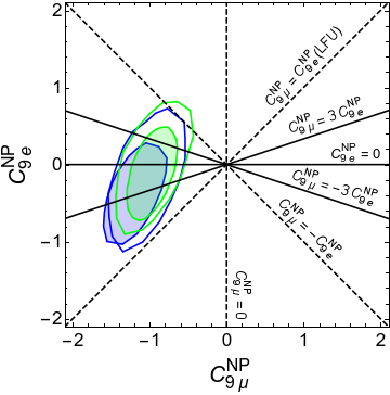
Although the involvement of NP in the muon sector is necessary to explain the anomalies, it is quite possible that NP affects the electron sector also. Recent global fits that take this into account mahmoudi-2021 ; matias-2021 indicate that the scenario with NP affecting can also explain the neutral-current flavor anomalies and other measurements reasonably well. These fits are shown in figure 1. The best-fit solution necessitates a negative value for in order to achieve a destructive interference with SM, since WC-SM . As can be seen from the figure, the fits do not determine the sign of , however they indicate .
In an earlier paper prev-paper , we had identified a class of minimal models that explain the flavor anomalies through the NP contributions to and , in a bottom-up approach. These models augmented SM by a symmetry, which was instrumental in generating the LFUV needed, and was broken spontaneously at the low scale by an SM-singlet scalar . Three right-handed neutrinos helped generate neutrino masses through the Type-I seesaw mechanism, with the same scalar instrumental in obtaining the appropriate texture zeros that give rise to the observed neutrino mixing pattern. The number of particles beyond the SM was minimal – apart from the gauge boson associated with the , one only needed the scalar and an additional Higgs doublet to generate quark mixing. Appropriate -charges were given to all particles such that the models are anomaly-free, fermions charges are vector-like, and experimental constraints from flavor physics — in particular the negative sign of needed for explaining the anomaly — were satisfied. This class of models was consistent with all the experimental measurements available at that time rk-2014 ; utfit ; atlas-dilepton-old . Indeed, even with the current data, the specific one-dimensional scenario in ref. prev-paper predicting is quite close to the best fit, while that with also provides a very good fit matias-2021 , as can also be seen from figure 1. Such scenarios correspond to the leptonic symmetry combinations , with unconstrained .
In this article, we show that recent strong constraints on the mass and coupling of the boson from collider experiments atlas-dilepton ; cms-dilepton make the above models unviable, if they are minimal flavor violation (MFV)-like, i.e. if the mixing parameters involved in the and sector are CKM-like. However, if this requirement, imposed implicitly on the class of models in prev-paper , is relaxed by a single parameter, a broader class of non-MFV models emerges, which retains all the desirable properties of the above models. Among them the scenarios with non-zero NP contributions to survive the strong collider constraints, while the scenarios with only NP contributions to stay disallowed. This new class of non-MFV models thus offers the most preferred candidates for the solutions of the neutral-current flavor anomalies through a symmetry. We term these as “frugal” models, since the number of particles beyond SM needed to complete these models are minimal. Note that the number of additional particles in this model stays the same as that in ref. prev-paper .
Several papers Buras:2013qja ; Altmannshofer:2014cfa ; Crivellin:2015mga ; Celis:2015ara ; prev-paper ; Bonilla:2017lsq ; Tang:2017gkz ; Bian:2017xzg ; Fuyuto:2017sys ; King:2018fcg ; Duan:2018akc ; Allanach:2018lvl ; Allanach:2019iiy ; Altmannshofer:2019xda ; less-MFV-crivillin ; Baek:2020ovw ; ben-b3-lmu ; Davighi:2021oel ; Bause:2021prv have focused on models as the solutions to the anomalies, either in isolation or by combining them with some other well-motivated SM problems, like neutrino masses, dark matter, fermion mass heirarchy, etc. With the current stringent colliders constraints Greljo:2017vvb ; atlas-dilepton ; cms-dilepton ; Allanach:2019mfl , the models have increasingly focused their attention on the scenarios where the collider constraints can be minimized. Examples of these include the models with only third generation of quarks charged under the new gauge symmetry Allanach:2018lvl ; Allanach:2019iiy ; ben-b3-lmu ; Bonilla:2017lsq , and models with vector-like additional quarks charged under the new symmetry Altmannshofer:2014cfa ; Bonilla:2017lsq . Some of the recent works have combined symmetry and leptoquarks for simultaneously explaning anomalies and the muon discrepancy Greljo:2021npi . In this manuscript, we follow the principle of frugality in adding new particles to the SM, and identify a class of symmetries which can simultaneosuly explain the anomalies and neutrino mixing.
The paper is organized as follows. In section 2, we recap the bottom-up construction of the class of models that address the anomalies, quark mixing, and neutrino mixing pattern. In particular, we describe the algorithm for assigning appropriate -charges to particles, while obeying the theoretical and experimental constraints. In section 3, we discuss the constraints on the mass and coupling of boson in these models from neutral meson mixing and collider data. In section 4.1, we show that the after incorporating the experimental constraints, the “MFV-like” models do not survive. section 4.2 shows that the introduction of a single non-MFV parameter allows a larger class of models to account for the flavor anomalies, while being consistent with all available constraints. Section 5 summarizes our results, and concludes.
2 Constructing models in a bottom-up approach
In this section, we recap our bottom-up approach prev-paper to identify models with a vector-like symmetry that can explain the anomalies through the NP WCs and . We denote the generic form of this symmetry as
| (2) |
where denotes the generation baryon number and denotes the lepton number for j-type lepton. The corresponding -charges of fermions are listed in Table 1. Note that in addition to the SM fermions, we also have three right-handed neutrinos.
| Fields | ||||||
The gauge symmetry of the SM forces the -charges of particles belonging to the same doublet to be identical. The fermion -charges are vector-like, which helps in anomaly cancellation, and also ensures that the contribution from the NP axial-vector currents vanishes, i.e. . The anomaly cancellation in this case is simple and further leads to only one condition
| (3) |
Before analyzing the detailed quantitative constraints on the parameters, desirable conditions on these parameters may be obtained using the following considerations:
-
•
The NP should not significantly affect the observables in neutral meson mixing, which have been found to match the SM predictions to a great precision.
-
•
The mass matrices of up-type and down-type quarks should be able to give rise to the appropriate Cabibbo-Kobayashi-Maskawa (CKM) matrix.
-
•
There should not be any massless goldstone bosons produced due to symmetry breaking.
-
•
The Type-I seesaw mechanism should yield the observed pattern of neutrino masses and mixing.
-
•
As indicated by global fits to the flavor anomaly data, the magnitude of NP coupling of electron should be smaller than that of muon.
-
•
The NP contribution must have a negative sign.
We shall apply these conditions successively in the following subsections.
2.1 -charges of quarks and the CKM matrix
The origin of the CKM matrix is in the diagonalization of up-type quark mass matrix and the down-type quark matrix by the bi-unitary transformations
| (4) |
The CKM matrix is then given by .
In the presence of a new gauge symmetry, the flavor-changing neutral currents (FCNC) induced by the new gauge boson would affect the neutral meson mixings by giving additional tree-level contributions to the box diagram in the SM. We focus on the constraints from CP violation in mixing (), and the mass splitting as well CP-violation in as well as mixing. We ignore constraints from , since its value is dominated by long distance effects Grinstein:2015nya . We also do not incorporate constraints from mixing for the same reason. The NP contribution may be calculated by writing down the Lagrangian for left-handed d-type quarks in their mass basis:
| (5) |
where . As shown in ref. prev-paper , the mixing in the right-handed d-quark sector may be chosen to be small, so that the contributions due to right-handed currents stay subdominant. The relevant matrix elements that control the dominant NP contributions in the , and systems may be written as
| (6) | |||||
| (7) | |||||
| (8) |
where the unitarity of has been used. The choice , and the small values of and , allow us to minimize the strong constraints from the sector and somewhat weaker constraints from the and sectors. The condition also implies an underlying flavor symmetry present in the Lagrangian, which is broken only by the Yukawa interactions isidori-straub . This has also been referred to as “less-minimal flavor violation” less-MFV ; less-MFV-crivillin . The additional choice (or equivalently, ) made in ref. prev-paper makes the scenario “MFV-like”, wherein the combinations of CKM elements contributing to the mixing in the and sectors are the same as those in the SM. It also ensures that the NP contribution from the second term to mixing is suppressed by , where is the Cabibbo angle.
We continue to use the condition in this paper. Later, for non-minimal scenarios, we will relax the condition , however the smallness of will still be valid, keeping in mind the stringent constraints from kaon oscillation data.
The condition (i.e. ) also impacts the structure of the Yukawa matrices. Since in our framework, the SM Higgs doublet is uncharged under , the only nonzero elements in the SM Yukawa matrix can be the three diagonal elements and the off-diagonal elements in the first two generations. This would force the - and - mixings in the CKM matrix to be zero. In order to prevent this, the SM needs to be augmented with an additional doublet whose -charge equals , or equivalently, . This would result in the NP contribution to the Yukawa matrices of up-type and down-type quarks in the form
| (9) |
where denotes nonzero elements. These off-diagonal elements give rise to the required mixing in the 2-3 and 1-3 sector, to reproduce the CKM matrix prev-paper . These Yukawa matrices can now give rise to the mass matrices
| (10) |
where and are the vacuum expectation values of the SM Higgs and the NP Higgs , respectively. The matrices and are diagonalized by the unitary matrices , , and , as shown in eq. (4). Note that the requirement of is instrumental in generating the CKM matrix with only one additional Higgs doublet.
2.2 -charges of scalars
Among the two Higgs doublets and , the former is a singlet under , to ensure nonzero diagonal elements in the flavor basis. The latter has an -charge equal to , as seen above.
The absence of a massless pseudoscalar, which would be created due to the breaking of a global symmetry in the Lagrangian, necessitates the introduction of an extra scalar , which has the same -charge as prev-paper . It allows a term in the scalar sector, which yields a mass for the pseudoscalar after the breaking of where gets a vacuum expectation value. The -charge of also needs to be .
2.3 -charges of leptons and Neutrino mixing
The global fits to neutral-current flavor anomalies and other data in the plane strongly indicate , which indicate as seen in figure 1. We therefore take this to be one of the conditions on our model. The value of remains unconstrained from the current measurements.
We determine the -charges of the leptons which can explain the patterns of neutrino mixing well. In particular, we desire that the leptonic mixing arises completely in the neutrino sector, where the neutrino mass is generated by the Type-I seesaw mechanism. However, since the -charges of the three lepton generations are, in general, different, it would not be possible to generate off-diagonal elements in the neutrino mass matrix, which are needed for the large neutrino mixing observed. In our model, this can be achieved without the need for any additional particle, but by using the interactions of the neutrinos with the scalar that is already present prev-paper . The terms contributing to neutrino mass are:
| (11) |
where is the Dirac matrix, is the Majorana mass matrix of right-handed neutrinos, and are flavor indices. The effective Marorana mass matrix after the symmetry breaking becomes
| (12) |
where is the vacuum expectation value of . Thus the mass matrix gets off-diagonal elements, which further lead to the mixing of left-handed neutrinos, through Type-I seesaw formula
| (13) |
In order for the above neutrino mass matrix to reproduce the observed neutrino mixing pattern, only certain texture-zero patterns of are allowed Grimus:2004hf ; neutrino-textures . A subset of these patterns may be created by appropriate choices of the values of , and prev-paper . A further subset satisfies the requirement . The leptonic symmetries that satisfy all these criteria are:
-
•
or , with ,
-
•
or , with .
Here is the overall multiplicative factor.
2.4 Scenarios indicated by the bottom-up construction
Inferring the -charges of leptons from the allowed leptonic symmetries, and using the conditions and , the -charges of all the other particles are fixed automatically by demanding the theory to be anomaly free. The -charges of all leptons, in turn, are fixed up to an overall multiplying factor as seen in the last section. We fix the normalization by choosing so as to make . All the scenarios thus determined are listed in Table 2. We further categorize them depending on their values of and . This ensures that flavor constraints for scenarios belonging to the same category are identical. Note that the categories A, B and C listed in table 2, with negative values, are the same as given in prev-paper . The category D from ref. prev-paper is not present in the current version because of the imposition of . In addition, have also included the categories AA, BB and CC with positive values. This inclusion completes the set of scenarios allowed by conditions in sections 2.1, 2.2, 2.3. Note that for the categories in each pair (A, AA), (B, BB), and (C, CC), the leptonic symmetries are identical, but the sign of is different.
| Category | Scenario | Leptonic symmetry | |||||||
| A | A1 | -1 | |||||||
| A2 | -1 | ||||||||
| B | B1 | ||||||||
| B2 | |||||||||
| C | C1 | ||||||||
| AA | AA1 | 1 | |||||||
| AA2 | 1 | ||||||||
| BB | BB1 | ||||||||
| BB2 | |||||||||
| CC | CC1 |
2.5 The sign of and the sign of
The NP in our class of models influences primarily through the Wilson coefficients . The contributions to are small due to the small mixing angles in (see ref. prev-paper and section 4.2). The tree-level contributions to operators are zero. They may arise due the mixing, and vanish in the small mixing limit. The effective Hamiltonian relevant for the process is
| (14) | |||||
Since , the above equation is equivalent to
| (15) |
Note that the WCs have scale dependence, however the qualitative inferences in this section do not change while running from the scale to . From eq. (15), the two relevant Wilson coefficients are related by .
From the global fits, we have seen that the sign of needed to explain the observed anomalies has to be negative, for the NP to destructively interfere with the SM, where is positive WC-SM . This leads to
| (16) |
i.e., either the charge is negative, or the ratio
| (17) |
is negative. In ref. prev-paper , the assumption of led to , so that was always unity. As a result, only those symmetry combinations where had been selected. These are the categories A, B, C shown in Table 2. In this paper, we follow a generalized approach, without the assumption . This allows three additional categories, viz. AA, BB and CC, as shown in Table. 2, where the sign of is positive.
3 Experimental constraints
We work in the limit where all additional NP particles apart from are decoupled, and determine constraints in the plane of . The global fits already provide constraints on these parameters from radiative, semileptonic, and leptonic B decays. These parameters can be further constrained by collider searches and the neutral meson mixing data, which we describe in the following subsections. The constraints from neutrino trident production are sub-leading for the relevant mass-coupling range of ben-b3-lmu , and electroweak precision constraints can be evaded when mixing is taken to be small Erler:2009jh and the other NP particles are decoupled; these constraints are not included in our analysis.
3.1 Collider constraints
The large amount of data being collected at the LHC strongly constrains any new physics that couples to light quarks. Our scenarios in table 2 necessarily have non-zero couplings of to the first two generations of quarks. Therefore, the particle will be produced at the LHC for low and high enough values. Furthermore, even a that couples dominantly to the third generations may be produced in a pp collision, albeit with a smaller cross section due to the smaller parton fraction in the proton. The non-observation of any such particle so far puts severe constraints on model parameters. The main observations that would constrain our class of models are:
-
•
Top-quark pair production limits from CMS:2020tvq ; ATLAS:2020aln ; ATLAS:2020lks
-
•
Dijet limits from , including ATLAS:2019fgd
-
•
Dilepton limit from atlas-dilepton ; cms-dilepton (including the non-resonant shape of the distribution tail altas-non-resonant ; cms-non-resonant )
As we show below, the most stringent limits come from dimuon searches. A comparison of the limits from all above observables can be seen in figure 2.
For searches, currently there is a measurement of pair production cross section with 35.9 fb-1 data from CMS CMS:2020tvq and 139 fb-1 data from ATLAS ATLAS:2020aln . Limits can be calculated either by using the total cross section or the invariant mass spectrum shape in addition. The best measurement for the total cross section is currently pb ATLAS:2020aln , and is completely consistent with the calculated SM cross section. We therefore require that the contribution from NP to the total cross section keeps the prediction less than two sigma away from the measured value. Further incorporating the spectral shape, a lower bound TeV is obtained for , as can be seen in figure 2.
For TeV, the background for dijet searches is high as compared to that for the searches, and hence the sensitivity of searches is better. However, at higher masses, the dijet searches give slightly stronger constraints. For example, TeV for , as seen in figure 2.
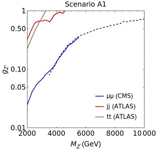
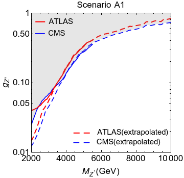
Our condition implies that the constraints from the di-electron searches would always be weaker than those from the dimuon searches. Hence, we focus on the dimuon channel. Experiments provide measurements of the invariant mass spectrum in the dimuon final state. Due to the simplicity of the final state, this may be interpreted in terms of a 95% upper limit on the production cross-section of (with minimal fiducial cuts). The parameter space () can then be constrained in any given scenario by comparing the theoretical production cross-section with the experimental 95% confidence limits. Such upper limits are available from the ATLAS experiment atlas-dilepton for TeV, and from the CMS experiment cms-dilepton for TeV. We use the constraints from CMS, which are slightly stronger than those from ATLAS, to represent the dimuon limits. As we see from figure 2, dimuon constraints are much stronger than either or dijet constraints for the scenario A1 (or equivalently, AA1). This observation remain true for all scenarios listed in table 2.
Using the number of observed events with high invariant mass, we can extend the dimuon limits to higher values of for which the calculated limits have not been published by the experimental analyses (see figure 2). The details of our calculations are explained in appendix A. The published bounds from CMS are available for TeV. Our calculated limits agree with these limits in the region TeV, thereby justifying the method used for extrapolation. For the rest of this study, we use the published CMS dimuon limits upto TeV, and our extrapolation for masses TeV.
Note that a 10 TeV can be excluded for high-enough coupling for all of our scenarios. On the other hand, requiring at least three events as a threshold for detection puts the LHC reach for the discovery of to TeV, depending on the scenario in table 2.
3.2 Neutral meson mixing constraints
Apart from mediating tree-level transitions, the additional particle would also be responsible for generating tree-level mixing in , and sectors. These new physics contributions are heavily constrained from data utfit . Since the mixing constraints are not taken into consideration in global fits matias-2019 ; mahmoudi-2019 ; matias-2021 ; mahmoudi-2021 , one has to incorporate them separately. Additionally, the new physics contributions generated by only affect the operators with left handed quark currents, as the right handed mixing is smaller in comparison to the left handed mixing (see ref. prev-paper and section 4.2). Hence contributes to the same operators as in the SM. We get
| (18) |
where at the scale are given as
| (19) |
Here generically refers to one of the , or meson. Note that while the CKM factors explicitly appear for mixings, they are conventionally absorbed in . After incorporating the running of the effective operators at one-loop order in QCD at scale buras-review , the WCs are obtained as
| (20) |
where stands for , or . Note that the running of SM and NP is identical after the scale, hence we have taken the running here only upto -mass scale. These additional contributions to mixing get constrained from the measurements. The constraints on and CP-violating phases are parameterized utfit in terms of
| (21) |
which can be studied in the plane of for a given symmetry and a given . Note that as mentioned in section 2, we do not consider the constraint from as it is dominated by long distance corrections utfit . For constraining our model parameter, we shall require that the allowed parameter space lies within 2 uncertainties for all these five observables, viz. , , , , and .
4 Testing the scenarios against experimental constraints
In any given scenario, the flavor constraints crucially depend on . Indeed, as can be seen in eq. (15), the value of is related to through , which depends on . In ref. prev-paper , we had chosen the MFV-like scenario and , which gave rise to for and mixing. In this paper, we will also allow more general scenarios for .
4.1 “MFV-like” scenarios with
When , the CKM factors in eq. (15) cancel, and the Wilson coefficient simplifies to
| (22) |
The desired negative value of is obtained if . This points towards the scenarios belonging to the categories A, B and C listed in table 2.
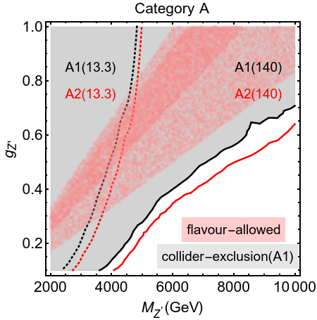
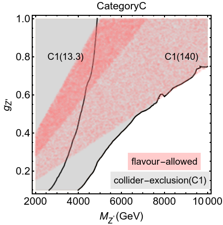
We now subject these scenarios to the experimental constraints discussed in section 3. The results are presented in fig 3. Note that for scenarios belonging to the same category, the global-fit constraints are identical, and so are the neutral meson mixings constraints. However collider constraints are different for sub-scenarios (like A1 and A2) which have different -charge assignments for quarks. We can clearly see that, on one hand, the allowed bands from global-fit have started to become narrower, while on the other hand, the constraints from LHC are becoming considerably more stringent. The current data with 140 fb-1 total integrated luminosity cms-dilepton has essentially ruled out all the parameter space for these MFV-like models.
The freedom of choice of allows us to find scenarios that survive the stringent collider and meson-mixing constraints above. This will be shown in the next subsection.
4.2 Non-minimal flavor violating (non-MFV) scenarios
Transition from MFV-like mixing, i.e. , to non-MFV mixing with would be severely constrained by measurements in the sector, where the value of as given in eq. (21) is very well measured. However, these constraints can be evaded if is chosen to be real. In the rest of the paper, we shall continue with real .
As seen in section 2.5, the resolution of anomalies needs . Writing the real in terms of three mixing angles , , (similar to the CKM parameterization), in eq. (17) can be written as
| (23) | |||||
Note that, since can have either sign, the sign of can now be positive as well as negative. This allows the categories AA, BB and CC from table 2 to be viable candidates, in addition to the categories A, B and C considered earlier. Moreover, if the magnitude of is large, the required values of may become possible even with lower values of , as can be seen from eq. (15). However, the parameter cannot be too large, otherwise the simultaneous explanation of anomalies along with neutral meson mixing constraints from mixing would be difficult. Thus, a modest enhancement of is required to make these scenarios compatible with the global fits, neutral meson mixing data, and collider constraints.
Since , one would need for the enhancement in . In a simplified scenario, we can take and , which leads to
| (24) |
The choice of small and would also limit the severity of collider constraints. Note that our choice of is the same as that in ref. ben-b3-lmu . This choice of makes the constraints from mixing to be very crucial. From eq. (4), one can then obtain the corresponding matrix in as
| (25) |
It can be seen from this equation, that the mixing induced due to remains small unless we are close the limit where . We will stay away from these limits in this paper. Our approximation of ignoring the right handed currents, used in eqns. (5, 14) and section 3.2, is thus justified.
The introduction of non-minimal flavor violation in its frugal form has allowed us an extra parameter . The sign of dictates that the symmetries in categories A, B and C will work if is in the first quadrant, and categories AA, BB and CC will work if lies in the second quadrant.
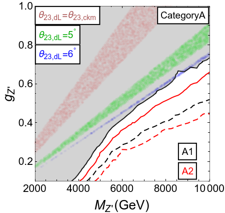
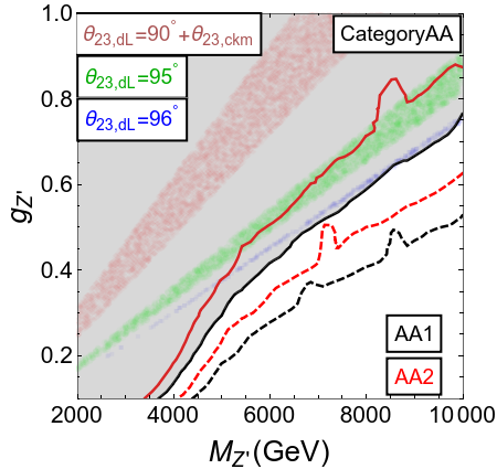
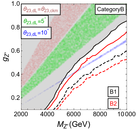
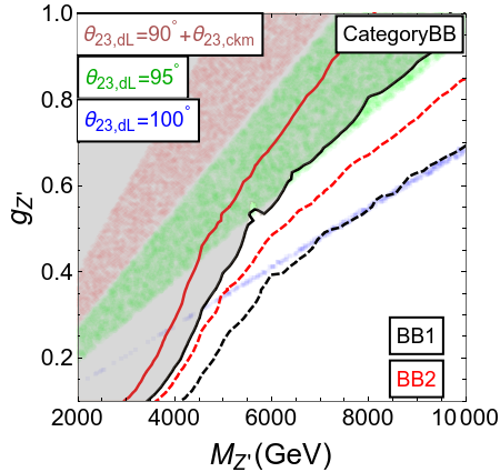
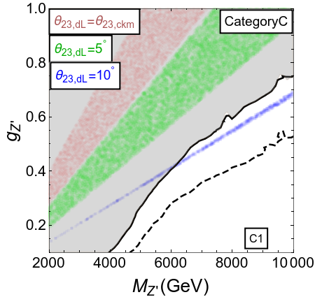
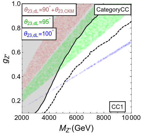
In figure 4, we present the main results of this section in the plane of , for a few selected values of . From the figure, the following observations may be made:
-
•
For a given category, the combined constraints from the global fit and neutral meson mixing with a given value are identical to those with .
-
•
As the flavor constraints depend on , they can be identical for the scenarios that have the same value of but opposite sign, with values differing by . For example, compare A() with AA(). The collider constraints for these pairs are, however, different.
-
•
The constraints for B2 and C1 are almost identical, and so are the constraints for BB2 and CC1. This is because the scenarios in these pairs carry identical charges for quarks and muons. They differ only in the sign of , however the global fit mahmoudi-2021 is nearly symmetric in , as can be seen in figure 1.
-
•
In the categories A, B, C, smaller values satisfy the flavor constraints, neutrino mixing, and collider constraints simultaneously. However, this is not possible for larger values, as may be seen from the thinning of the colored bands with an increase in . This happens because is proportional to , while the mixing is sensitive to , and does not allow it to take a larger value. A similar comment applies to the categories AA, BB, CC, where the allowed values are .
-
•
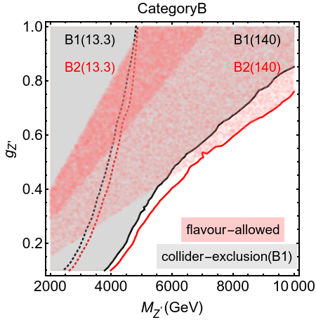
The symmetries belonging to categories A and AA, where new physics contributes only in the muon (and/or) tau sector, stay ruled out from the current constraints on the dimuon resonance search at LHC cms-dilepton . At higher luminosities of 3000 fb-1 at the LHC, the parameter space relevant for scenarios B1, B2, C1 and BB1 may also be completely probed by the collider searches, for TeV.
-
•
The scenarios BB2 and CC1 will be the most difficult to rule out even with the high luminosity run of the LHC. This is expected since they have the smallest -charges for quarks among all the categories (see table 2). These scenarios correspond to the leptonic symmetry combinations , with positive values.
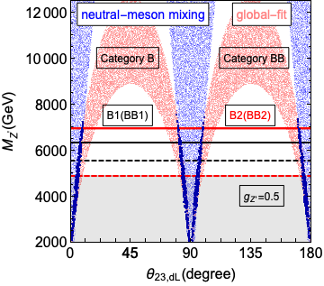
In figure 5, we show the incompatibility of the constraints with the global fit at large values, for categories B and BB as representative examples. All our findings from figure 4 may be reconfirmed here. The neutral-meson mixing constraints for the pairs of categories (B, BB) are identical and the global fit constraints are mirror images of one another around . Only the tiny narrow regions, shaded in purple, survive both these simultaneously. It can also be noted that the collider constraint is the weakest for the scenario BB2. Hence, this scenario is expected to be the most difficult to rule out even with the higher luminosity runs of LHC.
Indeed, for the scenarios with first two generations of quarks charged under , it is difficult to simultaneously explain the anomalies along with neutrino mixing and neutral meson mixing, while staying compatible with the collider constraints. In this section, we identified a suitable simple choice of that can circumvent the otherwise stringent collider constraints for some of the scenarios, without the addition of any new particle in our construction. Even with this non-minimal flavor violation, the scenarios with leptonic symmetry combinations and stay ruled out. The leptonic symmetry combinations and emerge as the viable ones with the current data, though they will be further probed with the high-luminosity data at the LHC, with 3000 fb-1 of integrated luminosity. Thus in our frugal setup, the data seems to hint towards the possibility of new physics in the electron as well as tau sector, in addition to the muon sector.
5 Summary and concluding remarks
In our present work, we identify a class of models which can simultaneously explain the anomalies and neutrino mixing patterns. We identify the -charges using hints from the previous measurements and global fits in a bottom-up approach. We follow the principle of frugality, i.e., try to minimize the number of additional fields beyond SM. The only fields added are three right-handed neutrinos, an additional SM doublet Higgs, and a SM-singlet scalar. The methodology followed here is similar to the one considered in ref. prev-paper .
We focus on the construction of scenarios where the NP contributes primarily to as well as . The global fits matias-2021 ; mahmoudi-2021 imply the sign of has to be necessarily negative, and the magnitude of new physics contributions in electron has to be smaller than muon. The sign of is not constrained by the global fits. The choice of vector-like -charges ensures vanishing , and helps make the theory anomaly-free. Note that contributions due to also remain negligible in our analysis.
The stringent constraint from implies equal charges for the first two quark generations. The requirement of generating interaction through tree-level exchange of dictates that the -charge of the third generation quarks must be necessarily different from the first two. The additional Higgs doublet with an appropriate -charge then generates the desired quark mixing.
The singlet scalar breaks the symmetry spontaneously and helps generate the neutrino masses and their mixing pattern. The choice of equal -charges of and prevents the emergence of a massless Goldstone boson in the spectrum. This also relates the -charges of quarks with the leptons, which can be uniquely determined using the requirement of anomaly cancellation.
The observed neutrino mixing patterns restrict the possible leptonic symmetries in our frugal set-up, where the scalar singlet is sufficient to generate the neutrino masses and mixing patterns. This also leads to an important consequence that all the identified scenarios necessarily have non-zero -charges for all generations of quarks. This may be contrasted with the scenarios where only third generation of quarks are charged, e.g. symmetry. Such scenarios would require more particles than those that are already present in our frugal set-up, for simultaneous explanations of neutrino mixing patterns and flavor anomalies.
To generate the correct (negative) sign of , we find that the combination should be negative. In ref. prev-paper , where the MFV-like mixing was chosen, we had , which implied that only the scenarios with can explain the flavor anomalies well. However, allowing the departure of from enables us to select a broader set of scenarios with both positive and negative signs of . In our analysis, we work in the limit where all additional NP particles apart from are decoupled, so that the relevant parameter space is that of the mass and coupling of , viz. () for different choices of .
Experimental limits from the collider searches and neutral meson mixing give the dominant constraints on (). The neutral meson mixing constraints are evaluated for and oscillations. We compare the exclusion limits from resonance searches in dijet, and dilepton channels, and find that the CMS dimuon search gives the most stringent constraints for all scenarios. We find that, after taking into account the recent full run-2 data from the LHC, no MFV-like scenario compatible with the flavor anomalies remains allowed. The stringent collider constraints arise because of the non-zero -charge assignment of the first two quark generations, necessitated in our frugal set-up.
By relaxing the assumption of the CKM-like mixing for , the collider constraints can be made compatible with the flavor anomalies for scenarios with leptonic symmetries of the form and . We demonstrate this with a simple non-MFV scenario where only involves mixing between the second and the third generations, parameterized by . In order to generate the desired sign of , the new mixing angle necessarily lies in the first (second) quadrant for scenarios with negative (positive) . Note that scenarios with NP contributions present only in muon (and/or tau), stay ruled out even when the mixing is allowed to be non-MFV.
We extrapolate the resonant dimuon search limits to values upto 10 TeV, to investigate future prospects for a discovery. While the scenarios with leptonic symmetry and negative , as well as with either sign of , will be completely probed with 3000 fb-1 total integrated luminosity, the scenarios with and positive will be difficult to rule out even with the high luminosity run at the LHC.
To conclude, our class of frugal models, that employ a minimal number of particles beyond the SM, can account for anomalies as well as the neutrino mixing pattern. The recent stringent collider constraints can be overcome by a one-parameter choice of , without any additional particles, for a set of scenarios where couples to all three lepton generations.
Acknowledgments
The authors would like to thank Abhaya Kumar Swain and IACS for help with computational resources. A.D. acknowledges support of the Department of Atomic Energy (DAE), Government of India, under Project Identification No. RTI4002. ND acknowledges support from the Department of Science and Technology through grant number SB/S2/RJN-070.
Appendix A Extrapolation of exclusion limits from dimuon searches
Here we describe the procedure for extrapolating the exclusion limits from collider searches, using the ATLAS dimuon search atlas-dilepton as an example. In general, experiments provide the observed invariant mass spectrum in each final state. This final shape depends on the production cross section, branching fraction for the relevant decay mode, as well as the detector acceptances and efficiencies. For a more complicated observable, it would be difficult for a phenomenological study to use this information without detailed description of the efficiencies. However, in the dimuon case, once the basic fiducial cuts (described in ref. atlas-dilepton ) are taken into account, we find that we can reproduce the published experimental limits accurately.
The total number of events expected from a signal hypothesis (choice of charges, , and ) can be obtained by
| (26) |
where is the production cross section into the dimuon final state, is the efficiency of the fiducial cuts, and is the integrated luminosity.
A simple Poisson likelihood can be constructed using binned data. In our case, since we are only interested in the extrapolation to high masses, we simplify the problem by looking at only the last bin, which collects all observations with the dilepton invariant mass TeV for the ATLAS dilepton search atlas-dilepton . For a single bin, Poisson likelihood () for observed number of events and expected number of events is given as
| (27) |
leading to
| (28) |
Here and are the expected number of signal and background events, respectively. In order to get 95% confidence limits, the above equation is solved for for , which corresponds to one-sided p-value of 0.05 for one degree of freedom.
The choice of only one bin for the high mass tail of the resonance mass distribution implies that our upper limits are conservative, since we do not use the information on the modification of the shape of the distribution due to non-resonant contribution. Figure 6 shows that this prescription matches the high-end ( TeV) official limits very well, and therefore can be used reliably. This simple formulation thus allows us to extrapolate the limits for up to 10 TeV, as well as to calculate expected sensitivities from future runs at the LHC (assuming that all events scale with integrated luminosity).
A similar exercise may be carried out with the CMS data as well. However, we find that a flat overall efficiency factor of 0.4 is needed to reliably get the same upper limits as published by CMS cms-dilepton where the last bin collects all events with dimuon invariant mass greater than TeV. The comparison of our calculation with published ATLAS and CMS are shown in figure 6. Even though our calculated CMS limits deviate from the ones published with full shape analysis for low as expected, they match very well for all values of TeV, and can be used for extrapolation to high masses with confidence.
References
- (1) ATLAS, CMS, LHCb Collaboration, E. Graverini, Flavour anomalies: a review, J. Phys. Conf. Ser. 1137 (2019) [arXiv:1807.11373].
- (2) G. Hiller and M. Schmaltz, Diagnosing lepton-nonuniversality in , JHEP 02 (2015) [arXiv:1411.4773].
- (3) M. Bordone, G. Isidori, and A. Pattori, On the Standard Model predictions for and , Eur. Phys. J. C 76 (2016) [arXiv:1605.07633].
- (4) LHCb Collaboration, R. Aaij et al., Test of lepton universality in beauty-quark decays, arXiv:2103.11769.
- (5) LHCb Collaboration, R. Aaij et al., Test of lepton universality using decays, Phys. Rev. Lett. 113 (2014) [arXiv:1406.6482].
- (6) LHCb Collaboration, R. Aaij et al., Search for lepton-universality violation in decays, Phys. Rev. Lett. 122 (2019) [arXiv:1903.09252].
- (7) Belle Collaboration, A. Abdesselam et al., Test of Lepton-Flavor Universality in Decays at Belle, Phys. Rev. Lett. 126 (2021) [arXiv:1904.02440].
- (8) LHCb Collaboration, R. Aaij et al., Angular Analysis of the Decay, Phys. Rev. Lett. 126 (2021) [arXiv:2012.13241].
- (9) ATLAS Collaboration, M. Aaboud et al., Angular analysis of decays in collisions at TeV with the ATLAS detector, JHEP 10 (2018) [arXiv:1805.04000].
- (10) Belle Collaboration, A. Abdesselam et al., Angular analysis of , in LHC Ski 2016: A First Discussion of 13 TeV Results, 4, 2016. arXiv:1604.04042.
- (11) LHCb Collaboration, R. Aaij et al., Measurement of -Averaged Observables in the Decay, Phys. Rev. Lett. 125 (2020) [arXiv:2003.04831].
- (12) LHCb Collaboration, R. Aaij et al., Angular analysis and differential branching fraction of the decay , JHEP 09 (2015) [arXiv:1506.08777].
- (13) A. Khodjamirian, T. Mannel, A. A. Pivovarov, and Y. M. Wang, Charm-loop effect in and , JHEP 09 (2010) [arXiv:1006.4945].
- (14) S. Descotes-Genon, L. Hofer, J. Matias, and J. Virto, On the impact of power corrections in the prediction of observables, JHEP 12 (2014) [arXiv:1407.8526].
- (15) D. Lancierini, G. Isidori, P. Owen, and N. Serra, On the significance of new physics in decays, arXiv:2104.05631.
- (16) A. K. Alok, A. Dighe, S. Gangal, and D. Kumar, Continuing search for new physics in decays: two operators at a time, JHEP 06 (2019) [arXiv:1903.09617].
- (17) L.-S. Geng, B. Grinstein, S. Jäger, S.-Y. Li, J. Martin Camalich, and R.-X. Shi, Implications of new evidence for lepton-universality violation in decays, arXiv:2103.12738.
- (18) W. Altmannshofer and P. Stangl, New Physics in Rare B Decays after Moriond 2021, arXiv:2103.13370.
- (19) M. Algueró, B. Capdevila, S. Descotes-Genon, J. Matias, and M. Novoa-Brunet, global fits after Moriond 2021 results, in 55th Rencontres de Moriond on Electroweak Interactions and Unified Theories, 4, 2021. arXiv:2104.08921.
- (20) T. Hurth, F. Mahmoudi, D. M. Santos, and S. Neshatpour, More Indications for Lepton Nonuniversality in , arXiv:2104.10058.
- (21) M. Algueró, B. Capdevila, A. Crivellin, S. Descotes-Genon, P. Masjuan, J. Matias, M. Novoa Brunet, and J. Virto, Emerging patterns of New Physics with and without Lepton Flavour Universal contributions, Eur. Phys. J. C 79 (2019) [arXiv:1903.09578]. [Addendum: Eur.Phys.J.C 80, 511 (2020)].
- (22) A. Arbey, T. Hurth, F. Mahmoudi, D. M. Santos, and S. Neshatpour, Update on the b→s anomalies, Phys. Rev. D 100 (2019) [arXiv:1904.08399].
- (23) J. Albrecht, F. Bernlochner, M. Kenzie, S. Reichert, D. Straub, and A. Tully, Future prospects for exploring present day anomalies in flavour physics measurements with Belle II and LHCb, arXiv:1709.10308.
- (24) A. J. Buras, Weak Hamiltonian, CP violation and rare decays, in Les Houches Summer School in Theoretical Physics, Session 68: Probing the Standard Model of Particle Interactions, 6, 1998. hep-ph/9806471.
- (25) D. Bardhan, P. Byakti, and D. Ghosh, Role of Tensor operators in and , Phys. Lett. B 773 (2017) [arXiv:1705.09305].
- (26) G. Hiller and M. Schmaltz, and future physics beyond the standard model opportunities, Phys. Rev. D 90 (2014) [arXiv:1408.1627].
- (27) W. Altmannshofer, P. Ball, A. Bharucha, A. J. Buras, D. M. Straub, and M. Wick, Symmetries and Asymmetries of Decays in the Standard Model and Beyond, JHEP 01 (2009) [arXiv:0811.1214].
- (28) D. Bhatia, S. Chakraborty, and A. Dighe, Neutrino mixing and anomaly in U(1)X models: a bottom-up approach, JHEP 03 (2017) [arXiv:1701.05825].
- (29) UTfit Collaboration, C. Alpigiani et al., Summer 2018 new physics results, www.utfit.org/UTfit/ResultsSummer2018NP.
- (30) ATLAS Collaboration, Search for new high-mass resonances in the dilepton final state using proton-proton collisions at = 13 TeV with the ATLAS detector, ATLAS-CONF-2016-045.
- (31) ATLAS Collaboration, G. Aad et al., Search for high-mass dilepton resonances using 139 fb-1 of collision data collected at 13 TeV with the ATLAS detector, Phys. Lett. B 796 (2019) [arXiv:1903.06248].
- (32) CMS Collaboration, Search for a narrow resonance in high-mass dilepton final states in proton-proton collisions using 140 of data at , CMS-PAS-EXO-19-019.
- (33) A. J. Buras and J. Girrbach, Left-handed and FCNC quark couplings facing new data, JHEP 12 (2013) [arXiv:1309.2466].
- (34) W. Altmannshofer, S. Gori, M. Pospelov, and I. Yavin, Quark flavor transitions in models, Phys. Rev. D 89 (2014) [arXiv:1403.1269].
- (35) A. Crivellin, G. D’Ambrosio, and J. Heeck, Explaining , and in a two-Higgs-doublet model with gauged , Phys. Rev. Lett. 114 (2015) [arXiv:1501.00993].
- (36) A. Celis, J. Fuentes-Martin, M. Jung, and H. Serodio, Family nonuniversal Z’ models with protected flavor-changing interactions, Phys. Rev. D 92 (2015) [arXiv:1505.03079].
- (37) C. Bonilla, T. Modak, R. Srivastava, and J. W. F. Valle, gauge symmetry as a simple description of anomalies, Phys. Rev. D 98 (2018) [arXiv:1705.00915].
- (38) Y. Tang and Y.-L. Wu, Flavor non-universal gauge interactions and anomalies in B-meson decays, Chin. Phys. C 42 (2018) [arXiv:1705.05643]. [Erratum: Chin.Phys.C 44, 069101 (2020)].
- (39) L. Bian, H. M. Lee, and C. B. Park, -meson anomalies and Higgs physics in flavored model, Eur. Phys. J. C 78 (2018) [arXiv:1711.08930].
- (40) K. Fuyuto, H.-L. Li, and J.-H. Yu, Implications of hidden gauged model for anomalies, Phys. Rev. D 97 (2018) [arXiv:1712.06736].
- (41) S. F. King, and the origin of Yukawa couplings, JHEP 09 (2018) [arXiv:1806.06780].
- (42) G. H. Duan, X. Fan, M. Frank, C. Han, and J. M. Yang, A minimal extension of MSSM in light of the B decay anomaly, Phys. Lett. B 789 (2019) [arXiv:1808.04116].
- (43) B. C. Allanach and J. Davighi, Third family hypercharge model for and aspects of the fermion mass problem, JHEP 12 (2018) [arXiv:1809.01158].
- (44) B. C. Allanach and J. Davighi, Naturalising the third family hypercharge model for neutral current -anomalies, Eur. Phys. J. C 79 (2019) [arXiv:1905.10327].
- (45) W. Altmannshofer, J. Davighi, and M. Nardecchia, Gauging the accidental symmetries of the standard model, and implications for the flavor anomalies, Phys. Rev. D 101 (2020) [arXiv:1909.02021].
- (46) L. Calibbi, A. Crivellin, F. Kirk, C. A. Manzari, and L. Vernazza, models with less-minimal flavour violation, Phys. Rev. D 101 (2020) [arXiv:1910.00014].
- (47) S. Baek, A connection between flavour anomaly, neutrino mass, and axion, JHEP 10 (2020) [arXiv:2006.02050].
- (48) B. C. Allanach, explanation of the neutral current anomalies, Eur. Phys. J. C 81 (2021) [arXiv:2009.02197]. [Erratum: Eur.Phys.J.C 81, 321 (2021)].
- (49) J. Davighi, Anomalous bosons for anomalous decays, arXiv:2105.06918.
- (50) R. Bause, G. Hiller, T. Höhne, D. F. Litim, and T. Steudtner, B-Anomalies from flavorful U(1)’ extensions, safely, arXiv:2109.06201.
- (51) A. Greljo and D. Marzocca, High- dilepton tails and flavor physics, Eur. Phys. J. C 77 (2017) [arXiv:1704.09015].
- (52) B. C. Allanach, J. M. Butterworth, and T. Corbett, Collider constraints on Z′ models for neutral current B-anomalies, JHEP 08 (2019) [arXiv:1904.10954].
- (53) A. Greljo, Y. Soreq, P. Stangl, A. E. Thomsen, and J. Zupan, Muonic Force Behind Flavor Anomalies, arXiv:2107.07518.
- (54) B. Grinstein, TASI-2013 Lectures on Flavor Physics, in Theoretical Advanced Study Institute in Elementary Particle Physics: Particle Physics: The Higgs Boson and Beyond, 1, 2015. arXiv:1501.05283.
- (55) G. Isidori and D. M. Straub, Minimal Flavour Violation and Beyond, Eur. Phys. J. C 72 (2012) [arXiv:1202.0464].
- (56) R. Barbieri, D. Buttazzo, F. Sala, and D. M. Straub, Less Minimal Flavour Violation, JHEP 10 (2012) [arXiv:1206.1327].
- (57) W. Grimus, A. S. Joshipura, L. Lavoura, and M. Tanimoto, Symmetry realization of texture zeros, Eur. Phys. J. C 36 (2004) [hep-ph/0405016].
- (58) T. Araki, J. Heeck, and J. Kubo, Vanishing Minors in the Neutrino Mass Matrix from Abelian Gauge Symmetries, JHEP 07 (2012) [arXiv:1203.4951].
- (59) J. Erler, P. Langacker, S. Munir, and E. Rojas, Improved Constraints on Z-prime Bosons from Electroweak Precision Data, JHEP 08 (2009) 017, [arXiv:0906.2435].
- (60) CMS Collaboration, A. M. Sirunyan et al., Measurement of differential production cross sections using top quarks at large transverse momenta in collisions at 13 TeV, Phys. Rev. D 103 (2021) [arXiv:2008.07860].
- (61) ATLAS Collaboration, G. Aad et al., Measurement of the production cross-section in the lepton+jets channel at TeV with the ATLAS experiment, Phys. Lett. B 810 (2020) [arXiv:2006.13076].
- (62) ATLAS Collaboration, G. Aad et al., Search for resonances in fully hadronic final states in collisions at = 13 TeV with the ATLAS detector, JHEP 10 (2020) [arXiv:2005.05138].
- (63) ATLAS Collaboration, G. Aad et al., Search for new resonances in mass distributions of jet pairs using 139 fb-1 of collisions at TeV with the ATLAS detector, JHEP 03 (2020) [arXiv:1910.08447].
- (64) ATLAS Collaboration, G. Aad et al., Search for new non-resonant phenomena in high-mass dilepton final states with the ATLAS detector, JHEP 11 (2020) [arXiv:2006.12946]. [Erratum: JHEP 04, 142 (2021)].
- (65) CMS Collaboration, A. M. Sirunyan et al., Search for resonant and nonresonant new phenomena in high-mass dilepton final states at = 13 TeV, JHEP 07 (2021) [arXiv:2103.02708].
- (66) UTfit Collaboration, C. Alpigiani et al., Summer 2016 new physics results, www.utfit.org/UTfit/ResultsSummer2016NP.
- (67) T. Hurth, F. Mahmoudi, and S. Neshatpour, On the anomalies in the latest LHCb data, Nucl. Phys. B 909 (2016) [arXiv:1603.00865].