From the multi-terms urn model to the self-exciting negative binomial distribution
and
Hawkes processes

Anomalous diffusion is one of the most interesting topics in sociophysics and econophysics galam ; galam2 ; Man . Models describing these phenomena have correlations Bro ; W2 ; G ; M ; hod ; hui ; sch , and show several types of phase transitions. In our previous work, we investigated voting models for an information cascade Mori ; Hisakado2 ; Hisakado3 ; Hisakado35 ; Hisakado4 ; Hisakado5 ; Hisakado6 ; Mori6 . This model is a type of urn process that represents the correlations and has two types of phase transitions. One is the information cascade transition, which is one of the non-equilibrium phase transitions Hisakado3 . The other is the convergence transition of the super-normal diffusion that corresponds to an anomalous diffusion Hod ; Hisakado2 .

Financial engineering has led to the development of several products to hedge risks. These products protect against a subset of the total loss on a credit portfolio in exchange for payments, and provide valuable insights into the market implications of default dependencies and clustering of defaults M2010 ; M2008 ; Sch . This aspect is important, because the difficulties in managing credit events depend on these correlations. The Hawkes process was recently used to represent the clustering defaults of time series Haw ; kir ; qp ; err ; KZ ; KZ1 . The clustering defaults mean that as the number of events increases, the probability of the events increases. This phenomenon corresponds to self-excitation and constitutes a temporal correlation. From the physical view point this process is characterized by a phase transition from the steady state to the non-steady state. It is one kind of the non-equilibrium phase transitions and the relation between the Hawkes process and the branching process is shown in Haw2 . In fact the extinction phase of the branching process corresponds to the steady state in Hawkess process Hisakado8 . Confirmation of the steady state is important for finance and risk management to hedge risks because it is not possible to manage the non-steady state.

In our previous study, we discussed the parameter estimation of the urn process, which has a correlation in the same term, and considered a multi-year case with a temporal correlation Hisakado6 ; Mori6 . In this work, we introduce a new extended multi-term urn process and discuss the relationship between the new urn process and the Hawkes process. In the continuous time limit one can obtain the self-exciting NBD (SE-NBD) process and Hawkes process as the parameters approach certain limits.

We study the properties of the phase transitions of these processes. In fact the simultaneous and temporal effects of the correlation were confirmed by analyzing empirical default data. The results confirmed that the urn process fits more accurately than the Hawkes process. The reason is the variance of the intensity function is nonzero. In fact some firms effect many companies and some firms do not effect the companies. It is one of the effects of the network, because the network with hubs have the large variance of the degree distributions Hisakado7 .

The remainder of this article is organized as follows. In Section II, we introduce the multi-term urn process. We discuss the relationship between the Hawkes process and phase transition. In Section III we present our study of the phase transition of this model. In Section IV, we present the power law of the distribution function at the critical point. In Section V we discuss the application of the process to empirical data of historical defaults and confirm its parameters. Finally, the conclusions are presented in Section VI.

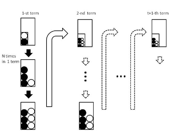
In this section, we consider a multi-term urn process that has correlations. In the first term, the urn contains $\theta_{0}$ red balls and $n_{0}-\theta_{0}$ white balls. Then, balls are sequentially taken out from the urn. For example, a single ball is taken out, after which we return the ball taken out to the urn and add $\omega$ balls of the same color to the urn. Thus, the total number of balls increases by $\omega$ a process, which is a correlation parameter in the same term, Hisakado . In fact as we take out more red balls, the probability that a red ball is taken out increases, because the number of red balls in urn increases. This is the correlation in the same term. We repeat the process $N$ times in the first term. Hence, the number of the total balls is $n_{0}+N\omega$ in the end of the first term. This is nothing but the Pólya urn model, which has a beta binomial distribution (BBD). We summarize the parameters for this urn model in Appendix A.

Next we extend the process to the multi-term process. We repeat the same process as the first process with the updated parameter $\theta_{t}$ at the $t+1$-th term. In the $t+1$-th term the urn contains $\theta_{t}=\theta_{0}+\sum^{t}_{i}k_{i}\hat{d}_{t-i+1}\tilde{\omega}$ red balls, and $n_{0}-\theta_{t}$ white balls. Here, the total number of initial balls is $n_{0}$, $\hat{d}_{i}$ denotes the kernel function or discount factor that represents the decrease of the effects of self excitation. Note that $\theta_{t}$ depends on the history of number of the taken out red balls. For the normalization we set $\hat{d}_{0}=1$. Here we introduce the variable $X_{i}$ which is the number of red balls taken out in the $i$-th term and its value is $X_{i}=k_{i}$. $\tilde{\omega}$ is one of the parameters for temporal correlation, where $\omega$ denotes the scale parameter for the added red balls. $\tilde{\omega}$ is the ratio of the number of balls placed back to the urn to the number of balls drawn from the urn, when $\hat{d}_{0}=1$ and $\hat{d}_{i}=0,i\geq 1$. In this case only the previous term affects the present term. In summary we update only the parameter $\theta_{t}$ and other parameters are fixed in each term.

As the first term we sequentially take out balls from the urn. After that we return the taken out ball to the urn and $\omega$ balls of the same color are added to the urn. We repeat the process $N$ times in this $t+1$-th term. It is the definition of the one term. After the process of $t+1$ term, we set the initial condition of $t+2$-term and continue the $t+2$-th process. Each term is also the Pólya urn model. In this model we use two kinds of correlations: the first is a correlation in the same term using the parameter $\omega$, and the other is the temporal correlation using the parameters $\tilde{\omega}$ which is independent from $\omega$ and $\hat{d}_{i}$, which is the kernel function. The temporal correlation decays as a function of time using the parameter $\hat{d}_{i}$.

In Hisakado6 , we introduced a similar urn process with a correlation in the same term and temporal correlation. The difference is the initial condition of the $t+1$-th term. The number of red balls is the same, but the number of white balls is $n_{0}-\theta_{0}+\sum_{i}^{t}(N-k_{i})\hat{d}_{t-i+1}\tilde{\omega}$, where $X_{i}=k_{i}$, and the total number of balls in the initial condition of each term is not constant, $n_{0}$.

When $k_{1}$ red balls are taken out in the 1-st term, $X_{1}=k_{1}$, the probability in the 1-st term can be calculated as

where $p=\theta_{0}/n_{0}$, $q=1-\theta_{0}/n_{0}$, and $\omega/n_{0}=\rho/(1-\rho)$. This is known as the beta binomial distribution $\mbox{BBD}(\alpha,\beta$,$N$) where $p=\alpha/(\alpha+\beta)$ and $q=\beta/(\alpha+\beta)$. Here, $\alpha$ and $\beta$ correspond to the parameters of the beta distribution in the continuous limit of BBD. Note that $\rho=1/(1+\alpha+\beta)$ plays the role of a correlation in this term Hisakado . In fact the variance of BBD is $Npq+N(N-1)pq\rho$ and the second term corresponds to the correlation in the same term. Hence, $\omega$ is the correlation parameter.

Herein we consider the temporal correlation by adjusting the initial conditions of the red balls, $\theta_{t}$ in each term. The temporal correlation is the decay of the correlation at different times, $\mbox{Cor}(X_{t},X_{t+\tau})$ as $\tau$ increases. The total number of balls in the initial condition of the each term is $n_{0}$. The expected value of the ratio of the taken out red balls in $t+1$-th term is $\theta_{t}/n_{0}$, where $\theta_{t}=\theta_{0}+\sum^{t}_{i}k_{i}\hat{d}_{t-i+1}\tilde{\omega}$. This implies that the events of the previous terms affect the present events. Here the number of the events is the number of the red balls taken out. As the number of the events increases, the expected value of the number of events in the next term increases. Hence, we can introduce the temporal correlation by adjusting the initial condition of each term. When $\theta_{t}=\theta_{0}$, there is no temporal correlation, because each term is independent.

Here we set the first double scaling limit $N/n_{0}=\Delta$, $N\rightarrow\infty$ and $n_{0}\rightarrow\infty$. We can obtain

where $M_{0}=\theta_{0}N/n_{0}=\theta_{0}\Delta$ and $K_{0}=\theta_{0}/\omega$. Here, $\sim$ means that the stochastic variable on the LHS obeys the probability distribution on RHS. This is a negative binomial distribution (NBD), $\mbox{NBD}(X_{1}=k_{1}|K_{0},M_{0}/K_{0})$. Parameter $M_{0}/K_{0}=\omega N/n_{0}=\omega\Delta$ is related to the correlation in this term. The mean and the variance of NBD is $M_{0}$ and $M_{0}+M_{0}^{2}/K_{0}$, respectively.

The negative binomial distribution $\mbox{NBD}(X_{1}=k_{1}|K_{0},M_{0}/K_{0})$ has another face:

where $\mbox{Poisson}(k_{1}|\lambda)$ is the Poisson process $\mbox{Gamma}(\lambda|K_{0},M_{0}/K_{0})$ is the gamma distribution. We show the proof Eq.(3) in Appendix B. From this result NBD is the Poisson process with the intensity function $\lambda$ which obeys the gamma distribution. In the multi-term model, we can decompose the process in the same way. Hence, $\lambda_{t}$ is the intensity function of the $t$-th term and obeying the gamma distribution. $\mbox{Gamma}(\lambda|K_{0},M_{0}/K_{0})$ has an average of $M_{0}$ and a variance of $M_{0}^{2}/K_{0}$. This means that the urn process in the 1-st term corresponds to the Poisson process with intensity function $\lambda$, which has a gamma distribution in the double scaling limit. The intensity function yields the variance of comparing the Poisson process, which has a constant intensity function. We refer to this as the NBD process.

Next, we define the $t+1$-th term with the temporal correlation Hisakado6 using the conditional probability. We define the conditional probability of $t+1$-th term,

where $k_{i}$ is the history of the number of red balls taken out. The conditional probability is defined by updating parameters $K_{t}$ and $M_{t}$. The only difference between the 1-st term and the $t+1$-th term is the number of white balls in the initial condition of the term. The other conditions are the same as those in the 1-st term. We can obtain the parameters at the $t+1$-th term for the intensity function:

where $M_{0}=\theta_{0}N/n_{0}=\theta_{0}\Delta$, $K_{0}=\theta_{0}/\omega$, $L_{0}=\theta_{0}/\tilde{\omega}$ and $\omega N/n_{0}=\omega\Delta=M_{0}/K_{0}$. The other parameters are obtained as follows:

and

We refer to this process as the discrete self-exciting negative binomial distribution (SE-NBD) process. The self-exciting is introduced by the conditional probability, Eq. (4). Note that for all the process parameters, $M_{t}/K_{t}$ is a constant $M_{0}/K_{0}$. This signifies that the correlation in the same term does not depend on the term $t$. By this condition the process has the reproductive property of NBD. The mean of the intensity function is $M_{t}$ and the variance is $M_{t}^{2}/K_{t}$. As $\omega$ increases, $K_{t}$ decreases, and the variance of the intensity function increases. In this mean the correlation in the same term affects the variance of the intensity function. In the limit $K_{0}\rightarrow\infty(\omega\rightarrow 0)$ with $\Delta$ fixed, the intensity function has a vanishing variance and thus its distribution converges to the delta function. This is known as the discrete Hawkes process kir . The intensity function is illustrated in Fig.2 (a). $L_{0}$ acts as a parameter for the temporal correlation as $\tilde{\omega}$.

In summary, we obtained that the discrete SE-NBD process $X_{t}$ obeys NBD for $M_{t}$ from the urn process,

where

and

In the limit $K_{0}\rightarrow\infty(\omega=0)$, the discrete Hawkes process, $X_{t}$, is shown to obey the Poisson process for $M_{t}$ from the urn process,

where

In the limit $L_{0}\rightarrow\infty(\tilde{\omega}=0)$, the process becomes an NBD process, which does not have self-excitation capabilities. $\Delta$ corresponds to the number of balls taken out in a term, and represents the interval between the terms. Here we introduce the counting process, $\tilde{X}_{t}=\sum_{i}X_{i}$. We set the second double scaling limit $\Delta=N/n_{0}\rightarrow 0$, $\omega\rightarrow\infty$ with $\omega\Delta=\omega^{\prime}$, as the continuous limit of the process $\tilde{X}_{t}$. Note that in this limit $\omega\Delta=\omega^{\prime}$ is constant and the process has the reproductive property as a discrete SE-NBD process. We can obtain the mean of the intensity function at $t$, $\lambda_{t}$

where $F_{t}$ is the history of the number of red balls and $X_{1}=k_{1},\cdots,X_{t}=k_{t}$ and it corresponds to the Hazard function sch . The variance of the intensity of the distribution at time $t$ is

In the continuous SE-NBD process, the intensity function exhibits a gamma distribution as a discrete SE-NBD process. We can confirm that the intensity function becomes a delta function in the limit $\omega\rightarrow 0$, which corresponds to the continuous Hawkes process. In summary, we can obtain in the continuous limit,

where

In the limit $\omega^{\prime}\rightarrow 0$, the continuous SE-NBD process becomes the Hawkes process.

where

We show the path form the discrete Hawkes process to the Hawkes process in Appendix C. Finally, we show the path from the urn process to SE-NBD process and the Hawkes process in Fig. 2 (b).

In this section we consider the phase transition of the SE-NBD process. Here we apply the mean field approximation that we set $\bar{v}=X_{t}$. We consider the increase of the process in $\Delta$,

where we use Eq.(16). We set the average, $\bar{v}$, of the intensity function and LHS of Eq.(19) is $\bar{v}\Delta$. Then we obtain,

where $\hat{T}=\sum^{\infty}\hat{d}_{i}$.

In the limit $\tilde{\omega}\rightarrow 0$, the temporal correlation is zero and the process is the NBD process, where the phase transition disappears.

The SE-NBD includes the Hawkes process as a branching process. The branching ratio is

and the condition for the steady state is

The phase transition between the steady state and non-steady state occurs at $\nu=1$, which is the critical point. The transition point is the same as that in the Hawkes process KZ ; KZ1 .

The parameter $\nu$ is termed the effective reproduction number with regard to an infectious disease. It is the number of patients infected by one patient in the infection model. If the effective reproduction number is above 1, the number of patients increases to infinity indicating the non-steady state.

In the SE-NBD process, the distribution of the intensity function has variance. By contrast, in the Hawkes process, the intensity function is a delta function. The variance of the intensity function is the origin of the variance of the branching ratios. This means that the SE-NBD process has the variance of branching ratios, because the intensity function has the variance. In fact, nishi demonstrated that the effective reproduction number depends on the COVID-19 environment. The mixture of branching ratios affects not only the expected value of the intensity function but also the variance of the intensity function. Hence, the SE-NBD process, which has gamma distribution as the intensity function, may be useful. We confirm this in Section V.

We consider the exponential and power decay cases as the kernel function. These correspond to short and long memories Long as the kernel function. When we consider the exponential decay case $\hat{d}=e^{-\beta t}$, the condition for the steady state is $M_{0}/L_{0}<\beta$. When we consider the power decay case $\hat{d}=1/(1+t)^{\gamma}$, the condition for the steady state is $M_{0}/L_{0}<\gamma-1$. In Section V we use the exponential kernel for the empirical default data.

We start with a discrete SE-NBD process $\{X_{t}\},t=1,\cdots$. Here, $X_{t}\in\{0,1,\cdots\}$ represents the size of an event at time $t$. This is the process we obtained from the urn process. This event corresponds to the taken out of the red ball from the urn. $X_{t}$ obeys NBD for $M_{t}$.

where $n=M_{0}/(1-r)L_{0}$. We adopt the exponential decay kernel function, $h(t)=(1-r)\hat{d}=(1-r)r^{t},0\leq r<1$. In addition, we replace the normalization factor $(1-r)$ of $h(t)$ with $1/\tau$ to ensure that $\int_{0}^{\infty}h(t)dt=\frac{1}{\tau}\int_{0}^{\infty}e^{-t/\tau}dt=1$.

The stochastic process $\{X_{t}\},t=1,\cdots$ is non-Markovian. We focus on the time evolution of the intensity function $M_{t}$, which satisfies the following recursive equation.

Here, we use the relationship $\sum_{i=1}^{t+1}X_{i}h(t+1-i)=X_{t+1}h(0)+r\sum_{i=1}^{t}X_{s}h(t-i)$. The stochastic difference equation for the excess intensity $\hat{z}_{t}\equiv M_{t}-M_{0}$ is

We take the continuous time limit as in Section II. We divided the unit time interval by the infinitesimal time intervals with width $dt=\Delta$. The decreasing factor $r^{t}$ during the interval $dt$ is replaced with $r^{dt}=e^{-dt/\tau}\simeq 1-dt/\tau+o(dt/\tau)$.

$X_{t+1}$ is the noise for time interval $[t,t+1]$, and it is necessary to prepare the noise for the infinitesimal interval $[t,t+dt)$. For the purpose, we use the reproductive property of NBD. If $X_{t+1}$, the noise for the interval $[t,t+1)$ obeys $\mbox{NBD}(\theta_{t}/\omega,\omega)$. The noise for $[t,t+dt)$ is denoted by $d\hat{\xi}^{NB}_{(\theta_{t}/\omega^{\prime},\omega^{\prime})}(t)$. Here, the double scaling limit is applied to change the parameter from $\omega$ to $\omega^{\prime}$. As Eq.(15) the stochastic difference equation (SDE) then becomes

The state-dependent NBD noise $\hat{\xi}^{NBD}_{\theta_{t}/\omega,\omega}$ defines the noise for the infinitesimal time interval $[t,t+dt)$ with the following probabilistic rules:

The characteristic function for $d\hat{\xi}^{NBD}_{(\theta_{t}/\omega^{\prime},\omega^{\prime})}$ is $\phi(s)=(\frac{1}{1+\omega^{\prime}-\omega^{\prime}e^{is}})^{\theta_{t}dt/\omega^{\prime}}$. The infinite divisibility is clear from the functional form. In addition, $d\hat{\xi}^{NBD}_{(\theta_{t}/\omega^{\prime},\omega^{\prime})}$ can be written as the superposition of the Poisson noise with the state-dependent random intensity $\lambda_{t}$,

as we discussed in section II. When we denote the timing and size of the $i$-th event as $t_{i}$ and $k_{i}$, and the number of events before $t$ as $\hat{N}(t)$, we can rewrite the state-dependent NBD noise $\hat{\xi}^{NBD}_{(\frac{\theta_{0}+\hat{z}_{t}}{\omega^{\prime}},\omega^{\prime})}(t)$ as

The probability of the occurrence and non-occurrence of an event of size $k$ during time interval $dt$ is given as,

In the limit $\omega\to 0$, the probabilities becomes

$k_{i}$ is restricted to be one or zero, and the state dependent noise becomes the Poisson noise. We discuss the relation between the SE-NBD and the marked Hawkes processes in Appendix D.

The SDE (24) is interpreted as

The same procedure is adopted to derive the master equation for the probability density function (PDF) of $\hat{z}_{t}$ in KZ ; KZ1 . This yields

The Laplacian representation of the steady state is denoted as $P_{SS}(z)$ as $\tilde{P}_{SS}(s)$.

The master equation for $\tilde{P}_{SS}(s)$ is

Thus,

We integrate the equation with the initial condition $\tilde{P}_{SS}(0)=1$.

Here, the large $z$ behavior of $P_{SS}(z)$ near the critical point $n=1$ is of interest, and we study the integral at $s\simeq 0$ and $n=1-\epsilon,\epsilon<<1$. We expand $e^{\frac{nk}{\tau}s}=1-\frac{nks}{\tau}+\frac{1}{2}(\frac{nks}{\tau})^{2}+o(s^{2})$ and calculate the summation over $k$ in the denominator of the integral. Therefore, we have

Near the critical point, the excess intensity distribution shows power-law behavior with a non-universal exponent, up to an exponential truncation:

The power-law exponent of the PDF of the excess intensity is $1-\frac{2\theta_{0}\tau}{\omega^{\prime}+1}$, and depends on $\omega^{\prime}$, which is the correlation simultaneously. In the limit $\omega^{\prime}\to 0$, the result coincides with that in KZ ; KZ1 . The power-law exponent increases with $\omega^{\prime}$ and it converges to 1 in the limit $\omega^{\prime}\to\infty$. $\omega^{\prime}\rightarrow 0$ is the no correlation in the same time and the intensity function becomes the delta function. $\omega^{\prime}\rightarrow\infty$ is the strong correlation limit in the same time and the intensity function has the large variance. The correlation in the same term alters the critical behavior. In addition, the length scale of the exponential decay for the off-critical case is $(\omega^{\prime}+1)/(2\tau\epsilon)$, which is also an increasing function of $\omega^{\prime}$.

We use empirical data pertaining to financial default to estimate the parameters. First, the S&P default data from 1981 to 2020 are used. A speculative grade (SG) rating represents ratings below BBB-(Baa3), whereas an investment grade (IG) rating indicates those above BBB-(Baa3). We also use Moody’s default data from 1920 to 2020, a period of 100 years that includes the Great Depression of 1929 and the Great Recession of 2008.

We estimate the parameters using Bayes’ formula

where $f(K_{0},M_{0},L_{0},\beta)$ is a prior distribution Hisakado6 , for which we used a uniform distribution. We apply the maximum a posteriori (MAP) estimation expressed by Eq.(29). The use of the NBD to determine the distribution $P$ would be the parameter estimation for the discrete SE-NBD process introduced in Section II. The use of the Poisson distribution instead of the NBD would be the parameter estimation for the discrete Hawkes process. We present the outcome of the optimization using the discrete SE-NBD, discrete Hawkes, and NBD processes in Tables 1, 2, and 3. NBD was employed to confirm whether self-excitation existed. For the Hawkes process, $K_{0}\rightarrow\infty(\omega=0)$, and for the NBD process, $L_{0}\rightarrow\infty(\tilde{\omega}=0)$, as discussed in Section II.

When $K_{0}$ is large, it is nearly a Hawkes process. When $L_{0}$ is large, it is nearly an NBD process, which has no self-excitation. The estimated $K_{0}$ is small for the SE-NBD process and, particularly, $K_{0}$ is small for IG. As in Fig. 3, we can obtain a much better AIC for the SE-NBD process. This implies an intensity function of which the variance is not a delta function, as in the Hawkes process. In fact, certain defaulted obligors affect other obligors, whereas this does not occur in the case of other obligors. The former case corresponds to the situation of chain bankruptcy and may be considered to depend on network effects. An obligor who is connected to many obligors affects many other obligors. In fact, the AIC for the SE-NBD process was smaller than that for the NBD process. Hence, we can confirm the existence of self-excitation in this historical credit dataset.

In this study, we considered a multi-term urn process that has a correlation in the same term and temporal correlation. Each term is the Pólya urn model, which represents the correlation in the same time. The temporal correlation represents the correlation effects from the previous terms. When the number of red balls is much smaller, we can obtain the Poisson process with the gamma distribution intensity function, the NBD process. We introduced the temporal correlation as the conditional distribution for the intensity function. This is equivalent to a self-exciting negative binomial distribution (SE-NBD) with conditional parameters. We referred to this process as the discrete SE-NBD process. This process becomes a discrete Hawkes process without correlation in the same term but with the temporal correlation between two different terms. In the standard continuous limit of the discrete SE-NBD process, we obtained the Hawkes process. On the other hand, taking the double-scaling limit enabled us to obtain the continuous SE-NBD process. The difference between the continuous SE-NBD and Hawkes processes is the variance in the intensity function. In other words, at the limit where the intensity function becomes the delta function, the continuous SE-NBD process becomes the Hawkes process. The continuous SE-NBD process is a marked point process.

We observed a phase transition from the steady to the non-steady state, which is the same type of phase transition as that in the Hawkes process. We can observe a difference in the distribution of the intensity function at the critical point. The distribution functions of both models obey the power law at the critical point and have different indexes. We applied the process to the default data to estimate the parameters. According to our observation, the urn process is more effective for a default portfolio because of network effects.

References

- (1) G. Galam, Stat. Phys. 61, 943 (1990).
- (2) G. Galam, Int. J. Mod. Phys. C 19(03), 409 (2008).
- (3) N. M. Mantegna and H. E. Stanley, Introduction to Econophysics: Correlations and Complexity in Finance, Cambridge University Press (2000).
- (4) D. Brockmann, L. Hufinage, and T. Geisel, Nature 439, 462 (2006).
- (5) I. T. Wong, M. L. Gardel, D. R. Reichman, E. R. Weeks, M. T. Valentine, A. R. Bausch, and D. A. Weitz, Phys. Rev. Lett. 92, 178101 (2004).
- (6) Y. Gefen, A. Aharony, and S. Alexander, Phys. Rev. Lett. 50, 77 (1983).
- (7) R. Metzler and J. Klafter, Phys. Rep. 339, 1 (2000).
- (8) S. Hod and U. Keshet, Phys. Rev. E 70 11006 (2004).
- (9) T. Huillet, J. Phys. A 41 505005 (2008).
- (10) G. Schütz and S. Trimper, Phys. Rev. E 70 045101 (2004).
- (11) S Mori and M. Hisakado, J. Phys. Soc. Jpn. 79, 034001 (2010).
- (12) M. Hisakado and S. Mori, J. Phys. A 43, 31527 (2010).
- (13) M. Hisakado and S. Mori, J. Phys. A 44, 275204 (2011).
- (14) M. Hisakado and S. Mori, J. Phys. A 45, 345002 (2012).
- (15) M. Hisakado and S. Mori, Physica A 417, 63 (2015).
- (16) M. Hisakado and S. Mori, Physica A 108, 570 (2016).
- (17) M. Hisakado and S. Mori, Physica A, 544 123480 (2020).
- (18) S. Mori, M.Hisakado, and K. Nakayama, J. Phys Soc of Jpn 90(11) (2021).
- (19) S. Hod and U. Keshet, Phys. Rev. E 70, 11006 (2004).
- (20) S. Mori, K. Kitsukawa, and M. Hisakado, Quant. Fin. 10, 1469 (2010).
- (21) S. Mori, K. Kitsukawa, and M. Hisakado, J. Phys. Sco.Jpn. 77, 114802 (2008).
- (22) P. J. Schönbucher, Credit Derivatives Pricing Models: Models, Pricing, and Implementation John Wiley & Sons, Ltd. (2003).
- (23) A. G. Hawkes, Biometrica 58 83 (1971).
- (24) M. Kirchner, Quant. Fin. 17 57 (2017).
- (25) P. Blanc, J. Donier, and J. -P. Bouchard, Quant. Fin. 17 171 (2017).
- (26) E. Errais, K. Giesecke, L.R. Goldberg, SIAM J. Fin Math 1 642 (2010)
- (27) K. Kanazawa and D. Sornett Phys. Rev. Lett. 125 138301 (2020)
- (28) K. Kanazawa and D. Sornett Phys. Rev. Research 2 033442 (2020).
- (29) A. G. Hawkes and D. Oakes J App Prob 11 493 (1974)
- (30) M.Hisakado, K. KHattori, adn S. MoriarXiv2205.14146 (2022)
- (31) M.Hisakado and S. Mori,J. Phys. Soc of Jpn 90(8) 084801 2021.
- (32) M. Hisakado, K. Kitsukawa, S. and Mori, J. Phys. A 39, 15365 (2006).
- (33) I. Florescu, M. C. Mariani, H. E. Stanley, and F. G. Viens (Eds.) Handbook of high-frequency trading and modeling in finance , John Wiley and Sons (2016).
- (34) H. Nishiura, et al. Closed environments facilitate secondary transmission of coronavirus disease 2019 (COVID-19) MedRxiv (2020)
- (35) Y. Ogata J. American Stat Association 83, 9, (1988)