Frobenius distributions of low dimensional
abelian varieties over
finite fields
Abstract.
Given a -dimensional abelian variety over a finite field , the Weil conjectures imply that the normalized Frobenius eigenvalues generate a multiplicative group of rank at most . The Pontryagin dual of this group is a compact abelian Lie group that controls the distribution of high powers of the Frobenius endomorphism. This group, which we call the Serre–Frobenius group, encodes the possible multiplicative relations between the Frobenius eigenvalues. In this article, we classify all possible Serre–Frobenius groups that occur for . We also give a partial classification for simple ordinary abelian varieties of prime dimension .
Key words and phrases:
Abelian varieties over finite fields, Frobenius traces, Equidistribution2020 Mathematics Subject Classification:
11G10, 11G25, 11M38, 14K02, 14K151. Introduction
Let be an elliptic curve over a finite field of characteristic . The zeros of the characteristic polynomial of Frobenius acting on the Tate module of are complex numbers of absolute value . Consider and the normalized zeros in the unit circle . The curve is ordinary if and only if is not a root of unity, and in this case, the sequence is equidistributed in . Further, the normalized Frobenius traces are equidistributed on the interval with respect to the pushforward of the probability Haar measure on via , namely
| (1) |
where is the restriction of the Lebesgue measure to (see [9, Proposition 2.2]).
In contrast, if is supersingular, the sequence generates a finite cyclic subgroup of order , . In this case, the normalized Frobenius traces are equidistributed with respect to the pushforward of the uniform measure on .
This dichotomy branches out in an interesting way for abelian varieties of higher dimension : potential non-trivial multiplicative relations between the Frobenius eigenvalues increase the complexity of the problem of classifying the distribution of normalized traces of high powers of Frobenius,
| (2) |
In analogy with the case of elliptic curves, we identify a compact abelian subgroup of controlling the distribution of Sequence (2) via pushforward of the Haar measure. In this article, we provide a complete classification of the conjugacy class of this subgroup, which we call the Serre–Frobenius group, for abelian varieties of dimension up to 3. We do this by classifying the possible multiplicative relations between the Frobenius eigenvalues. This classification provides a description of all the possible distributions of Frobenius traces in these cases (see 1.1.1). We also provide a partial classification for simple ordinary abelian varieties of odd prime dimension.
Definition 1.0.1 (Serre–Frobenius group).
Let be an abelian variety of dimension over . Let denote the eigenvalues of Frobenius. Let denote the normalized Frobenius eigenvalues. The Serre–Frobenius group of , denoted by , is the closure of the subgroup of generated by the diagonal matrix . This group is well defined up to relabelling of the eigenvalues of Frobenius (see Remark 2.3.1).
The classification of Serre–Frobenius groups relies crucially on the relation between the Serre–Frobenius group and the multiplicative subgroup of generated by the normalized eigenvalues . Indeed, the isomorphism class of the former is determined by the Pontryagin dual of the latter (see Lemma 2.3.2). The rank of the group is called the angle rank of the abelian variety and the order of the torsion subgroup is called the angle torsion order. The relation between and the group generated by the normalized eigenvalues gives us the following structure theorem.
Theorem 1.0.2.
Let be an abelian variety defined over . Then
where is the angle rank and is the angle torsion order. Furthermore, the connected component of the identity is .
By definition, the Serre–Frobenius group carries the data of the embedding into the , which in turn is captured by the relations among the Frobenius eigenvalues. While in general these relations can be hard to pin down (see for instance, [8, Theorem 3.25]), in our cases, we are able to write them down explicitly and use them to deduce the angle torsion order. In particular, we classify the Serre–Frobenius groups of abelian varieties of dimension .
Theorem 1.0.3 (Elliptic curves).
Let be an elliptic curve defined over . Then
-
(1)
is ordinary if and only if .
-
(2)
is supersingular if and only if .
Here, is the subgroup of generated by for a primitive -th root, and . Moreover, each one of these groups is realized for some prime power .
We note that the classification of supersingular Serre–Frobenius groups of elliptic curves follows from Deuring [5] and Waterhouse’s [33] classification of Frobenius traces (see also [22, Section 14.6] and [28, Theorem 2.6.1]).
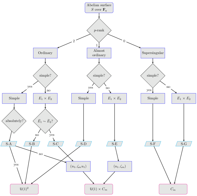
Theorem 1.0.4 (Abelian surfaces).
Let be an abelian surface over . Then has Serre–Frobenius group according to Figure 3. In particular, the possible options for the connected component of the identity , and the size of the cyclic component group are given below. Moreover, each one of these groups is realized for some prime power .
| 1,2,3,4,5,6,8,10,12,24 | |
| 1,2,3,4,6,8,12 | |
| 1 |
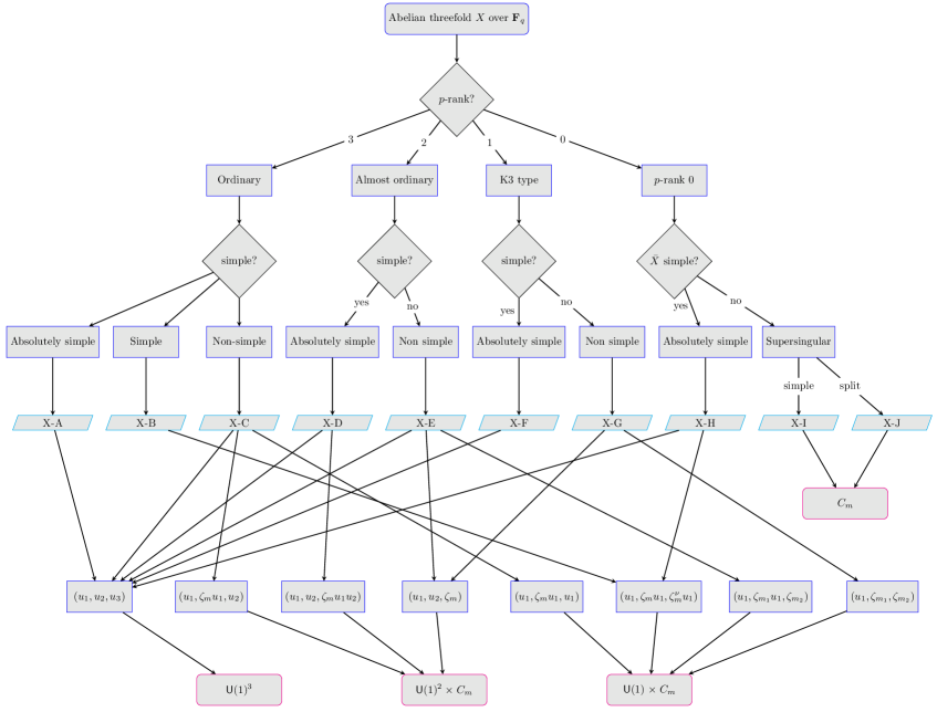
Theorem 1.0.5 (Abelian threefolds).
Let be an abelian threefold over . Then, has Serre–Frobenius group according to Figure 7. In particular, the possible options for the connected component of the identity, , and the size of the cyclic component group are given below. Moreover, each one of these groups is realized for some prime power .
| 1,2,3,4,5,6,7,8,9,10,12,14,15,18,20,24,28,30,36 | |
| 1,2,3,4,5,6,7,8,10,12,24 | |
| 1,2,3,4,6,8,12,24 | |
| 1 |
If is an odd prime, we have the following classification for simple ordinary abelian varieties; in the following theorem, we say that an abelian variety splits over a field extension if is isogenous over to a product of proper abelian subvarieties.
Theorem 1.0.6 (Prime dimension).
Let be a simple ordinary abelian variety defined over of prime dimension . Then, exactly one of the following conditions holds.
-
(1)
is absolutely simple.
-
(2)
splits over a degree extension of as a power of an elliptic curve, and .
-
(3)
splits over a degree extension of as a power of an elliptic curve, and . This case only occurs if is also a prime, i.e., if is a Sophie Germain prime.
1.1. Application to distributions of Frobenius traces
Our results can be applied to understanding the distribution of Frobenius traces of an abelian variety over as we range over finite extensions of the base field. Indeed, for each integer , we may rewrite Equation (2) as
denote the normalized Frobenius trace of the base change of an abelian variety to .
In [1], the authors study Jacobians of smooth projective genus curves with maximal angle rank111In their notation, this is the condition that the Frobenius angles are linearly independent modulo 1. and show that the sequence is equidistributed on with respect to an explicit measure. The Serre–Frobenius group enables us to remove the assumption of maximal angle rank.
Corollary 1.1.1.
Let be a -dimensional abelian variety defined over . Then, the sequence of normalized traces of Frobenius is equidistributed in with respect to the pushforward of the Haar measure on via the trace
| (3) |
The classification of the Serre–Frobenius groups in our theorems can be used to distinguish between the different Frobenius trace distributions occurring in each dimension.
Example 1.1.2.
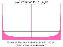
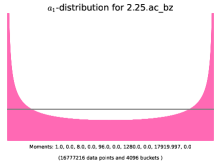
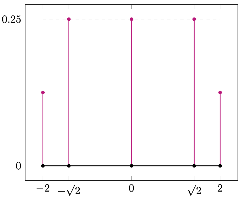
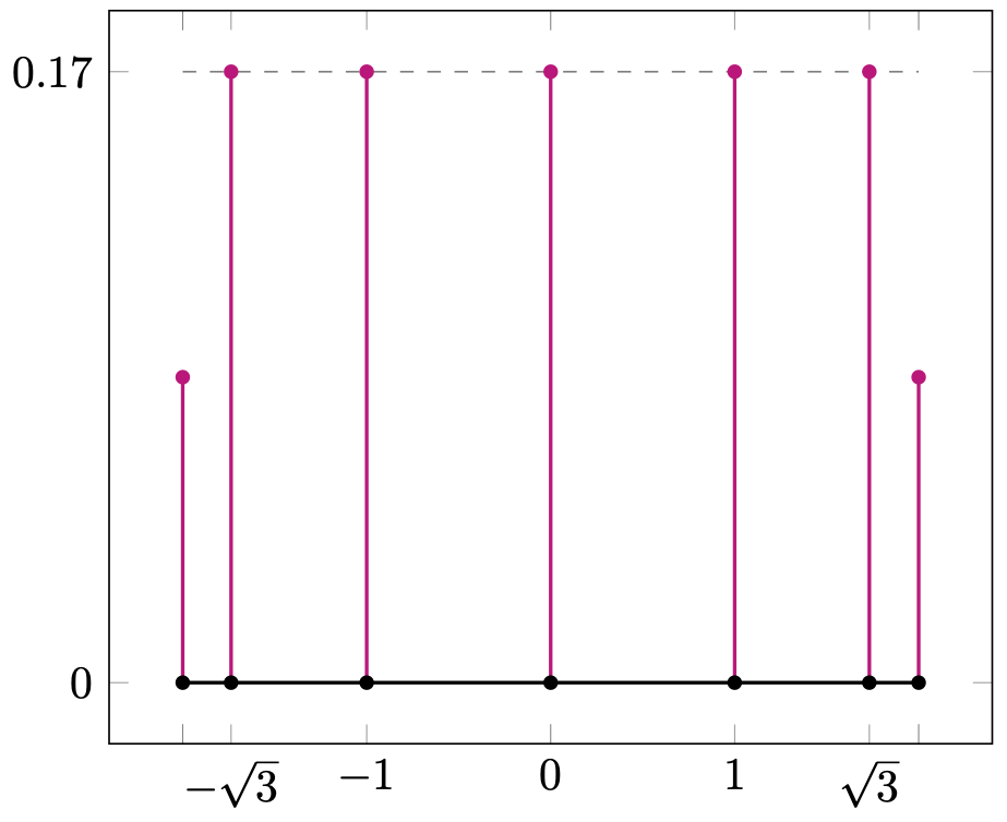
Let be a simple abelian surface over with Frobenius eigenvalues and suppose that is isogenous to for some ordinary elliptic curve . In this case, . Normalizing, and possibly after re-indexing, we see that either or . Since is simple and ordinary, the characteristic polynomial of Frobenius of is irreducible (see Remark 2.1.1), and we must have . The Serre–Frobenius groups of and are calculated as follows.
The sequence of normalized traces, henceforth referred to as the -sequence, is given by when is odd, and when is even. Extending the base field to yields the sequence of normalized traces . The data of the embedding precisely captures the (non-trivial) multiplicative relations between the Frobenius eigenvalues.
The sequence of normalized traces is equidistributed with respect to the pushforward of the Haar measure under the trace map given by , and similarly for . These can be computed explicitly for and as
| (4) |
where is the restriction of the Haar measure to , and is the Dirac measure supported at .
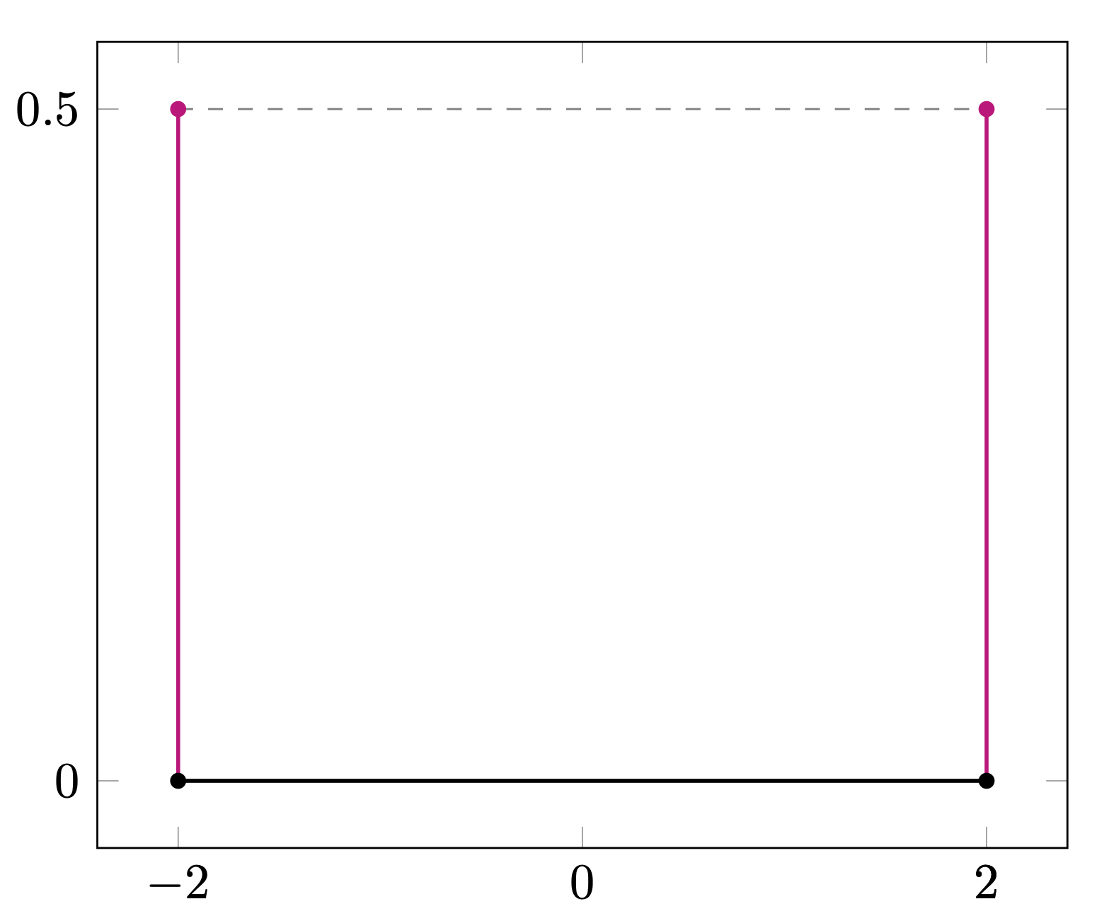
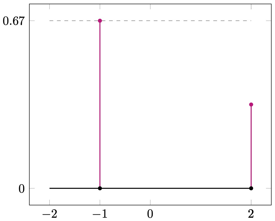
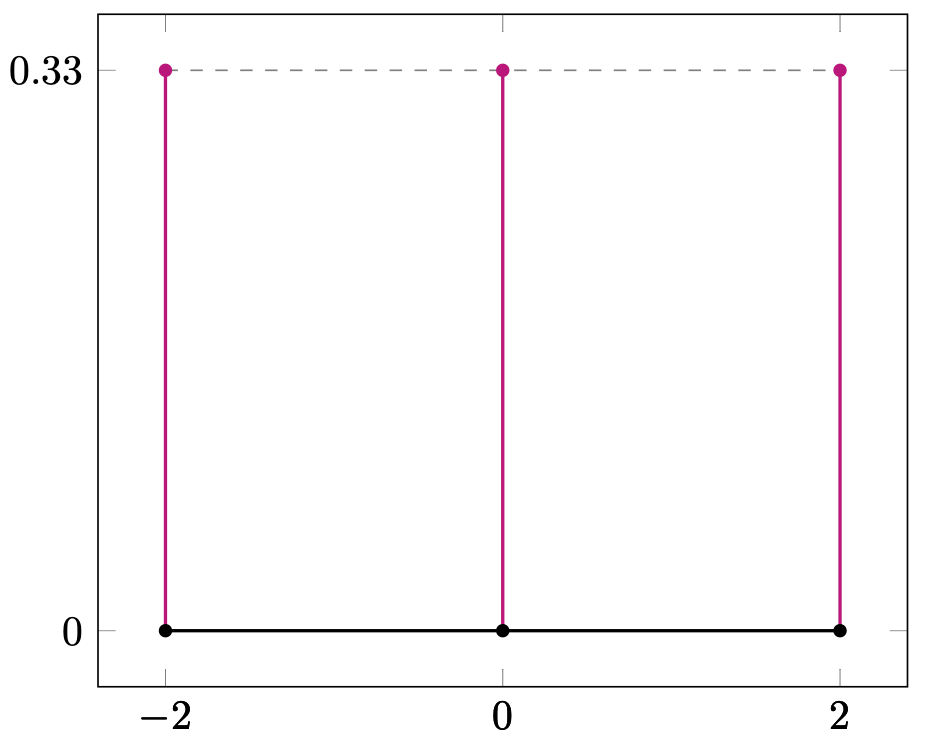
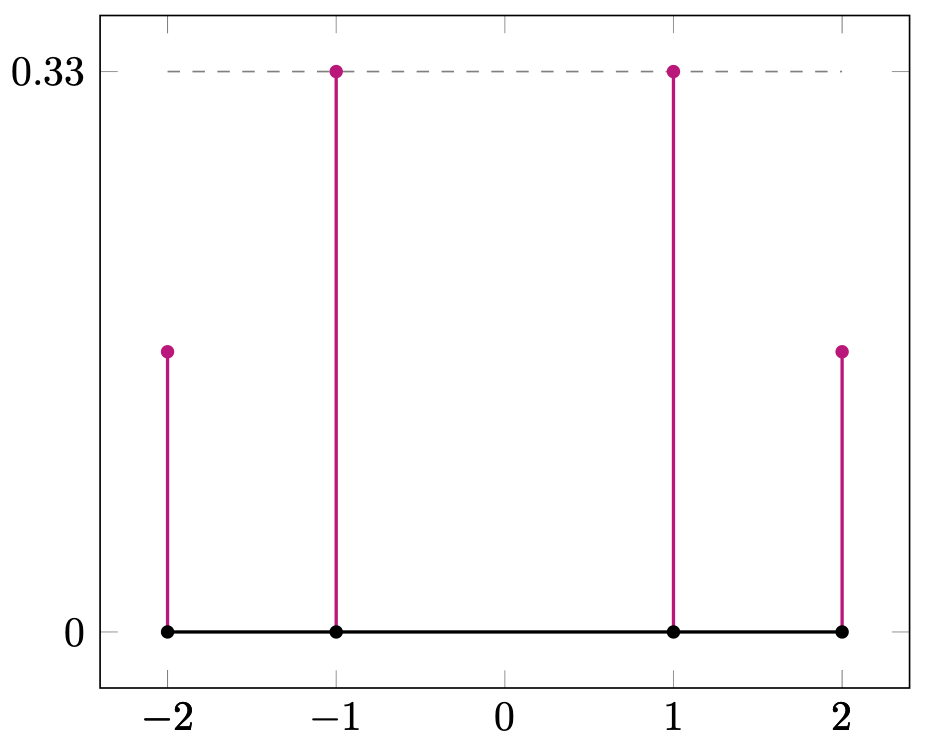
For instance, choose the surface to be in the isogeny class with LMFDB [17] label222Recall the labelling convention for isogeny classes of abelian varieties over finite fields in the LMFDB is g.q.iso where g is the dimension, q is the cardinality of the base field, and iso specifies the isogeny class by writing the coefficients of the Frobenius polynomial in base 26. 2.5.a_ab and Weil polynomial . This isogeny class is ordinary and simple, but not geometrically simple. Indeed, is in the isogeny class 2.25.ac_bz corresponding to the square of an ordinary elliptic curve. The corresponding -histograms describing the frequency of the sequence are depicted in Figure 1. Each graph represents a histogram of samples placed into buckets partitioning the interval . The vertical axis has been suitably scaled, with the height of the uniform distribution, , indicated by a gray line.
1.2. Relation to other work
The reason for adopting the name “Serre–Frobenius group” is that the Lie group is closely related to Serre’s Frobenius torus [27], as explained in Remark 2.3.4.
1.2.1. Angle rank
In this article, we study multiplicative relations between Frobenius eigenvalues, a subject studied extensively by Zarhin [37, 38, 16, 39, 40]. Our classification relies heavily on being able to understand multiplicative relations in low dimension, and we use results of Zarhin in completing parts of it. The number of multiplicative relations is quantified by the angle rank, an invariant studied in [8], [7] for absolutely simple abelian varieties by elucidating its interactions with the Galois group and Newton polygon of the Frobenius polynomial. We study the angle rank as a stepping stone to classifying the full Serre–Frobenius group. While our perspective differs from that in [8], the same theme is continued here: the Serre–Frobenius groups depend heavily on the Galois group of the Frobenius polynomial. It is worth noting that here that the results about the angle rank in the non-absolutely simple case cannot be pieced together by knowing the results in the absolutely simple cases (for instance, see Zywina’s exposition of Shioda’s example [42, Remark 1.16]).
1.2.2. Sato–Tate groups
The Sato–Tate group of an abelian variety defined over a number field controls the distribution of the Frobenius of the reduction modulo prime ideals, and it is defined via its -adic Galois representation (see [30, Section 3.2]). The Serre–Frobenius group can also be defined via -adic representations in an analogous way: it is conjugate to a maximal compact subgroup of the image of Galois representation , where is the -adic Tate vector space. Therefore it is natural to expect that the Sato–Tate and the Serre–Frobenius group are related to each other. The following observations support this claim:
-
•
Assuming standard conjectures, the connected component of the identity of the Sato–Tate group can be recovered from knowing the Frobenius polynomial at two suitably chosen primes ([42, Theorem 1.6]).
-
•
Several abelian Sato–Tate groups (see [10, 11]) appear as Serre–Frobenius groups of abelian varieties over finite fields. The ones with maximal angle rank are as below.
-
–
is the Sato–Tate group of an elliptic curve with complex multiplication over any number field that contains the CM field (see 1.2.B.1.1a). It is also the Serre–Frobenius group of any ordinary elliptic curve (see Figure 2(a)), and the -moments coincide.
-
–
is the Sato–Tate group of weight 1 and degree 4 (see 1.4.D.1.1a). It is also the Serre–Frobenius group of an abelian surface with maximal angle rank (see Figure 4(a)), and the -moments coincide.
-
–
is the Sato–Tate group of weight 1 and degree 6 (see 1.6.H.1.1a). It is also the Serre-Frobenius group of abelian threefolds with maximal angle rank (see Figure 8), and the -moments coincide.
-
–
1.3. Outline
In Section 2, we give some background on abelian varieties over finite fields, expand on the definition of the Serre–Frobenius group, and describe how it controls the distribution of traces of high powers of Frobenius. In Section 3, we prove some preliminary results on the geometric isogeny types of abelian varieties of dimension and odd prime. We also recall some results about Weil polynomials of supersingular abelian varieties, and Zarhin’s notion of neatness. In Section 3.2, we discuss the classification in the case of simple ordinary abelian varieties of odd prime dimension. In Section 4, Section 5, and Section 6, we give a complete classification of the Serre–Frobenius group for dimensions 1, 2, and 3 respectively. A list of tables containing different pieces of the classification follows this section.
1.4. Notation
Throughout this paper, will denote a -dimensional abelian variety over a finite field of characteristic . The polynomial will denote the characteristic polynomial of the -Frobenius endomorphism acting on the Tate module of , and its minimal polynomial. The set of roots of is denoted by . We usually write for the Frobenius eigenvalues, where . In the case that is a power of , we will denote this power by (See 2.1). The subscript will denote the base change of any object or map to . The group will denote the multiplicative group generated by the normalized eigenvalues of Frobenius, its rank and the order of its torsion subgroup. The group will denote the multiplicative group generated by . In Section 5, will be used to denote an abelian surface, while in Section 6, will be used to denote a threefold.
2. Frobenius multiplicative groups
In this section we introduce the Serre–Frobenius group of and explain how it is related to Serre’s theory of Frobenius tori [27]. We do this from the perspective of the theory of algebraic groups of multiplicative type, as in [19, Chapter 12]. We start by recalling some facts about abelian varieties over finite fields.
2.1. Background on Abelian varieties over finite fields
Fix a dimensional abelian variety over . A -Weil number is an algebraic integer such that for every embedding . Let denote the characteristic polynomial of the Frobenius endomorphism acting on the -adic Tate module of . The polynomial is monic of degree , and Weil [34] showed that its roots are -Weil numbers; we denote the set of roots of by with for . The seminal work of Honda [13] and Tate [31, 32] classifies the isogeny decomposition type of in terms of the factorization of . In particular, if is simple, we have that where is the minimal polynomial of the Frobenius endomorphism and is the degree, i.e., the square root of the dimension of the central simple algebra over its center. The Honda–Tate theorem gives a bijective correspondence between isogeny classes of simple abelian varieties over and conjugacy classes of -Weil numbers, sending the isogeny class determined by to the set of roots . Further, the isogeny decomposition can be read from the factorization .
Writing , the -Newton polygon of is the lower convex hull of the set of points where is the -adic valuation normalized so that . The Newton polygon is isogeny invariant. Define the -rank of as the number of slope segments of the Newton polygon. An abelian variety is called ordinary if it has maximal -rank, i.e., its -rank is equal to . It is called almost ordinary if it has -rank ; equivalently, the set of slopes of its Newton polygon is and the slope has length . An abelian variety is called supersingular if all the slopes of the Newton polygon are equal to . The field is the splitting field of the Frobenius polynomial. By definition, the Galois group acts on the roots by permuting them.
Remark 2.1.1.
When an abelian variety over is simple and ordinary, then is irreducible and its endomorphism algebra is a field ([33, Theorem 7.2]).
Notation.
Whenever is fixed or clear from context, we will omit the subscript corresponding to it from the notation described above. In particular, we will use and instead of and .
2.2. Angle groups
Denote by the multiplicative subgroup of generated by the set of Frobenius eigenvalues , and let for every . Since is a permutation of , the set is a set of generators for ; that is, every can be written as
| (5) |
for some .
Since is a subgroup of , it is naturally a -module. However, this perspective is not necessary for our applications. This group is denoted as in [42].
Definition 2.2.1.
We define the angle group of to be , the multiplicative subgroup of generated by the unitarized eigenvalues }. When is fixed, for every we abbreviate .
Definition 2.2.2.
The angle rank of an abelian variety is the rank of the finitely generated abelian group . It is denoted by . The angle torsion order is the order of the torsion subgroup of , so that .
The angle rank is by definition an integer between and . When , there are no multiplicative relations among the normalized eigenvalues. In other words, there are no additional relations among the generators of apart from the ones imposed by the Weil conjectures. If is absolutely simple, the maximal angle rank condition also implies that the Tate conjecture holds for all powers of (see Remark 1.3 in [8]). On the other extreme, if and only if is supersingular (See Example 5.1 [7]).
Remark 2.2.3.
The angle rank is invariant under base extension: for every . Indeed, any multiplicative relation between is a multiplicative relation between . We have that for every positive integer . In particular, where is the angle torsion order of .
Example 2.2.4 (Extension and restriction of scalars).
Let be an abelian variety with Frobenius polynomial and angle group . Then, the extension of scalars has Frobenius polynomial and angle group . On the other hand, if is an abelian variety for some , and is the Weil restriction of to , then and . See [6].
2.3. The Serre–Frobenius group
For every locally compact abelian group , denote by its Pontryagin dual; this is the topological group of continuous group homomorphisms . It is well known that gives an anti-equivalence of categories from the category of locally compact abelian groups to itself. Moreover, this equivalence preserves exact sequences, and every such is canonically isomorphic to its double dual via the evaluation isomorphism. See [23] for the original reference and [20] for a gentle introduction.
Recall that we defined the Serre–Frobenius group of as the topological group generated by the matrix inside of (see 1.0.1).
Remark 2.3.1.
The group embeds into as a maximal torus via , so a different choice of indexing of the Frobenius eigenvalues yields a conjugate subgroup , where is an element of the Weyl group . This Weyl group is isomorphic to the group of signed permutation matrices; the generic Galois group of a complex multiplication polynomial of degree .
Notation.
In light of Remark 2.3.1, we identify with the group
and the vector with the matrix . The embedding of into is completely determined by the topological generator of , a vector of normalized Frobenius eigenvalues. We will represent the embedding of into (up to conjugation) by giving the topological generator of the Serre–Frobenius group.
The following lemma will help us identify the isomorphism class of as a compact abelian group.
Lemma 2.3.2.
The Serre–Frobenius group of an abelian variety has character group . In particular, canonically via the evaluation isomorphism.
Proof.
We have an injection given by mapping to the character that maps the topological generator to . To see that this map is surjective, observe that by the exactness of Pontryagin duality, the inclusion induces a surjection . Explicitly, this tells us that every character of is given by for some . By continuity, every character of is completely determined by . In particular, we have that . ∎
The following theorem should be compared to [30, Theorem 3.12]
Theorem 2.3.3 (Theorem 1.0.2).
Let be an abelian variety defined over . Then
where is the angle rank and is the angle torsion order. Furthermore, the connected component of the identity is
Proof.
Since every finite subgroup of is cyclic, the torsion part of the finitely generated group is generated by some primitive -th root of unity . The group is torsion free by Remark 2.2.3. We thus have the split short exact sequence
| (6) |
After dualizing, we get:
| (7) |
We conclude that and . ∎
Remark 2.3.4.
By definition, is the image of under the radial projection . Thus, we have a short exact sequence
| (8) |
which is split by the section . The kernel is free of rank and contains the group . The relation between the Serre–Frobenius group and Serre’s Frobenius Torus (see [27, Volume IV, 133.], [4, Section 3]) can be understood via their character groups.
-
•
The (Pontryagin) character group of is .
-
•
The (algebraic) character group of the Frobenius torus of is the torsion free part of .
2.4. Equidistribution results
Let be a measure space in the sense of Serre (see Appendix A.1 in [26]). Recall that a sequence is -equidistributed if for every continuous function we have that
| (9) |
In our setting, will be a compact abelian Lie group with probability Haar measure . We have the following lemma.
Lemma 2.4.1.
Let be a compact group, and . Let be the closure of the group generated by . Then, the sequence is equidistributed in with respect to the Haar measure .
Proof.
For a non-trivial character , the image of the generator is non-trivial. We see that
both when has finite or infinite order. The latter case follows from Weyl’s equidistribution theorem in . The result follows from Lemma 1 in [26, I-19] and the Peter–Weyl theorem. ∎
Corollary 2.4.2 (1.1.1).
Let be a -dimensional abelian variety defined over . Then, the sequence of normalized traces of Frobenius is equidistributed in with respect to the pushforward of the Haar measure on via
Proof.
By Lemma 2.4.1, the sequence is equidistributed in with respect to the Haar measure . By definition, the sequence is equidistributed with respect to the pushforward measure, and it is invariant under relabelling of the Frobenius eigenvalues. ∎
Remark 2.4.3 (Maximal angle rank).
When has maximal angle rank , the Serre–Frobenius group is the full torus , and the sequence of normalized traces of Frobenius is equidistributed with respect to the pushforward of the measure ; which we denote by following the notation333Beware of the different choice of normalization. We chose to use the interval instead of to be able to compare our distributions with the Sato–Tate distributions of abelian varieties defined over number fields. in [1].
3. Preliminary Results
For this entire section, we let be an abelian variety over , where for some prime . Recall from Section 1 that an abelian variety splits over a field extension if and , i.e., if obtains at least one isogeny factor after extending scalars to . We say that splits completely over if , where each is an absolutely simple abelian variety defined over . In other words, acquires its geometric isogeny decomposition over . We define the splitting degree of to be the minimal positive integer such that splits completely over .
3.1. Geometric products of elliptic curves
We begin by stating an important lemma, attributed to Bjorn Poonen in [15].
Lemma 3.1.1 (Poonen).
If are pairwise geometrically non-isogenous elliptic curves over , then their eigenvalues of Frobenius are multiplicatively independent.
In fact, for abelian varieties that split completely as products of elliptic curves, we can explicitly describe the Serre–Frobenius group.
Lemma 3.1.2.
Let be an abelian variety that splits over as a power of an ordinary elliptic curve, where is the splitting degree of . Then, . Furthermore, if , then
with -th roots of unity whose orders have least common multiple . In particular, when is simple then all the are distinct, primitive and .
Proof.
Angle rank is invariant under base change, so . It remains to show that the angle torsion order equals . If , then and there is nothing to show. Assume that . Since , we have that . If we denote by and the Frobenius eigenvalues of and respectively, we have that . Possibly after relabelling, we have that for , where the ’s are -th roots of unity and the minimality of ensures that the lcm of the orders of the ’s is . This shows that , so that . On the other hand, we have that is connected. This implies that and we conclude that . Assume now is simple, then is irreducible and hence has no repeated roots, and thus for every , and every is primitive. This shows that the set has elements, and therefore . ∎
Lemma 3.1.3.
Let be an abelian variety over such that is supersingular with angle torsion order and splits over as the power of an ordinary elliptic curve, where is the splitting degree of . Then, and . Furthermore,
where denotes the (pointwise) complex conjugate of , and similarly for .
Proof.
From Lemma 3.1.2, we see that , where is a normalized Frobenius eigenvalue of and all the other roots can be written as with It follows that so that and . Furthermore, is generated by for some with and . ∎
Lemma 3.1.4.
Let be an ordinary abelian variety defined over such that is geometrically isogenous to a product of elliptic curves. Let be the splitting degree of , and write with not geometrically isogenous to for . Then . Moreover, we can describe the embedding of as follows:
-
(1)
Let be the smallest positive integer such that decomposes into pairwise non-geometrically isogenous factors.
-
(2)
Let be the splitting degree of , so that .
Then, and
where each is as in Lemma 3.1.2, and denotes the (pointwise) complex conjugate of .
Proof.
This follows from combining Lemma 3.1.1 with the fact that the Serre–Frobenius group of is connected over an extension of degree . The proof then proceeds as in Lemma 3.1.2. ∎
3.2. Splitting of simple ordinary abelian varieties of odd prime dimension
In this section, we analyze the splitting behavior of simple ordinary abelian varieties of prime dimension . Our first result is analogous to [14, Theorem 6] for odd primes.
Theorem 3.2.1 (Theorem 1.0.6).
Let be a simple ordinary abelian variety defined over of prime dimension . Then, exactly one of the following conditions holds.
-
(1)
is absolutely simple.
-
(2)
splits over a degree extension of as a power of an elliptic curve, and .
-
(3)
splits over a degree extension of as a power of an elliptic curve, and . This case only occurs if is also a prime, i.e., if is a Sophie Germain prime.
Furthermore, in (2) and (3), we have that
with distinct primitive -th roots of unity, for and respectively.
Proof.
Let be a Frobenius eigenvalue of , and denote by the number field generated by . Since is ordinary, is a CM-field over for every positive integer , and is irreducible and therefore . Suppose that is not absolutely simple, and let be the smallest positive integer such that splits; by [14, Lemma 4] this is also the smallest such that . Since is also a CM field, it is necessarily an imaginary quadratic number field.
Observe first that must be odd. Indeed, if was even, then and . This contradicts the fact that , since is an odd prime. By [14, Lemma 5], there are two possibilities:
-
(i)
,
-
(ii)
.
If (i) holds and , we conclude that and . In this case, the minimal polynomial of has degree 2 and is of the form . Note that and are distinct, since is ordinary. Thus, and must split over a degree extension as the power of an ordinary elliptic curve.
If (ii) holds, we have that . Since is odd and takes even values, we have two possible options: either or . If , then which contradicts the fact that is a degree extension of . Therefore, necessarily, , and Recall from elementary number theory that the solutions to this equation are or for a Sophie Germain prime.
-
•
() In this case, (ii) only occurs when is prime.
-
•
() In this case, either or . To conclude the proof, we show that does not occur. More precisely, we will show that if splits over a degree extension, it splits over a degree extension as well. In fact, suppose that for a primitive th root of unity. The subfield is the only imaginary quadratic subfield of , so if a power of does not generate , it must lie in . Suppose lies in . Let be the generator of sending to . The minimal polynomial of over divides , so for some , and . Since the product of the three conjugates of over must lie in , we have that , which implies that and we conclude that splits over a degree- extension of the base field.
The statement about the structure of the Serre–Frobenius group follows from Lemma 3.1.2. ∎
We thank Everett Howe for explaining to us why the case above does not occur.
3.3. Zarhin’s notion of neatness
In this section we discuss Zarhin’s notion of neatness, a useful technical definition closely related to the angle rank. Define
| (10) |
Note that according to our numbering convention, we have that for every .
Definition 3.3.1 (Zarhin).
Let be an abelian variety defined over . We say that is neat if it satisfies the following conditions:
-
(Na)
is torsion free.
-
(Nb)
For every function satisfying
then for every .
Remarks 3.3.2.
-
(3.3.2.a)
If is supersingular and is torsion free, then is neat. Indeed, in this case we have that and condition (Nb) is trivially satisfied.
-
(3.3.2.b)
Suppose that the Frobenius eigenvalues of are distinct and not supersingular. Some base extension of is neat if and only if has maximal angle rank.
-
(3.3.2.c)
In general, maximal angle rank always implies neatness.
3.4. Supersingular Serre–Frobenius groups
Recall that a -Weil number is called supersingular if is a root of unity. In [41, Proposition 3.1], Zhu classified the minimal polynomials of supersingular -Weil numbers. Let denote the -th cyclotomic polynomial, the Euler totient function, and the Jacobi symbol. Then the possibilities for the minimal polynomials of supersingular -Weil numbers are given in Table 2.
| Type | Roots | |||
| Z-1 | Even | - | ||
| Z-2 | Odd | |||
| Z-3 | Odd |
Notation (Table 2).
In case (Z-1), is any positive integer. In cases (Z-2) and (Z-3), additionally satisfies , and . The symbol denotes the a primitive -th root of unity. Note that in this case, . Following the notation in [29], given a polynomial for some field , and a constant , let
Given any supersingular abelian variety defined over , the Frobenius polynomial is a power of the minimal polynomial , and this minimal polynomial is of type (Z-1), (Z-2), or (Z-3) as above. We say that is of type Z-i if the minimal polynomial is of type (Z-i) for .
Since is finite in the supersingular case, we have that . Furthermore, we have that
with ’s being -th roots of unity, whose orders have least common multiple . In particular, we can read off the character group from the fourth column in Table 2. For instance, if and is even, then we have a polynomial of type Z-1, and the Serre–Frobenius group is isomorphic to . On the other hand, if and we have a polynomial of type Z-2, then the Serre–Frobenius group is isomorphic to . Given a -Weil polynomial with roots , the associated normalized polynomial is the monic polynomial with roots . Table 2 allows us to go back and forth between -Weil polynomials and the normalized polynomials .
-
•
If is the minimal polynomial of a supersingular -Weil number of type Z-1, the normalized polynomial is the cyclotomic polynomial . Conversely, we have that .
-
•
If is the minimal polynomial of a supersingular -Weil number of type Z-2, the normalized polynomial is the polynomial . Conversely, .
4. Elliptic Curves
The goal of this section is to prove Theorem 1.0.3. Furthermore, we give a thorough description of the set of possible orders for the supersingular Serre–Frobenius groups in terms of and .
The isogeny classes of elliptic curves over were classified by Deuring [5] and Waterhouse [33, Theorem 4.1]. Writing the characteristic polynomial of Frobenius as , the Weil bounds give . Conversely, the integers satisfying that correspond to the isogeny class of an elliptic curve are the following.
Theorem 4.0.1 ([28, Theorem 2.6.1]).
Let be a prime and . Let satisfy .
-
(1)
If , then is the trace of Frobenius of an elliptic curve over . This is the ordinary case.
-
(2)
If , then is the trace of Frobenius of an elliptic curve over if and only if one of the following holds:
-
(i)
is even and ,
-
(ii)
is even and with ,
-
(iii)
is even and with ,
-
(iv)
is even and with ,
-
(v)
is odd and ,
-
(vi)
is odd, with .
-
(vii)
is odd, with .
This is the supersingular case.
-
(i)
In the ordinary case, the normalized Frobenius eigenvalue is not a root of unity, and thus . In the supersingular case, the normalized Frobenius eigenvalue is a root of unity, and thus is cyclic, with equal to the order of . For each value of and in Theorem 4.0.1 part (2), we get a right triangle of hypotenuse of length and base , from which we can deduce the angle and thus the order of the corresponding root of unity . We thus obtain Theorem 1.0.3 as a restatement of Theorem 4.0.1.
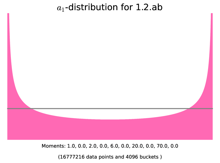
There are eight Serre–Frobenius groups for elliptic curves, sumarized in Table 3, and they correspond to eight possible Frobenius distributions of elliptic curves over finite fields. For ordinary elliptic curves (as explained in Section 1), the sequence of normalized traces is equidistributed in the interval with respect to the measure (Equation 1) obtained as the pushforward of the Haar measure under . See Figure 2(a).
The remaining seven Serre–Frobenius groups are finite and cyclic; they correspond to supersingular elliptic curves. For a given , denote by the measure obtained by pushforward along of the normalized counting measure,
| Theorem 4.0.1 | Generator | Example | Figure 2 | ||||
| (1) | - | - | 1.2.ab | 2(a) | |||
| 2-2(i) | - | Even | 1.4.ae | 2(b) | |||
| 2-2(i) | - | Even | - | 1.4.e | 2(c) | ||
| 2-2(iii) | Even | 1.4.c | 2(d) | ||||
| 2-2(iv) | Even | 1.4.a | 2(e) | ||||
| 2-2(v) | - | Odd | 1.2.a | 2(e) | |||
| 2-2(ii) | Even | 1.4.ac | 2(f) | ||||
| 2-2(vi) | 2 | Odd | 1.2.ac | 2(g) | |||
| 2-2(vii) | 3 | Odd | 1.3.ad | 2(h) |
5. Abelian Surfaces
The goal of this section is to classify the possible Serre–Frobenius groups of abelian surfaces (Theorem 1.0.4). The proof is a careful case-by-case analysis, described by Flowchart 3.
We separate our cases first according to -rank, and then according to simplicity. In the supersingular and almost ordinary cases this stratification is enough. In the ordinary case, we have to further consider the geometric isogeny type of the surface. When the angle rank is , the Serre–Frobenius group is the full torus . When the angle rank is , the Serre–Frobenius group is isomorphic to but there are two non-conjugate ways to embed into ; these are determined by the topological generator of the group, which can be either or .
5.1. Simple ordinary surfaces
We restate a theorem of Howe and Zhu in our notation.
Theorem 5.1.1 ([14, Theorem 6]).
Suppose that is the Frobenius polynomial of a simple ordinary abelian surface defined over . Then, exactly one of the following conditions holds.
-
(a)
is absolutely simple.
-
(b)
and splits over a quadratic extension.
-
(c)
and splits over a cubic extension.
-
(d)
and splits over a quartic extension.
-
(e)
and splits over a sextic extension.
Lemma 5.1.2 (Node S-A in Figure 3).
Let be a simple ordinary abelian surface over . Then, exactly one of the following conditions holds.
-
(a)
is absolutely simple and .
-
(b)
splits over a quadratic extension and .
-
(c)
splits over a cubic extension and .
-
(d)
splits over a quartic extension and .
-
(e)
splits over a sextic extension and .
In cases (b)-(e), we have that , for some primitive -th root of unity .
Proof.
-
(a)
From [40, Theorem 1.1], we conclude that some finite base extension of an absolutely simple abelian surface is neat and therefore has maximal angle rank by Remark (3.3.2.c). Alternatively, this also follows from the proof of [1, Theorem 2] for Jacobians of genus 2 curves, which generalizes to any abelian surface. Theorem 1.0.2 then implies that .
-
(b,c,d,e)
Denote by the splitting degree of . By Theorem 5.1.1 we know that . Let be a Frobenius eigenvalue of . From [14, Lemma 4] and since is ordinary, we have that . In particular, the minimal polynomial of is quadratic, and . This implies that , so that (up to relabelling) there is a primitive444Note that must be primitive, since otherwise, would split for some , contradicting the minimality of . -th root of unity such that . It follows that
and embeds diagonally in .
∎


Notation.
In Table 4, the Splitting type title refers to that of the abelian variety , the class title refers to the Serre–Frobenius group , and the Generator title refers to the topological generator of ; which precisely and succinctly captures the data of the embedding of the Serre–Frobenius group into the ambient unitary symplectic group. We will follow the same conventions in the following tables.
5.2. Non-simple ordinary surfaces
Let be a non-simple ordinary abelian surface defined over . Then is isogenous to a product of two ordinary elliptic curves . As depicted in Figure 3, we consider two cases:
-
(S-B)
and are not isogenous over .
-
(S-C)
and become isogenous over some base extension , for .
The Serre-Frobenius groups corresponding to these isogeny decomposition types are sumarized in Table 5. The proof of the following lemma is a straightforward application of Lemma 3.1.1.
Lemma 5.2.1 (Node S-B in Figure 3).
Let be an abelian surface defined over such that is isogenous to , for and geometrically non-isogenous ordinary elliptic curves. Then has maximal angle rank and .
Lemma 5.2.2 (Node S-C in Figure 3).
Let be an abelian surface defined over such that is isogenous to , for and geometrically isogenous ordinary elliptic curves. Then has angle rank and for . Furthermore, is precisely the degree of the extension of over which and become isogenous.
Proof.
Let and denote the Frobenius eigenvalues of and respectively. Let be the smallest positive integer such that . From Lemma 3.1.2, we immediately have that , where . In order to find the value of , observe that , from which we may assume, possibly after relabelling, that for some primitive -th root of unity . Since the curves and are ordinary, the number fields and are imaginary quadratic and . Hence, and thus ; therefore . Finally, we have by definition that . ∎


5.3. Simple almost ordinary surfaces
In [16] Lenstra and Zarhin carried out a careful study of the multiplicative relations of Frobenius eigenvalues of simple almost ordinary varieties (see section 2.1 for the definition), which was later generalized in [8]. In particular, they prove that even dimensional simple almost ordinary abelian varieties have maximal angle rank ([16, Theorem 5.8]). Since every abelian surface of -rank is almost ordinary, their result allows us to deduce the following.
Lemma 5.3.1 (Node S-D in Figure 3).
Let be a simple and almost ordinary abelian surface defined over . Then has maximal angle rank and .
5.4. Non-simple almost ordinary surfaces
If is almost ordinary and not simple, then is isogenous to the product of an ordinary elliptic curve and a supersingular elliptic curve . The corresponding Serre-Frobenius groups are sumarized in Table 6.
Lemma 5.4.1 (Node S-E in Figure 3).
Let be a non-simple almost ordinary abelian surface defined over . Then has angle rank and angle torsion order . Furthermore, .
Proof.
Let be an ordinary elliptic curve and a supersingular elliptic curve such that . By Lemma 3.1.3, with in the list of possible orders of Serre–Frobenius groups of supersingular elliptic curves. ∎


5.5. Simple supersingular surfaces
Since every supersingular abelian variety is geometrically isogenous to a power of an elliptic curve, the Serre–Frobenius group only depends on the splitting degree. We separate our analysis into the simple and non-simple cases.
The classification of Frobenius polynomials of supersingular abelian surfaces over finite fields was completed by Maisner and Nart [18, Theorem 2.9] building on work of Xing [36] and Rück [24]. Denoting by the isogeny class of abelian surfaces over with Frobenius polynomial , the following lemma gives the classification of Serre–Frobenius groups of simple supersingular surfaces.
Lemma 5.5.1 (Node S-F in Figure 3).
Let be a simple supersingular abelian surface defined over . The Serre–Frobenius group of is classified according to Table 7.
| Type | Example | ||||||
| even | Z-1 | 2.4.a_a | |||||
| odd | Z-2 | 2.3.a_a | |||||
| - | odd | Z-2 | 2.2.a_c | ||||
| even | Z-1 | 2.4.a_ae | |||||
| odd | Z-2 | 2.2.a_ac | |||||
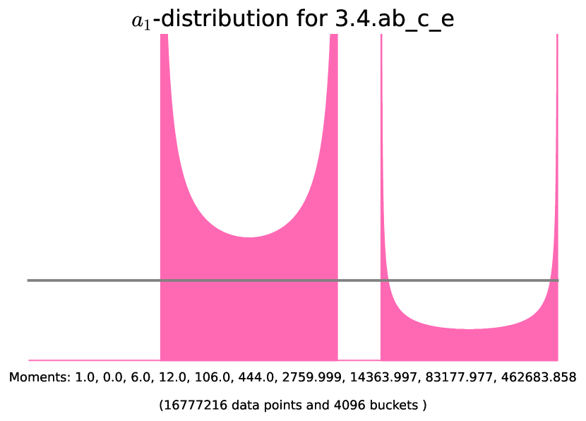
| even | Z-1 | 2.4.c_e | |||||
| even | Z-1 | 2.4.ac_e | |||||
| odd | Z-3 | 2.5.f_p | |||||
| odd | Z-3 | 2.5.af_p | |||||
| odd | Z-3 | 2.2.c_c | |||||
| odd | Z-3 | 2.2.ac_c | |||||
| - | odd | Z-2 | 2.2.a_ae | ||||
| even | Z-1 | 2.25.a_by | |||||
| even | Z-1 | 2.49.o_fr | |||||
| even | Z-1 | 2.49.ao_fr |
The notation for polynomials of type Z-3 is taken from [29], where the authors classify simple supersingular Frobenius polynomials for . We have
| (11) | ||||
| (12) |
We exhibit the proof of the second line in Table 7 for exposition. The remaining cases can be checked similarly. If , and is an odd power of : then, and . Thus is generated by a primitive 8th root of unity.
5.6. Non-simple supersingular surfaces
If is a non-simple supersingular surface, then is isogenous to a product of two supersingular elliptic curves and . If and denote the torsion orders of and respectively, then the extension over which and become isogenous is precisely . Thus, we have the following result, depending on the values of as in Table 3.
Lemma 5.6.1 (Node S-G in Figure 3).
Let be a non-simple supersingular abelian surface defined over . Then has angle rank and for in the set described in Table 8.
| Even | - | |
| Even | ||
| Even | ||
| Odd | - | |
| Odd | ||
| Odd |
6. Abelian Threefolds
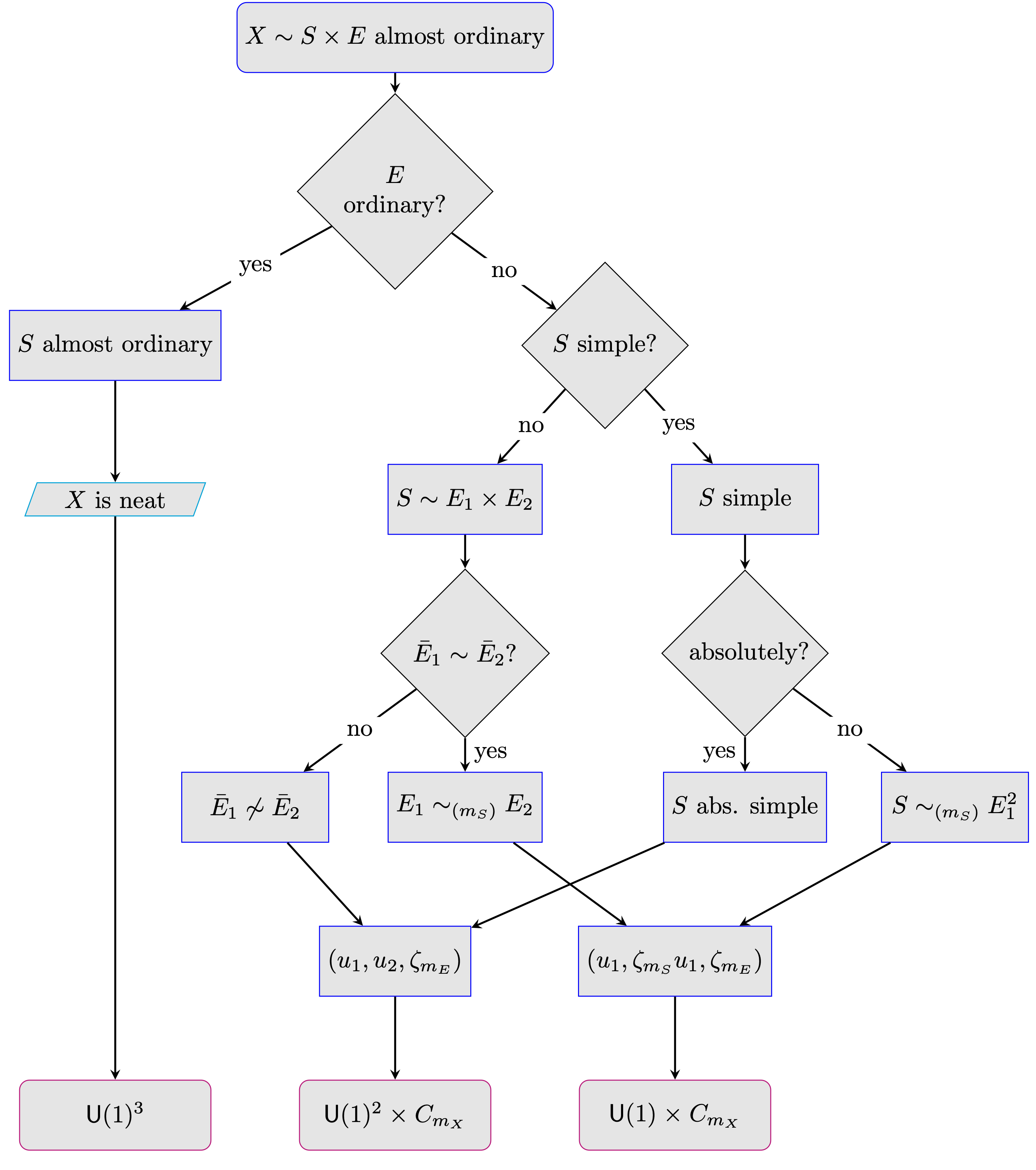
In this section, we classify the Serre–Frobenius groups of abelian threefolds (see Figure 7). Let be an abelian variety of dimension defined over . For our analysis, we will first stratify the cases by -rank and then by simplicity. Before we proceed, we make some observations about simple threefolds that will be useful later.
6.1. Simple abelian threefolds
If is a simple abelian threefold, there are only two possibilities for the Frobenius polynomial :
| (13) | ||||
| (14) |
Indeed, if were a linear or cubic polynomial, it would have a real root . By an argument of Waterhouse [33, Chapter 2], the -Weil numbers must come from simple abelian varieties of dimension 1 or 2. Further, Xing [35] showed that Equation 14 can only occur in very special cases.
Theorem 6.1.1 ([35], [12, Proposition 1.2]).
Let be a simple abelian threefold over . Then, if and only if divides and with .
When is a cube as above, since , the -adic valuation of its middle coefficient is the same as that of , which in turn is . Thus, is non-supersingular of -rank and its Newton Polygon has slopes . Furthermore, every simple abelian threefold is either absolutely simple or geometrically isogenous to the cube of an elliptic curve. Thus, we have the following.
Lemma 6.1.2.
If is an abelian threefold defined over that is not ordinary or supersingular, then is simple if and only if it is absolutely simple.
Proof.
Assume is a simple abelian threefold that is not ordinary or supersingular. Assume also that is not absolutely simple. Let be the splitting degree of . Recall that since is simple, one either has or , where is irreducible of even degree. We will show that in each case , contradicting the assumption that is not ordinary or supersingular.
Assume , then . Observe that necessarily has an elliptic curve as an isogeny factor. Then , a quadratic polynomial, must divide , and we conclude . Thus .
Assume instead that , that is, is irreducible. Therefore is a degree extension and . Then by [3, Theorem 1.3.1.1] is isotypic, so that . ∎
In each case of the classification that follows, we will denote by , the set of possible angle torsion orders that occur for that case. When we want to emphasize the dependence on the prime and the power , we will denote this by .
6.2. Simple ordinary threefolds
In this section, will denote a simple ordinary abelian threefold defined over . The corresponding Serre-Frobenius groups are sumarized in Table 9.
As a corollary to Theorem 3.2.1, we have the following.
Proposition 6.2.1.
Let be a simple ordinary abelian threefold defined over . Then, exactly one of the following conditions is satisfied.
-
(1)
is absolutely simple.
-
(2)
splits over a degree extension and .
-
(3)
splits over a degree extension and the number field of is .
Lemma 6.2.2 (Node X-A in Figure 7).
Let be an absolutely simple abelian threefold defined over . Then has maximal angle rank and .
Proof.
Let be the order of the torsion subgroup of . By [40, Theorem 1.1], we have that is neat. Since is ordinary and simple, its Frobenius eigenvalues are distinct and non-real. Remark (3.3.2.b) implies that has maximal angle rank. Since angle rank is invariant under base extension (Remark 2.2.3) we have that as we wanted to show. ∎
Lemma 6.2.3 (Node X-B in Figure 7).
Let be a simple ordinary abelian threefold over that is not absolutely simple. Then has angle rank and
-
(a)
if splits over a degree extension, or
-
(b)
if splits over a degree extension.
Furthermore, in (a) and (b), we have that
with distinct primitive -th roots of unity, for and respectively.
Proof.
From the proof of Theorem 3.2.1, we have that the torsion free part of is generated by a fixed normalized root , and all other roots for are related to by a primitive root of unity of order or respectively; and with . ∎
| Splitting type | class | Generator | Example | Figure 8 |
| Absolutely simple | 3.2.ad_f_ah | 8(a) | ||
| 3.2.a_a_ad | 8(b) | |||
| 3.2.ae_j_ap | 8(c) |


6.3. Non-simple ordinary threefolds
Let be a non-simple ordinary abelian threefold defined over . Then is isogenous to a product , for some ordinary surface and some ordinary elliptic curve .
The Frobenius polynomial of is the product of those of and . Further, exactly one of the following is true for : either it is absolutely simple, or it is simple and geometrically isogenous to the power of a single elliptic curve, or it is not simple (see observation after Lemma 5.1.2). The Serre–Frobenius group of depends on its geometric isogeny decomposition, of which there are the following four possibilities.
-
(6.3-a)
is geometrically isogenous to .
-
(6.3-b)
is geometrically isogenous to , for some ordinary elliptic curve , with .
-
(6.3-c)
is geometrically isogenous to , for ordinary and pairwise geometrically non-isogenous elliptic curves and .
-
(6.3-d)
is geometrically isogenous to for an absolutely simple ordinary surface and an ordinary elliptic curve .
Lemma 6.3.1 (Node X-C in Figure 7).
Let be a non-simple ordinary abelian threefold over . The possible Serre–Frobenius groups of are given in Table 10.
| Splitting type | class | Generator | Examples | |
| (6.3-a) | Example 6.3.2 | |||
| (6.3-b) | Example 6.3.3 | |||
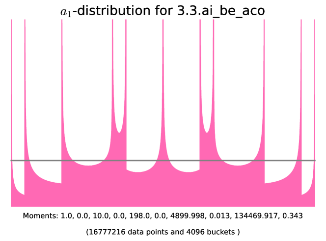
| (6.3-c) | 3.5.ai_bi_ado | |||
| (6.3-d) | 3.2.ad_h_al |
Proof.
Recall that over .
(6.3-a) If is geometrically isogenous to , then is
geometrically isogenous to . By Lemma 3.1.4
, where is the splitting degree of
, and so . By [14, Theorem 6],
we have that .
(6.3-b) In this case, by Lemma 3.1.4,
, where is the splitting
degree of and . As in the previous case,
.
(6.3-c) In this case over the base field.
Lemma 3.1.1 implies .
Example 6.3.2 (Non-simple ordinary threefolds of splitting type (6.3-a)).


6.4. Simple almost ordinary threefolds
Let be a simple and almost ordinary abelian threefold over . Recall that is in fact absolutely simple, so that the Frobenius polynomial is irreducible for every positive integer .
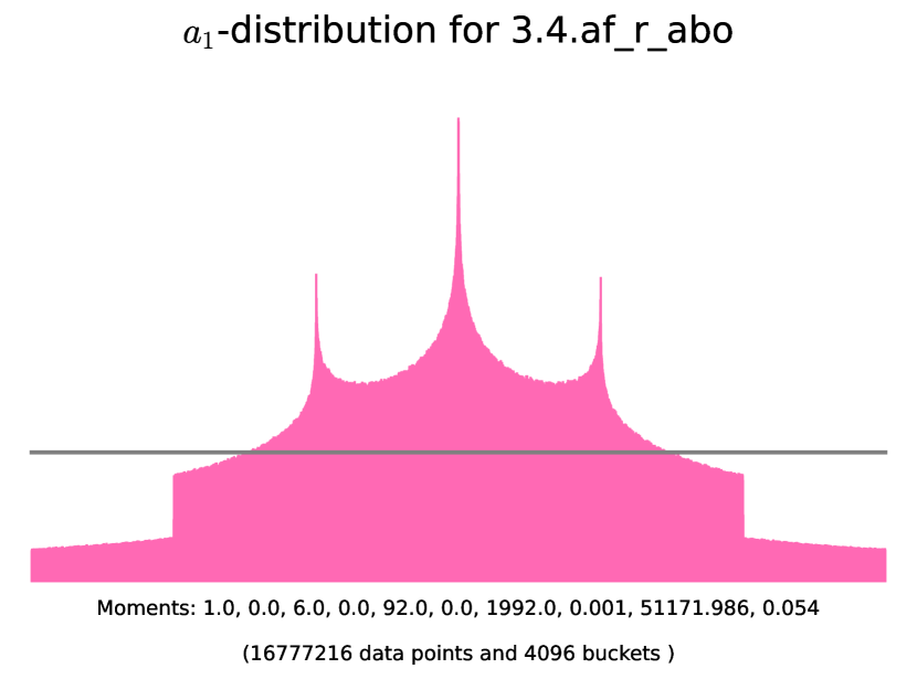
Lemma 6.4.1 (Node X-D in Figure 7).
Let be a simple almost ordinary abelian threefold over . The Serre–Frobenius group of can be read from Table 11.
| Def. 3.3.1 | class | Generator | Example | ||
| Neat | - | 1 | 3.2.ab_ab_c | ||
| Not neat | Yes | 1, 2, 3, 4, 6 | Example 6.4.2 | ||
| Not neat | No | 4, 6, 8, 12 | Example 6.4.2 |
Proof.
Let be the torsion order of , and consider the base extension . By [16, Theorem 5.7], we know that . Furthermore, since is absolutely simple, by the discussion in Section 6.1, the roots of are distinct and non-supersingular. If is neat, Remark (3.3.2.b) implies that . Assume then that is not neat, so that . Let be a Frobenius eigenvalue of . By [40, Theorem 1.1] and the discussion thereafter, we have that the sextic CM-field contains an imaginary quadratic field , and . Further, . Since has no torsion, this implies that . Moreover, this means that for some primitive555The primitivity of follows from the fact that is the minimal positive integer such that is torsion free. -th root of unity . Therefore,
| (15) |
If is odd, is also primitive, so that and . If is even, then we may distinguish between two cases. If , we know that so that in fact and implies that . If , then is a primitive -root of unity and .
In the setting where is not neat and , we notice that implies that , so the cases don’t occur when . Similarly, if , then . Thus, the torsion orders do not occur in this case. ∎
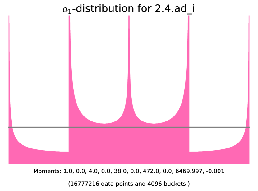
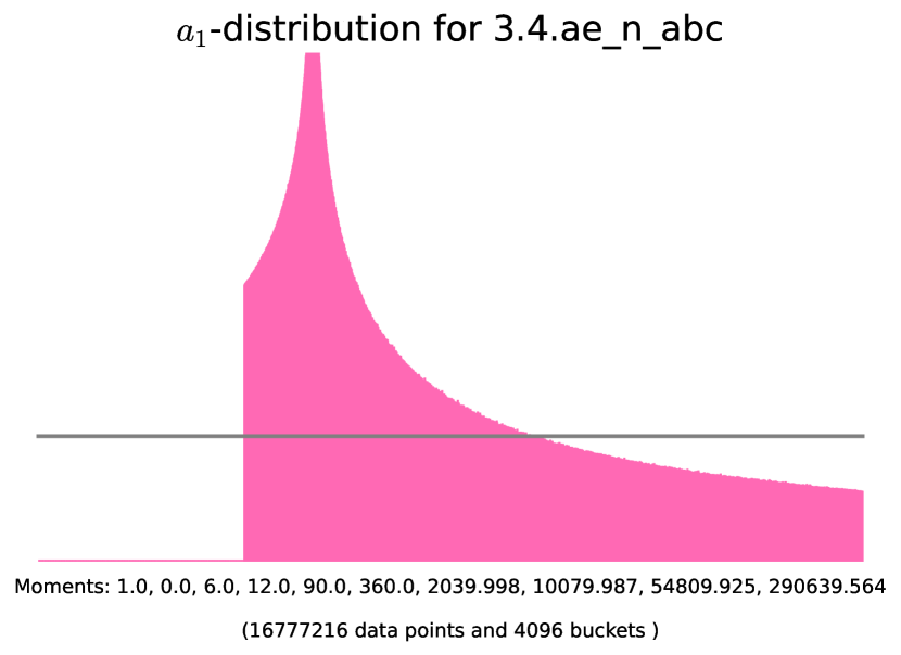
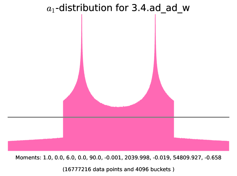
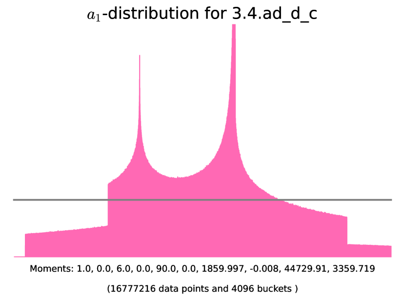
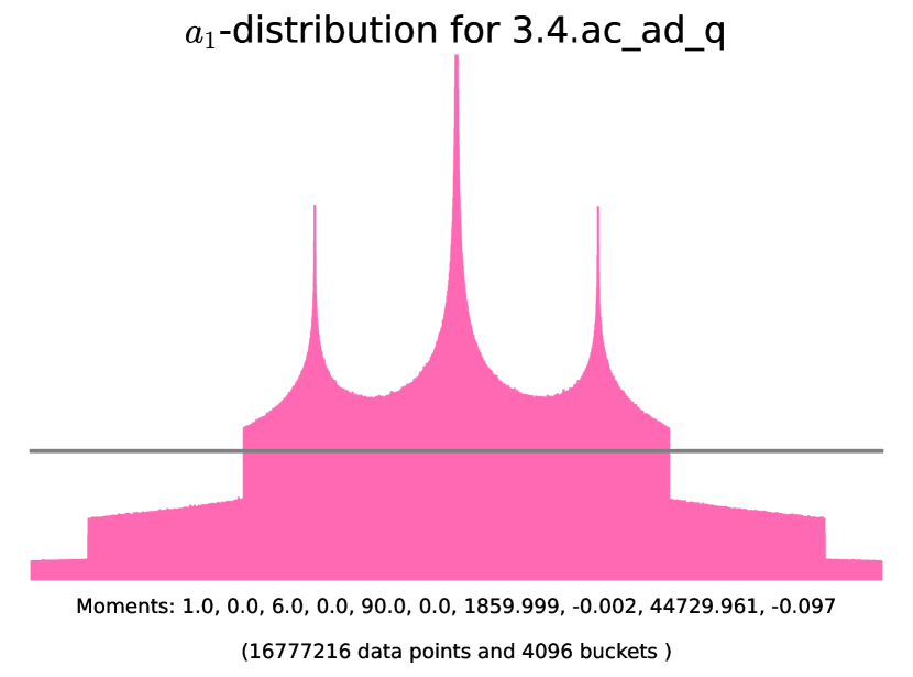
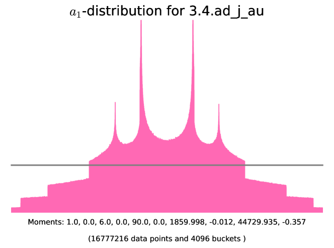
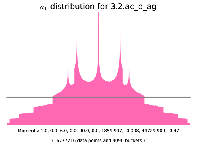
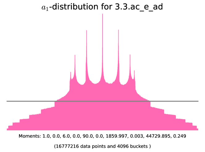
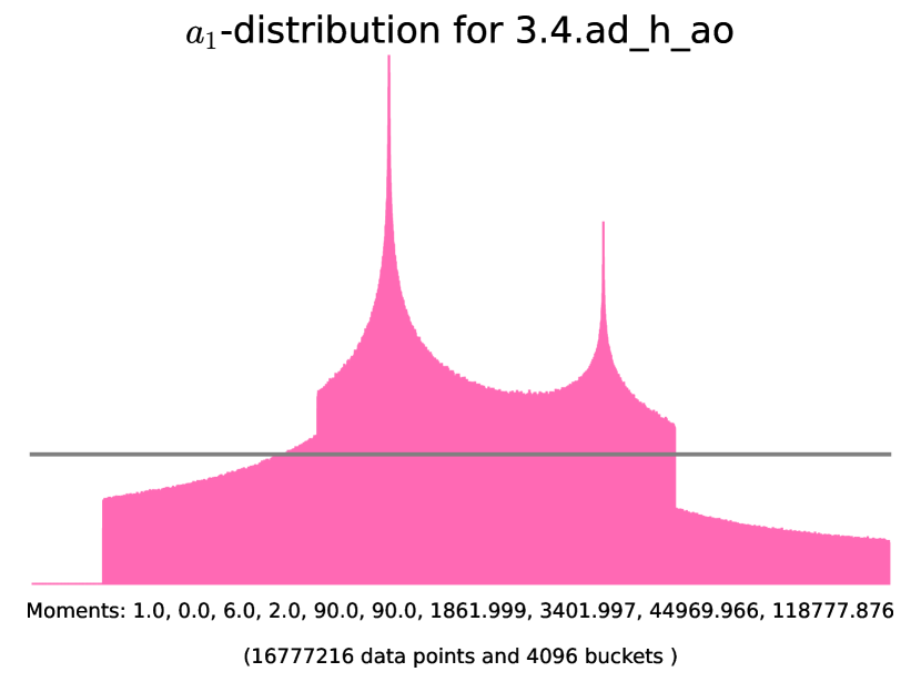
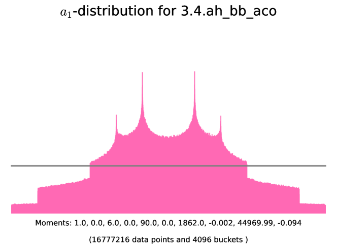
Example 6.4.2 (-distributions of simple almost ordinary abelian threefolds with angle rank ).
The histograms corresponding to the following examples are presented in Figure 11. In these examples we use SageMath [25] to initialize the degree-6 number field corresponding to the Frobenius polynomial, find the corresponding quadratic subfield , and check that is the root of unity in question. The code for generating the histograms is available on the GitHub repository [2].
6.5. Non-simple almost ordinary threefolds
Since is not simple, we have that for some surface and some elliptic curve . For this section, we let and be the Frobenius eigenvalues of and respectively. The normalized eigenvalues will be denoted by and . If has a geometric supersingular factor, by Honda–Tate theory, it must have a supersingular factor over the base field; and without loss of generality we may assume that this factor is .
Lemma 6.5.1 (Node X-E in Figure 7).
Proof.
First, suppose that has no supersingular factor. Thus is ordinary and is almost ordinary and absolutely simple. This implies that and are CM-fields of degrees and respectively, for every positive integer . In particular, for every . Let and consider the base extension . Since is not simple, [40, Theorem 1.1] implies that is neat. The eigenvalues of are all distinct and not supersingular, so that by Remark (3.3.2.b). The case where has a supersingular factor follows from Lemma 3.1.3. ∎
| class | Generator | Example | |||
| - | 3.3.ac_d_ae | ||||
| - | Figure 13 | ||||
| even | Figure 14 | ||||
| odd | Figure 14 |
6.6. Abelian threefolds of K3-type
In this section will be an abelian threefold defined over of -rank . The -Newton polygon of such a variety has slopes . This is the three-dimensional instance of abelian varieties of K3 type, which were studied by Zarhin in [38] and [37].
Definition 6.6.1.
An abelian variety defined over is said to be of K3-type if the set of Newton slopes is either or , and the segments of slope and have length one.
By [37, Theorem 5.9], simple abelian varieties of K3-type have maximal angle rank. As a corollary, we have another piece of the classification.
Lemma 6.6.2 (Node X-F in Figure 7).
Let be a simple abelian threefold over of -rank . Then has maximal angle rank and .
There are several examples of such , one of them being 3.2.ab_a_a. Now assume that is not simple, so that for some surface and elliptic curve .
Lemma 6.6.3 (Node X-G in Figure 7).
Let be a non-simple abelian threefold over of -rank . The Serre–Frobenius group of is given by Table 13.
We consider three cases:
-
(6.6.3-a)
is simple and almost ordinary, and is supersingular.
-
(6.6.3-b)
is non-simple and almost ordinary, and is supersingular.
-
(6.6.3-c)
is supersingular and is ordinary.
Proof.
As in Section 6.3, we let and be the Frobenius eigenvalues of and respectively. Denote the normalized eigenvalues by and .
Suppose first that is of type (6.6.3-a). By Lemma 5.3.1, the set is multiplicatively independent. Since is a root of unity, for the set of possible torsion orders for supersingular elliptic curves. Thus in this case, and is generated by .
If is of type (6.6.3-b), then with ordinary and supersingular. By Lemma 3.1.3, , with in the set of possible torsion orders of non-simple supersingular surfaces.
If is of type (6.6.3-c), we have for in the set of possible torsion orders of supersingular surfaces from Lemma 5.5.1 and Lemma 5.6.1. ∎
| Splitting type | class | Generator | Example | |
| Absolutely simple | 3.2.ab_a_a | |||
| (6.6.3-a) | - | |||
| (6.6.3-b) | in Table 8 | - | ||
| (6.6.3-c) | Figure 16 |
The following examples are all of splitting type (6.6.3-c), since this splitting type contains all the new Serre–Frobenius groups appearing in Table 13. The histograms corresponding to these examples are presented in Figure 16.


6.7. Absolutely simple p-rank 0 threefolds
In this section, will be a non-supersingular -rank abelian threefold over . Since the -Newton polygon of the Frobenius polynomial has slopes and , each with multiplicity three, it follows that is absolutely simple, since the slope does not occur for abelian varieties of smaller dimension. Let denote the dimension of over its center. We consider two cases:
-
(6.7-a)
There exists such that . In this case we have and is as in Theorem 6.1.1, so that divides .
-
(6.7-b)
for every positive integer .
Lemma 6.7.1 (Node X-H in Figure 7).
| Case | class | Generator | ||
| (6.7-a) | ||||
| (6.7-b) | - |
Remark 6.7.2.
The techniques for proving the Generalized Lenstra–Zarhin result in [8, Theorem 1.5], cannot be applied to this case. Thus, even the angle rank analysis in this case is particularly interesting.
Proof.
Suppose first that is of type (6.7-a), and let be the minimal positive integer such that . Maintaining previous notation, implies that and for -th roots of unity and , whose orders have lcm . By Lemma 2.3.2, this implies that . We conclude that and . To calculate the set of possible torsion orders, assume that . Then is a quadratic imaginary subextension of , and we can argue as in the proof of Theorem 3.2.1 (with ) to conclude that .
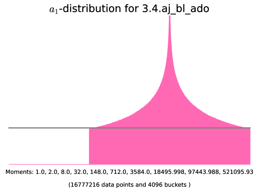
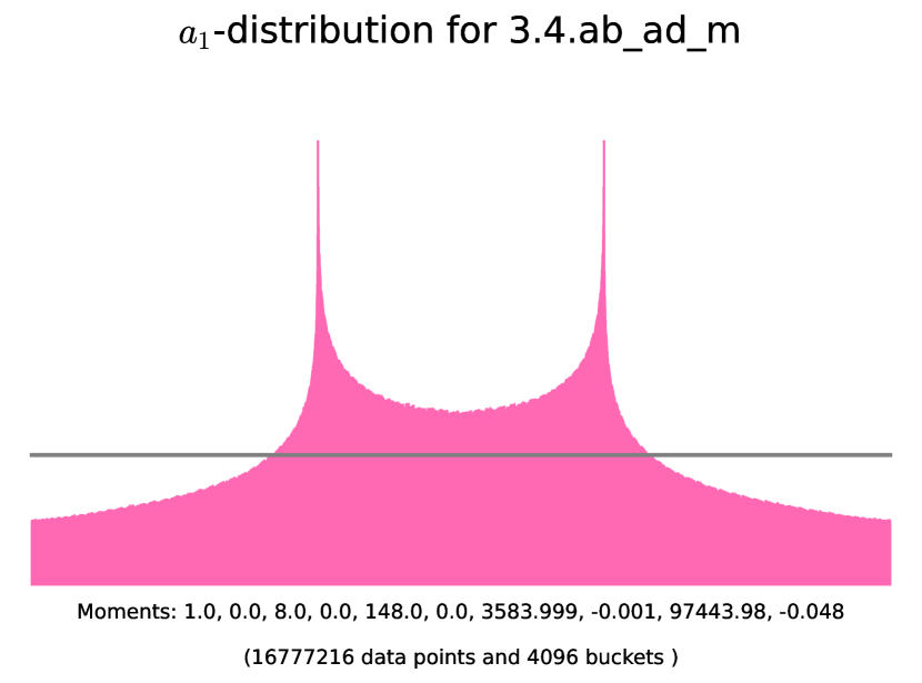
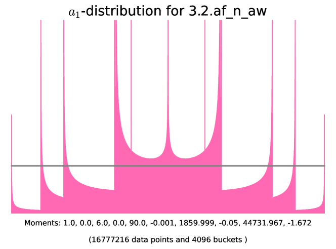
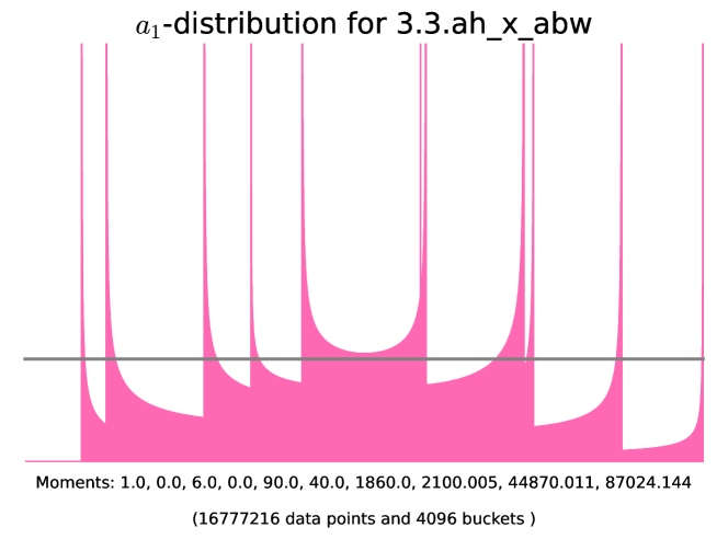
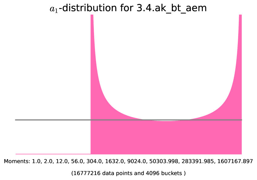
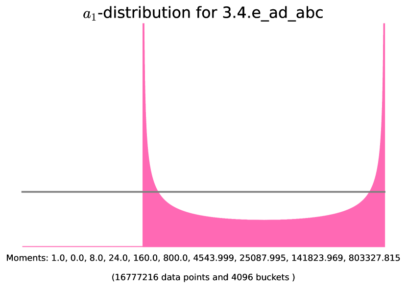
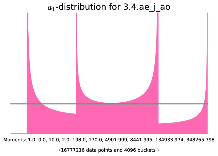
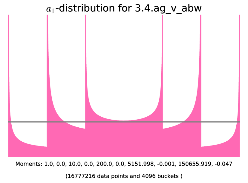
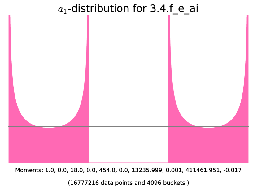
Example 6.7.3 (-distribution for -rank 0 non-supersingular threefolds of splitting type (6.7-a)).
The histograms corresponding to these examples are presented in Figure 17. Note that the first one already showed up in Figure 9, while the other ones appeared in Figure 8.
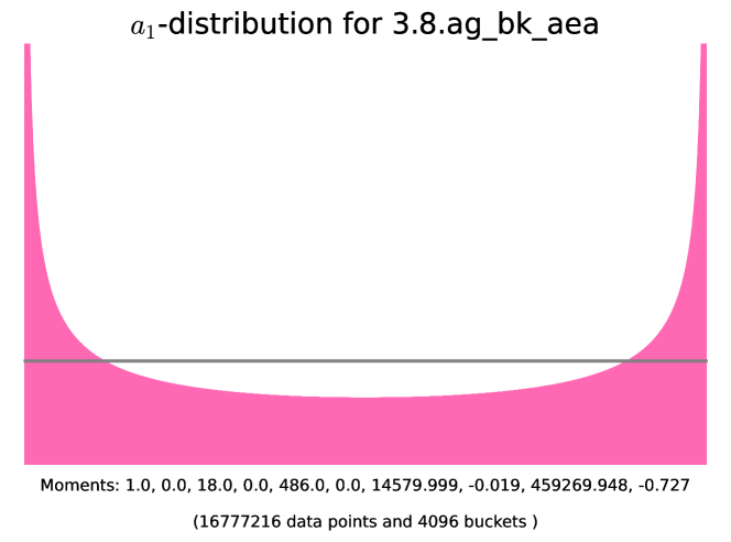
-
(A)
() The isogeny class 3.8.ag_bk_aea satisfies . Note that divides .
-
(B)
() The isogeny class 3.2.a_a_ac has angle rank and irreducible Frobenius polynomial . The cubic base extension gives the isogeny class 3.8.ag_bk_aea with reducible Frobenius polynomial . Note that divides .
-
(C)
() The isogeny class 3.8.ai_bk_aeq has angle rank and irreducible Frobenius polynomial . Its base change over a degree extension is the isogeny class 3.2097152.ahka_bfyoxc_adesazpwa with Frobenius polynomial
In this example, , so that divides .


6.8. Simple supersingular threefolds
Nart and Ritzenthaler [21] showed that the only degree supersingular -Weil numbers are the conjugates of
Building on their work, Haloui [12, Proposition 1.5] completed the classification of simple supersingular threefolds. This classification is also discussed in [29]; and we adapt their notation for the polynomials of Z-3 type. Denoting by the isogeny class of abelian threefolds over with Frobenius polynomial , the following lemma gives the classification of Serre–Frobenius groups of simple supersingular threefolds, which is a corollary of Haloui’s result.
Lemma 6.8.1 (Node X-I in Figure 7).
Let be a simple supersingular abelian threefold defined over . The Serre–Frobenius group of is classified according to Table 15.
| Type | Example | |||||
| even | Z-1 | 3.9.d_j_bb | ||||
| even | Z-1 | 3.9.ad_j_abb | ||||
| even | Z-1 | 3.4.a_a_i | ||||
| even | Z-1 | 3.4.a_a_ai | ||||
| odd | Z-3 | 3.7.h_v_bx | ||||
| odd | Z-3 | 3.7.ah_v_abx | ||||
| odd | Z-3 | 3.3.a_a_j | ||||
| odd | Z-3 | 3.3.a_a_aj |
Proof.
By Theorem 6.1.1 and the discussion following it, we know that the Frobenius polynomial of every supersingular threefold , coincides with the minimal polynomial with in some row of the table. The first four rows of Table 15 correspond to isogeny classes of type (Z-1). By the discussion in Section 3.4, the minimal polynomials are of the form666Recall that . and the normalized polynomials are just the usual cyclotomic polynomials .
The last four rows of Table 15 correspond to isogeny classes of type (Z-3). The normalized Frobenius polynomials are , and Noting that and we conclude that the unit groups are generated by and respectively. ∎
6.9. Non-simple supersingular threefolds
If is a non-simple supersingular abelian threefold over , then there are two cases:
-
(6.9.0-a)
, with a simple supersingular surface over and a supersingular elliptic curve.
-
(6.9.0-b)
, where each is a supersingular elliptic curve.
The classification of the Serre–Frobenius group in these cases can be summarized in the following lemma.
Lemma 6.9.1 (Node X-J in Figure 7).
If is a non-simple supersingular abelian threefold as in Case (6.9.0-a), then , for , where
-
•
if is even, , and
-
•
if is odd, .
Proof.
Lemma 6.9.2 (Node X-J in Figure 7).
If is a non-simple supersingular abelian threefold as in Case (6.9.0-b), then , for , where
-
•
if is even, , and
-
•
if is odd, .
Proof.
We know that is the degree of the extension over which all the elliptic curve factors become isogenous. This is precisely the least common multiple of the ’s. From Table 3, we can calculate the various possibilities for the ’s depending on the parity of . ∎
6.10. Acknowledgements
We would like to thank David Zureick-Brown, Kiran Kedlaya, Francesc Fité, Brandon Alberts, Edgar Costa, and Andrew Sutherland for useful conversations about this paper. We thank Yuri Zarhin for providing us with useful references, and Hendrik Lenstra for pointing out one of the missing cases in Section 4. We would also like to thank Everett Howe for helping us with a missing piece of the puzzle in Theorem 3.2.1. This project started as part of the Rethinking Number Theory workshop in 2021. We thank the organizers of the workshop for giving us the opportunity and space to collaborate, and the funding sources for the workshop: AIM, the Number Theory Foundation, and the University of Wisconsin-Eau Claire Department of Mathematics. We are also grateful to Rachel Pries for her guidance at the beginning of the workshop, which helped launch this project. Finally, we thank the anonymous referee for the elucidating and pertinent suggestions that improved the exposition and results in the paper.
References
- Ahmadi and Shparlinski [2010] Ahmadi, O. and I. E. Shparlinski (2010). On the distribution of the number of points on algebraic curves in extensions of finite fields. Math. Res. Lett. 17(4), 689–699.
- [2] Arango-Piñeros, S., D. Bhamidipati, and S. Sankar. Code accompanying “Frobenius distributions of abelian varieties over finite fields”. https://github.com/sarangop1728/Frobenius-distributions-AVs-Fq.
- Chai et al. [2014] Chai, C.-L., B. Conrad, and F. Oort (2014). Complex multiplication and lifting problems, Volume 195 of Mathematical Surveys and Monographs. American Mathematical Society, Providence, RI.
- Chi [1992] Chi, W. C. (1992). -adic and -adic representations associated to abelian varieties defined over number fields. Amer. J. Math. 114(2), 315–353.
- Deuring [1941] Deuring, M. (1941). Die Typen der Multiplikatorenringe elliptischer Funktionenkörper. Volume 14, pp. 197–272.
- Diem and Naumann [2003] Diem, C. and N. Naumann (2003). On the structure of Weil restrictions of abelian varieties. J. Ramanujan Math. Soc. 18(2), 153–174.
- Dupuy et al. [2021] Dupuy, T., K. Kedlaya, D. Roe, and C. Vincent ([2021] ©2021). Isogeny classes of abelian varieties over finite fields in the LMFDB. In Arithmetic geometry, number theory, and computation, Simons Symp., pp. 375–448. Springer, Cham.
- Dupuy et al. [2024] Dupuy, T., K. S. Kedlaya, and D. Zureick-Brown (2024). Angle ranks of abelian varieties. Math. Ann. 389, 169–185.
- Fité [2015] Fité, F. (2015). Equidistribution, -functions, and Sato-Tate groups. In Trends in number theory, Volume 649 of Contemp. Math., pp. 63–88. Amer. Math. Soc., Providence, RI.
- Fité et al. [2012] Fité, F., K. S. Kedlaya, V. Rotger, and A. V. Sutherland (2012). Sato-Tate distributions and Galois endomorphism modules in genus 2. Compos. Math. 148(5), 1390–1442.
- Fité et al. [2023] Fité, F., K. S. Kedlaya, and A. V. Sutherland (2023). Sato-Tate groups of abelian threefolds.
- Haloui [2010] Haloui, S. (2010). The characteristic polynomials of abelian varieties of dimensions 3 over finite fields. J. Number Theory 130(12), 2745–2752.
- Honda [1968] Honda, T. (1968). Isogeny classes of abelian varieties over finite fields. J. Math. Soc. Japan 20, 83–95.
- Howe and Zhu [2002] Howe, E. W. and H. J. Zhu (2002). On the existence of absolutely simple abelian varieties of a given dimension over an arbitrary field. J. Number Theory 92(1), 139–163.
- Krajíček and Scanlon [2000] Krajíček, J. and T. Scanlon (2000). Combinatorics with definable sets: Euler characteristics and Grothendieck rings. Bull. Symbolic Logic 6(3), 311–330.
- Lenstra and Zarhin [1993] Lenstra, Jr., H. W. and Y. G. Zarhin (1993). The Tate conjecture for almost ordinary abelian varieties over finite fields. In Advances in number theory (Kingston, ON, 1991), Oxford Sci. Publ., pp. 179–194. Oxford Univ. Press, New York.
- LMFDB Collaboration [2024] LMFDB Collaboration, T. (2024). The L-functions and modular forms database. https://www.lmfdb.org. [Online; accessed 15 March 2024].
- Maisner and Nart [2002] Maisner, D. and E. Nart (2002). Abelian surfaces over finite fields as Jacobians. Experiment. Math. 11(3), 321–337. With an appendix by Everett W. Howe.
- Milne [2017] Milne, J. S. (2017). Algebraic groups, Volume 170 of Cambridge Studies in Advanced Mathematics. Cambridge University Press, Cambridge. The theory of group schemes of finite type over a field.
- Morris [1977] Morris, S. A. (1977). Pontryagin duality and the structure of locally compact abelian groups. London Mathematical Society Lecture Note Series, No. 29. Cambridge University Press, Cambridge-New York-Melbourne.
- Nart and Ritzenthaler [2008] Nart, E. and C. Ritzenthaler (2008). Jacobians in isogeny classes of supersingular abelian threefolds in characteristic 2. Finite Fields Appl. 14(3), 676–702.
- Oort [2008] Oort, F. (2008). Abelian varieties over finite fields. In Higher-dimensional geometry over finite fields, Volume 16 of NATO Sci. Peace Secur. Ser. D Inf. Commun. Secur., pp. 123–188. IOS, Amsterdam.
- Pontrjagin [1934] Pontrjagin, L. (1934). The theory of topological commutative groups. Ann. of Math. (2) 35(2), 361–388.
- Rűck [1990] Rűck, H.-G. (1990). Abelian surfaces and Jacobian varieties over finite fields. Compositio Math. 76(3), 351–366.
- Sage Developers [2024] Sage Developers, T. (2024). Sagemath, the Sage Mathematics Software System (Version 9.5). https://www.sagemath.org.
- Serre [1998] Serre, J.-P. (1998). Abelian -adic representations and elliptic curves, Volume 7 of Research Notes in Mathematics. A K Peters, Ltd., Wellesley, MA. With the collaboration of Willem Kuyk and John Labute, Revised reprint of the 1968 original.
- Serre [2013] Serre, J.-P. (2013). Oeuvres/Collected papers. IV. 1985–1998. Springer Collected Works in Mathematics. Springer, Heidelberg. Reprint of the 2000 edition [MR1730973].
- Serre [2020] Serre, J.-P. ([2020] ©2020). Rational points on curves over finite fields, Volume 18 of Documents Mathématiques (Paris) [Mathematical Documents (Paris)]. Société Mathématique de France, Paris. With contributions by Everett Howe, Joseph Oesterlé and Christophe Ritzenthaler.
- Singh et al. [2014] Singh, V., G. McGuire, and A. Zaytsev (2014). Classification of characteristic polynomials of simple supersingular abelian varieties over finite fields. Funct. Approx. Comment. Math. 51(2), 415–436.
- Sutherland [2019] Sutherland, A. V. ([2019] ©2019). Sato-Tate distributions. In Analytic methods in arithmetic geometry, Volume 740 of Contemp. Math., pp. 197–248. Amer. Math. Soc., [Providence], RI.
- Tate [1966] Tate, J. (1966). Endomorphisms of abelian varieties over finite fields. Invent. Math. 2, 134–144.
- Tate [1971] Tate, J. (1971). Classes d’isogénie des variétés abéliennes sur un corps fini (d’après T. Honda). In Séminaire Bourbaki. Vol. 1968/69: Exposés 347–363, Volume 175 of Lecture Notes in Math., pp. Exp. No. 352, 95–110. Springer, Berlin.
- Waterhouse [1969] Waterhouse, W. C. (1969). Abelian varieties over finite fields. Ann. Sci. École Norm. Sup. (4) 2, 521–560.
- Weil [1949] Weil, A. (1949). Numbers of solutions of equations in finite fields. Bull. Amer. Math. Soc. 55, 497–508.
- Xing [1994] Xing, C. (1994). The characteristic polynomials of abelian varieties of dimensions three and four over finite fields. Sci. China Ser. A 37(2), 147–150.
- Xing [1996] Xing, C. (1996). On supersingular abelian varieties of dimension two over finite fields. Finite Fields Appl. 2(4), 407–421.
- Zarhin [1991] Zarhin, Y. G. (1991). Abelian varieties of type and -adic representations. In Algebraic geometry and analytic geometry (Tokyo, 1990), ICM-90 Satell. Conf. Proc., pp. 231–255. Springer, Tokyo.
- Zarhin [1993] Zarhin, Y. G. (1993). Abelian varieties of type. In Séminaire de Théorie des Nombres, Paris, 1990–91, Volume 108 of Progr. Math., pp. 263–279. Birkhäuser Boston, Boston, MA.
- Zarhin [1994] Zarhin, Y. G. (1994). The Tate conjecture for nonsimple abelian varieties over finite fields. In Algebra and number theory (Essen, 1992), pp. 267–296. de Gruyter, Berlin.
- Zarhin [2015] Zarhin, Y. G. (2015). Eigenvalues of Frobenius endomorphisms of abelian varieties of low dimension. J. Pure Appl. Algebra 219(6), 2076–2098.
- Zhu [2001] Zhu, H. J. (2001). Supersingular abelian varieties over finite fields. J. Number Theory 86(1), 61–77.
- Zywina [2022] Zywina, D. (2022). Determining monodromy groups of abelian varieties. Res. Number Theory 8(4), Paper No. 89, 53.